Association of oxygen vacancies with impurity metal ions in lead titanate

Abstract

Thermodynamic, structural and electronic properties of isolated copper and iron atoms as well as their complexes with oxygen vacancies in tetragonal lead titanate are investigated by means of first principles calculations. Both dopants exhibit a strong chemical driving force for the formation of $M_{\text{Ti}}-V_{\text{O}}$ ($M$ = Cu, Fe) defect associates. The most stable configurations corresponds to a local dipole aligned along the tetragonal axis parallel to the spontaneous polarization. Local spin moments are obtained and the calculated spin densities are discussed. The calculations provide a simple and consistent explanation for the experimental findings. The results are discussed in the context of models for degradation of ferroelectric materials.

I Introduction

Piezoelectric materials transform electric signals into mechanical response and vice versa. They are widely used in sensors and actuators as well as in non-volatile memory devices. The properties of piezoelectrics and their behavior in the presence of electric fields are intimately linked to the defect structures (point defects, domain walls, grain boundaries) present in these materials.

Defect dipoles, for instance, formed by the association of oxygen vacancies with metal impurities affect the switching behavior as well as aging and fatigue of piezoelectric materials. Warren et al. (1995a) Their existence has been shown both experimentally Warren et al. (1995b, a); Meštrić et al. (2004); Meštrić et al. (2005) and theoretically. Pöykkö and Chadi (1999) However, a comprehensive microscopic picture of the electronic, structural and kinetic properties of these defect associates is still lacking. Such detailed knowledge is, however, a prerequisite for understanding electrical “aging” and ferroelectric “fatigue” as exemplified by the model by Arlt and Neumann,Neumann and Arlt (1987); Arlt and Neumann (1988) which relates these macroscopic degradation phenomena to microscopic processes. Since the time the first phenomenological models were developed Neumann and Arlt (1987); Arlt and Neumann (1988) quantum mechanical methods have become available which are both efficient and sufficiently reliable for assessing the energetics of point defect and associates, directly. In the past, several studies addressed the properties of intrinsic point defects with particular attention to oxygen vacancies. Park and Chadi (1998); Pöykkö and Chadi (2000a); Cockayne and Burton (2004); Park (2003); He and Vanderbilt (2003); Zhang et al. (2006) The role of dopants and impurities and the formation of defect dipoles has also been elucidated Pöykkö and Chadi (1999, 2000b); Meštrić et al. (2004); Meštrić et al. (2005) but important aspects such as the dependence of the formation energies on the Fermi level and the charge state have not been investigated in sufficient detail. Also, a comparative study of the different possible metal impurity-oxygen vacancy configurations, which could serve as input for the defect models referenced above, is not available yet. Such information is, however, crucial both for understanding the generic properties of different impurities/dopants and for identifying properties which differentiate them, in particular with regard to their effect on aging and fatigue. These considerations motivate the present work, in which density functional theory calculations are employed to study the energy surface for unbound oxygen vacancies and oxygen vacancies complexed with Fe or Cu impurities in tetragonal lead titanate. The results are discussed in the context of existing defect models and have been used to interpret recent electron spin resonance experiments.EicErhTra07

II Methodology

II.1 Computational details

Quantum mechanical calculations based on density functional theory (DFT) were carried out using the Vienna ab-initio simulation package (vasp) which implements the pseudopotential-plane wave approach. Kresse and Hafner (1993, 1994); Kresse and Furthmüller (1996a, b) The projector-augmented wave method was employed for representing the ionic cores and core electrons. Blöchl (1994); Kresse and Joubert (1999) In accord with earlier calculations (see e.g., Refs. Park and Chadi, 1998 and Meštrić et al., 2005) the $5d$ electrons of Pb and the $3s$ and $3p$ electrons of Ti were treated as semi-core states, while for Cu and Fe the valence configuration included the $4d$, $3d$ and $3p$ electrons. All calculations were performed using Gaussian smearing with a width of $\sigma=0.2\,\text{eV}$ and a $4\times 4\times 4$ Monkhorst-Pack mesh for Brillouin zone sampling. Monkhorst and Pack (1976) Calculations were carried out using the local spin density approximation (LSDA) to account for the magnetic behavior of iron.Note1 Some calculations were also repeated using the non-spin polarized local density approximation (LDA). The difference between the LDA and LSDA results allows to estimate the spin contribution for a particular defect or charge state.

With this computational setup, we obtain a lattice constant of $a_{0}=3.866\,\text{\AA}$ and an axial ratio of $c/a=1.05$ for the tetragonal phase of PbTiO₃ in reasonable agreement with experiment. The calculated band gap of 1.47 eV is considerably smaller than the experimental value but consistent with the well known LSDA band gap error. Since there is no unique procedure for correcting the band gap error (see e.g, Refs. Persson et al., 2005; Janotti and Van de Walle, 2006; Erhart and Albe, ), in the present work, we abstain from any explicit corrections and discuss the electronic transition levels relative to the calculated band edges instead (see also our discussion in Sec. III.1).

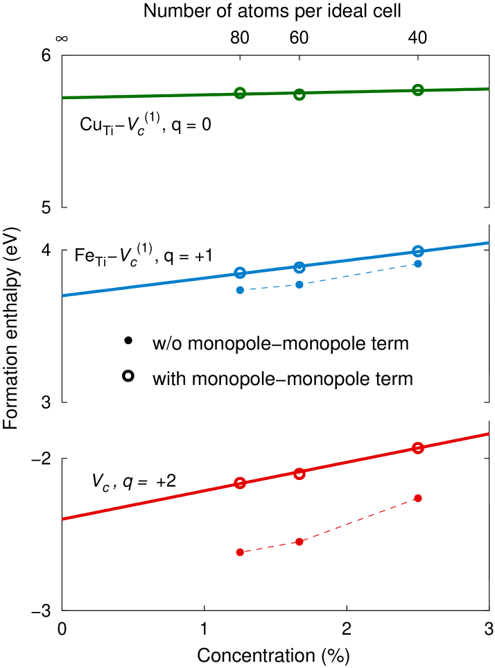
Figure 1: (Color online) Finite-size scaling of formation enthalpies to obtain formation energies in the limit of infinite dilution for three of the most important defects. The small filled and large open circles show the data before and after application of the monopole-monopole correction term.

In order to model the defect configurations, super cells containing $2\times 2\times 2$ to $2\times 2\times 4$ unit cells equivalent to 40 to 80 atoms were employed. Each configuration was relaxed until the maximum force was less than 15 meV/Å. For charged defects a homogeneous background charge was added. Finite-size scaling was employed in order to obtain the formation and binding energies at infinite dilution. Lento et al. (2002); Erhart et al. (2006) For the charged defect calculations monopole-monopole interactions were explicitly corrected Makov and Payne (1995); Lento et al. (2002) using values of $\epsilon_{11}^{S}=100$ and $\epsilon_{33}^{S}=34$ for the static dielectric tensor, Note2 while higher order terms were implicitly included by the finite-size scaling procedure. Lento et al. (2002); Erhart et al. (2006) Both the effect of the monopole-monopole term and the finite-size procedure are illustrated in Fig. 1 for three of the most important defects which demonstrates that the finite-size scaling approach works reliably in the present case. The extrapolation errors of the finite-size scaling procedure are given in Tables 1, 2, and 3. These values are a measure for the quality of the finite-size scaling procedure only, and do not include other errors intrinsic to DFT.

II.2 Formation energies

The formation energy of an intrinsic defect in charge state, $q$, depends on the relative chemical potentials of the constituents, $\Delta\mu_{i}$, and the Fermi level (electron chemical potential), $\mu_{e}$, according to Qian et al. (1988); Zhang and Northrup (1991)

$$\Delta E_{D}^{f} =(E_{D}-E_{H})+q(E_{\text{VBM}}+\mu_{e})$$

$$\quad-\sum_{i}\Delta n_{i}(\mu_{i}^{bulk}+\Delta\mu_{i})$$ (1)

where $E_{D}$ is the total energy of the defective system, $E_{H}$ is the total energy of the perfect reference cell, $E_{\text{VBM}}$ is the position of the valence band maximum, $\Delta n_{i}$ denotes the difference between the number of atoms of type $i$ in the reference cell with respect to the defective cell, and $\mu_{i}^{bulk}$ is the chemical potential of the reference phase of atom type $i$. In the present context we are not concerned with the effect of the chemical environment ($\Delta\mu_{i}$ in equation (1)) but focus on the transition levels and the binding energies between oxygen vacancies and metal impurities/dopants (see equation (2) below), both of which are independent of the chemical potentials.

The binding energy for the metal impurity-oxygen vacancy ($M_{\text{Ti}}-V_{\text{O}}$) associates considered below is calculated as the difference between the formation energies of the defect complex and the isolated defects

$$E_{b} =\Delta E_{D}^{f}[M_{\text{Ti}}-V_{\text{O}}]-\Delta E_{D}^{f}[M_{\text{Ti}}]-\Delta E_{D}^{f}[V_{\text{O}}].$$ (2)

The binding energy depends on the Fermi level due to the Fermi level dependence of the formation energies. For a given value of $\mu_{e}$ the difference in equation (2) is calculated between the most stable charge states for each defect involved. By insertion of equation (1) into (2) one can show that the terms with $\Delta n_{i}$ cancel, whence $E_{b}$ is independent of the chemical potentials, $\Delta\mu_{i}$. Following the sign convention introduced via equation (2), negative values for $E_{b}$ imply that the system gains energy by association, whereas positive values imply an effective repulsion between the isolated defects.

III Results

III.1 Isolated oxygen vacancies

Table 1: Formation energies (eV) for unbound oxygen vacancies in tetragonal lead titanate for a Fermi level at the valence band maximum ($\mu_{e}=0\,\text{eV}$) and metal-rich conditions ($\Delta\mu_{\text{Pb}}=\Delta\mu_{\text{Ti}}=0\,\text{eV}$). The finite-size scaling extrapolation errors are given in brackets in the last column.

Defect		$\boldsymbol{40}$	$\boldsymbol{60}$	$\boldsymbol{80}$	extrapolated
$V_{ab}$	$0$	$0.96$	$0.95$	$0.95$	$0.95$	$(<0.01)$
	$+1$	$-0.40$	$-0.43$	$-0.43$	$-0.47$	$(0.01)$
	$+2$	$-1.64$	$-1.62$	$-1.62$	$-1.60$	$(<0.01)$
$V_{c}$	$0$	$1.07$	$0.87$	$0.70$	$0.35$	$(0.08)$
	$+1$	$-0.59$	$-0.88$	$-0.96$	$-1.35$	$(0.06)$
	$+2$	$-1.93$	$-2.10$	$-2.16$	$-2.40$	$(0.03)$

The crystallographic structure of a tetragonal perovskite possesses two symmetrically inequivalent oxygen sites which are located within the $ab$-plane and along the $c$-axis, respectively. Based on DFT calculations, Park and Chadi Park and Chadi (1998) identified one possible vacancy configuration along the $c$-axis ($V_{c}$) and two distinct vacancies configurations within the $ab$-plane ($V_{ab}^{sw}$, $V_{ab}^{ud}$). The latter two configurations differ in the orientation of the polarization above and below the vacancy plane. In the present work we have found the “up-down” configuration ($V_{ab}^{ud}$, see Ref. Park and Chadi, 1998 for nomenclature), in which the polarization vectors are oriented head-to-head in the vacancy plane, to be highly unstable with respect to the “switchable” configuration ($V_{ab}^{sw}$), which is characterized by a uniform orientation of the polarization vector. Although Park and Chadi did not provide a quantitative energy comparison for $V_{ab}^{sw}$ and $V_{ab}^{ud}$ due to missing data for the 180^∘-domain wall energy, they estimated the $V_{ab}^{sw}$ configuration to be lower in energy. Park and Chadi (1998) For these reasons, we focus on the $V_{ab}^{sw}$ configuration which for the sake of brevity in the following is denoted $V_{ab}$.

Table 1 summarizes the formation energies for unbound oxygen vacancies obtained for extreme metal-rich conditions ($\Delta\mu_{\text{Pb}}=\Delta\mu_{\text{Ti}}=0\,\text{eV}$). In all charge states the $c$-type vacancy is energetically preferred over the $ab$-type vacancy in agreement with the calculations in Ref. Park and Chadi, 1998. For infinite dilution (extrapolated values in Table 1 the energy difference is as large as 0.8 eV for $q=+2$ which is on the order of magnitude of the energy barrier for migration.Erhart et al.

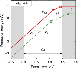
Figure 2: (Color online) Variation of the formation energy of unbound oxygen vacancies with the Fermi level for extreme metal-rich conditions ($\Delta\mu_{\text{Pb}}=\Delta\mu_{\text{Ti}}=0\,\text{eV}$). The white area corresponds to the calculated band gap. The numbers indicate the defect charge state.

The variation of the formation energy with the Fermi level is shown in Fig. 2. Practically over the entire band gap oxygen vacancies are doubly positively charged. For the given chemical conditions the formation energies are negative which indicates that the material is unstable for these chemical potentials ($\Delta\mu_{\text{Pb}}=\Delta\mu_{\text{Ti}}=0\,\text{eV}$). If the oxygen partial pressure is raised (i.e., $\Delta\mu_{\text{Ti}}$ and $\Delta\mu_{\text{Pb}}$ become less negative while $\Delta\mu_{\text{O}}$ becomes more negative), the oxygen vacancy formation energy increases and the stability condition is fulfilled.

On first sight the present finding is at variance with the calculations in Ref. Park, 2003 in which the +2/0 transition level of the oxygen vacancy is located in the middle of the band gap. This finding is, however, a consequence of the corrections applied in that work: In order to correct for the the band gap error the conduction band minimum was rigidly shifted upwards without correcting the formation energies. If this shift is omitted the results of Ref. Park, 2003 and the findings of the present work are consistent with each other. The approach in Ref. Park, 2003 ignores the fact that in the case of singly charged ($V_{\text{O}}^{\scriptscriptstyle{\bullet}}$) and neutral oxygen vacancies ($V_{\text{O}}^{\times}$) the excess electron(s) occupy conduction band states. In order to maintain internal consistency, a correction term Persson et al. (2005) on the order of $z_{e}\Delta E_{G}$ would have to be added to the formation energies of $V_{\text{O}}^{\scriptscriptstyle{\bullet}}$ and $V_{\text{O}}^{\times}$, where $z_{e}$ is the number of occupied conduction band states and $\Delta E_{G}$ denotes the difference between the calculated and the experimental band gap. Note3 If these energy terms are included, the +2/+1 (+2/0) transition is no longer located in the middle of the (experimental) band gap but near the conduction band minimum. This is equivalent to the location of the transition level with respect to the calculated CBM if no correction is applied.

III.1.1 Isolated copper impurities

Table 2: Formation energies (LSDA) in units of eV for isolated and complexed Cu-impurities on Ti-sites ($\text{Cu}_{\text{Ti}}$) in tetragonal lead titanate for a Fermi level at the valence band maximum ($\mu_{e}=0\,\text{eV}$) and metal-rich conditions ($\Delta\mu_{\text{Pb}}=\Delta\mu_{\text{Ti}}=\Delta\mu_{\text{Cu}}=0\,\text{eV}$). The finite-size scaling extrapolation errors are given in brackets in the last but one column. $\Delta n_{\upharpoonleft\downharpoonright}$ denotes the difference between the number of electrons in spin-up and spin-down states.

Defect		$\boldsymbol{\Delta n_{\upharpoonleft\downharpoonright}}$	$\boldsymbol{40}$	$\boldsymbol{60}$	$\boldsymbol{80}$	extrapolated
$\text{Cu}_{\text{Ti}}$
	$-3$	$-$	$11.81$	$12.04$	$12.06$	$12.35$	$(0.10)$
	$-2$	$1$	$10.16$	$10.28$	$10.30$	$10.46$	$(0.05)$
	$-1$	$2$	$9.74$	$9.79$	$9.81$	$9.88$	$(0.01)$
	$0$	$-$	$9.97$	$9.95$	$10.07$	$10.11$	$(0.14)$
$\text{Cu}_{\text{Ti}}-V_{ab}$
	$-2$	$-$	$9.22$	$9.32$	$9.32$	$9.45$	$(0.06)$
	$-1$	$0$	$7.23$	$7.36$	$7.41$	$7.60$	$(0.01)$
	$0$	$1$	$6.43$	$6.45$	$6.48$	$6.52$	$(0.02)$
	$+1$	$0$	$6.67$	$6.62$	$6.60$	$6.52$	$(0.01)$
$\text{Cu}_{\text{Ti}}-V_{c}^{(1)}$
	$-2$	$-$	$8.83$	$8.91$	$8.91$	$9.01$	$(0.04)$
	$-1$	$0$	$6.86$	$6.94$	$6.99$	$7.11$	$(0.01)$
	$0$	$1$	$5.77$	$5.74$	$5.75$	$5.72$	$(0.03)$
	$+1$	$0$	$6.02$	$5.94$	$5.91$	$5.80$	$(0.01)$
$\text{Cu}_{\text{Ti}}-V_{c}^{(2)}$
	$-2$	$-$	$9.33$	$9.57$	$9.69$	$10.04$	$(<0.01)$
	$-1$	$0$	$7.29$	$7.59$	$7.77$	$8.24$	$(0.03)$
	$0$	$1$	$6.22$	$6.43$	$6.59$	$6.93$	$(0.06)$
	$+1$	$-$	$6.44$	$6.64$	$6.80$	$7.14$	$(0.07)$
$\text{Cu}_{\text{Ti}}-V_{c}^{(3)}$
	$-2$	$-$		$10.00$	$10.01$	$10.04$
	$-1$	$0$		$7.98$	$8.04$	$8.22$
	$0$	$1$		$6.76$	$6.75$	$6.74$
	$+1$	$-$		$6.97$	$6.89$	$6.68$
$\text{Cu}_{\text{Ti}}-V_{c}^{(4)}$
	$-2$	$-$			$10.21$
	$-1$	$0$			$8.26$
	$0$	$1$			$6.98$
	$+1$	$-$			$7.14$

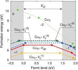
Figure 3: (Color online) Fermi level dependence of formation energies of free and complexed Cu impurities. Parallel lines imply equal charge states as indicated in the plot. The white stripe indicates the (calculated) band gap while the gray stripes indicate the valence and conduction bands, respectively. Extrapolated formation energies from Table 2 were used except for $\text{Cu}_{\text{Ti}}-V_{c}^{(4)}$ for which the data obtained with 80-atom cells are shown.

Since there is experimental evidence that copper impurities in lead titanate preferentially occupy Ti-sites Eichel et al. (2004, 2005a, 2005b) only the substitutional position was considered ($\text{Cu}_{\text{Ti}}$) in the present calculations. The calculated formation energies for different charge states of $\text{Cu}_{\text{Ti}}$ are compiled in Table 2 for extreme metal-rich conditions ($\Delta\mu_{\text{Pb}}=\Delta\mu_{\text{Ti}}=\Delta\mu_{\text{Cu}}=\Delta\mu_{\text{Fe}}=0\,\text{eV}$). They can be used to derive the Fermi level dependence of the defect formation energy as demonstrated in Fig. 3 which shows that uncomplexed Cu-impurities can occur in charge states $q=-1$ and $-2$. The transition between these two charge states is located $\sim\!0.2\,\text{eV}$ below the middle of the calculated band gap.

Figure 4: (Color online) Spin-decomposed total and partial density of states for neutral uncomplexed Cu impurities in lead titanate. The partial densities of states for the Cu atom have been scaled by a factor of twenty and are shown separately in the upper part of the figure. The density of states for the ideal crystal is shown below. In the latter case the density of states is independent of the spin orientation A Gaussian filter with $\sigma=0.05\,\text{eV}$ was applied to optimize the visualization.

In the defect chemistry of oxides, often a fully ionic picture is adopted e.g., in Cu-doped lead titanate $\text{Cu}^{2+}$ ions are usually assumed to replace $\text{Ti}^{4+}$ ions with two defect electrons being associated with the defect site. In Kröger-Vink notation the resulting defect is written as $\text{Cu}_{\text{Ti}}^{{}^{\prime\prime}}$. Accordingly, copper-impurities should act as acceptors and create holes in the valence band.

The present quantum-mechanical calculations are free of a-priori assumptions with respect to the oxidation state of a defect: Different charge states, $q$, are obtained by varying the number of electrons in the entire system. In order to provide a connection between the ionic picture outlined above and the charge states given in Table 2 and Fig. 3, one must therefore analyze the electronic structure of the defect.

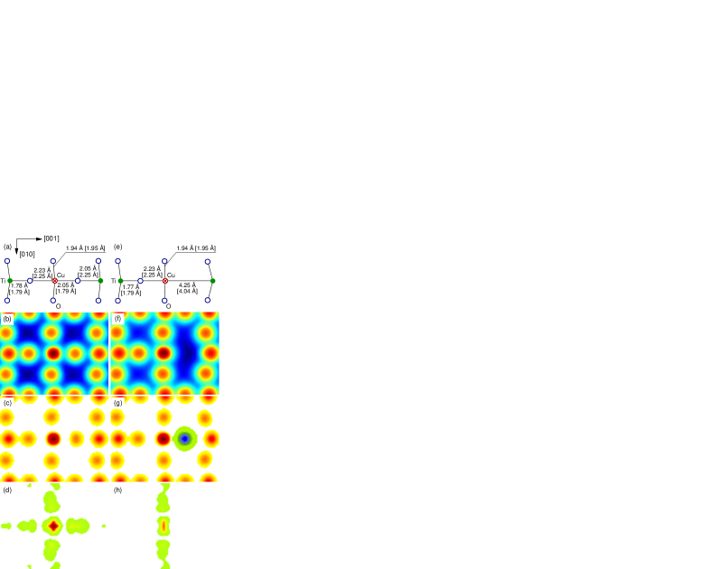
Figure 5: (Color online) Isolated copper impurity in charge state $q=-1$ (a-d) and copper impurity-oxygen vacancy complex in charge state $q=0$ (e-h). (a,e) Position of atoms in the (100)-plane containing the defect, numbers given in square brackets give the equivalent distances in the defect-free crystal; (b,f) total charge density, a logarithmic scale has been chosen for the charge density in order to enhance the features, (c,g) difference between total charge density of defective cell and defect-free cell, and (d,h) spin densities.

The partial and total densities of states for a neutral ($q=0$) copper impurity in comparison with the ideal (defect-free) system are shown in Fig. 4. The bottom of the conduction band is predominantly composed of Ti–3d orbitals (feature A in Fig. 4). Since in this energy range the contribution Cu–3d orbitals is practically zero, copper substitution leads to an effective reduction of the density of states at the bottom of the conduction band. With regard to the top of the valence band, the most obvious feature is a hybridization of Cu–3d orbitals with O–2p orbitals (feature B in Fig. 4) while the contribution of Cu-4s and Cu–3p states is negligible. In addition, a Cu-induced state emerges attached to the valence band edge (feature C in Fig. 4). As electrons are added to the system, this defect induced state is, however, shifted into the band gap because the excess charge is localized in a small volume around the defect. As a result the local potential at the copper atom is modified and an energy offset of the electronic states of this defect is induced.

Integrating the density of states and the occupied levels up to the valence band edge and including the defect induced peak, reveals three empty levels (holes) for the neutral charge state. As electrons are added to the system ($q<0$) these empty states are gradually filled. For the charge state $-1$ there are two holes localized at the Cu atom. The situation is thus equivalent to placing a $\text{Cu}^{++}$ on a Ti-site giving $\text{Cu}_{\text{Ti}}^{{}^{\prime\prime}}$, while for $q=-2$ there is one unoccupied valence band level corresponding to $\text{Cu}_{\text{Ti}}^{{}^{\prime\prime\prime}}$ ($\text{Cu}^{+}$ on $\text{Ti}^{4+}$). If the Fermi level is located in the middle of the band gap, the most stable defect is $\text{Cu}_{\text{Ti}}^{{}^{\prime\prime\prime}}$.

The $-1/-2$ transition can be understood as a local reduction of copper: The transition from charge state $q=-1$ to $q=-2$ is equivalent to the reaction $\text{Cu}^{++}+e^{-}\rightarrow\text{Cu}^{+}$. Experimentally, the redox potential for this reaction has been measured in aqueous solution to be $+0.16\,\text{eV}$ with respect to the standard hydrogen electrode, which on an absolute energy scale is located at 4.5 eV. Trasatti (1990) Thus, the $\text{Cu}^{++}/\text{Cu}^{+}$ redox potential is 4.7 eV. On the other hand, the electron affinity of PbTiO₃ is 3.5 eV and the band gap is about 3.4 eV (Ref. Robertson and Chen, 1999 and references therein) placing the valence band maximum (VBM) 6.9 eV below the vacuum level. In analogy, the redox reaction occurs roughly in the middle of the band gap (1.2 eV below the CBM or 2.2 eV above the VBM), which is in good agreement with the present calculations which locate the $-1/-2$ (or $\text{Cu}^{++}/\text{Cu}^{+}$) transition level near the mid gap. This analogy has, however, merely a qualitative character.

In order to obtain a measure for the spin-polarization of copper defects we calculated the difference between the number of electrons in spin-up and spin-down states ($\Delta n_{\upharpoonleft\downharpoonright}$ in Table 2). In both relevant charge states ($q=-1$ and $-2$) unpaired electrons are present in the system which allows to probe the defect center spectroscopically.

The geometry and charge density of an isolated copper impurity in charge state $q=-1$ is shown in Fig. 5. In comparison with the ideal crystal, copper substitution causes the $B$-site to move towards the oxygen (100)-plane. For the charge state $q=-1$ ($q=-2$) the relative displacement of the copper atom with respect to its in-plane oxygen neighbors is 0.15 Å (0.19 Å) along $[001]$, compared to 0.28 Å in the defect free crystal. Copper substitution thus causes a relaxation of the $B$-site atom in the direction of the nearest oxygen plane. The charge density plots show that the defect charge (Fig. 5(c)) as well as the spin-asymmetry (Fig. 5(d), also compare Fig. 4) is localized at the copper atom. In addition, the difference between the spin-densities in the $(100)$-plane reveals a slight asymmetry with respect to the tetragonal axis. Analysis of the electron and spin density at farther atoms – in particular the nearest Pb atoms in the $(110)$-plane – indicates that both of them are virtually unaffected by the presence of the Cu impurity.

III.1.2 Copper-vacancy complexes

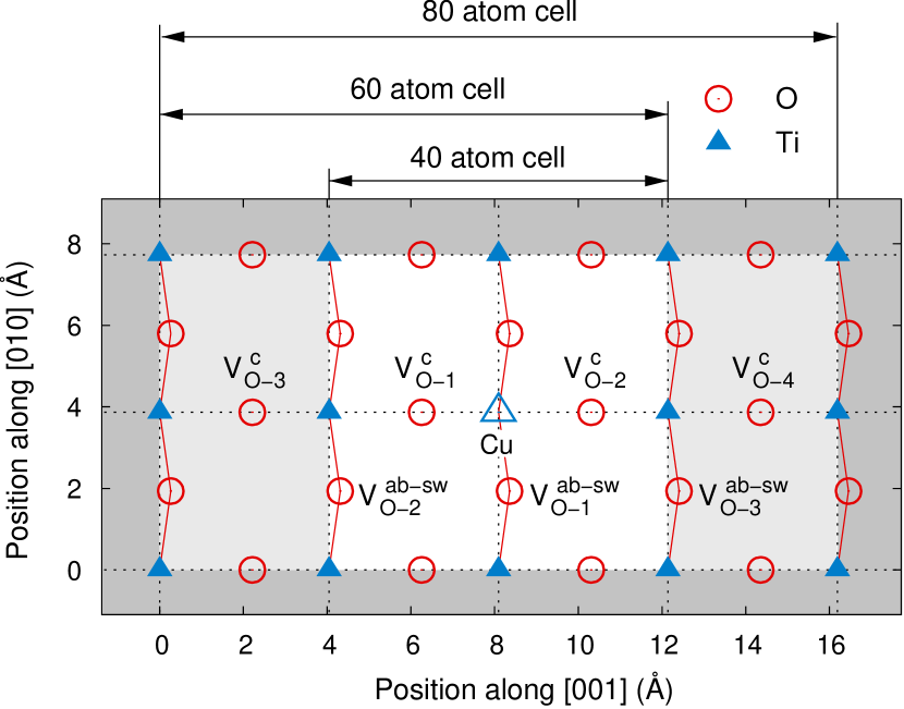
Figure 6: (Color online) Schematic of different conceivable vacancy-impurity atom configurations. The tetragonal perovskite lattice is shown along the $[100]$ axis and Pb atoms have been omitted for clarity. The different gray shaded areas indicate the size of the different supercells employed in the present work.

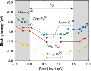
Figure 7: (Color online) Binding energies for Cu impurities in tetragonal lead titanate obtained from the extrapolated formation energies given in Tables 1 and 2. Negative energies imply a chemical driving force for association.

As illustrated in Fig. 6 different configurations for defect associates of oxygen vacancies with $B$-site impurities are conceivable. Since the impurity atom breaks the translational symmetry along the $c$-axis, the degeneracy of the positions above and below the impurity atom is lifted. In the first neighbor shell one can distinguish configurations in which the oxygen vacancy is placed along the $c$-axis either below ($M_{\text{Ti}}-V_{c}^{(1)}$, shorter $M_{\text{Ti}}-\text{O}$ distance) or above the impurity atom ($M_{\text{Ti}}-V_{c}^{(2)}$, longer $M_{\text{Ti}}-\text{O}$ distance), or on one of the four symmetry equivalent sites within the $ab$-plane ($M_{\text{Ti}}-V_{ab}$). If one considers the second-nearest neighbor shell, another two configurations involving $c$-type vacancies are possible ($M_{\text{Ti}}-V_{c}^{(3)}$, $M_{\text{Ti}}-V_{c}^{(4)}$). Further configurations are obtained by placing the vacancy on second-nearest neighbor $ab$-sites (e.g., $M_{\text{Ti}}-V_{ab}^{(2)}$ and $M_{\text{Ti}}-V_{ab}^{(3)}$ in Fig. 6). In the present work, we have considered first and second-nearest neighbor configurations involving $c$-type vacancies as well as first-nearest neighbor configurations with $ab$-vacancies. Exploratory calculations were also carried out for second-nearest neighbor $ab$-type vacancy associates. This possibility was, however, not pursued further, since the total energies were significantly larger than for the respective lowest energy configuration.

The $\text{Cu}_{\text{Ti}}-V_{c}^{(1)}$ complex, in which the vacancy is located at the nearest oxygen site along the $c$-axis (compare Fig. 6 and Fig. 5), is the most stable configuration. The most stable charge state is $q=0$ as expected if one combines $V_{\text{O}}^{\scriptscriptstyle{\bullet}\scriptscriptstyle{\bullet}}$ (see Fig. 2) and $\text{Cu}_{\text{Ti}}^{{}^{\prime\prime}}$. The energy difference with respect to the less stable complexes ($[\text{Cu}_{\text{Ti}}-V_{ab}]^{\times}$ and $[\text{Cu}_{\text{Ti}}-V_{c}^{(3)}]^{\times}$) is rather large ($0.8$-$1.0\,\text{eV}$). This large energy difference is particular noteworthy since previous model calculations assumed a much smaller energy difference on the order of 0.06 eV (compare Ref. Arlt and Neumann, 1988).

It is very instructive to compare the charge densities for isolated and complexed copper impurities. As shown in Fig. 5(d), the spin density for the isolated copper impurity is symmetric with respect to four-fold rotations about the [001] axis. This symmetry also applies for the copper-vacancy complex [Fig. 5(h)] but in addition the spin density pattern contains a (001) mirror plane through the Cu site. As can be seen by comparison of Figs. 5(a) and (e) this distinction results from the shift of the Cu atom which in the presence of a vacancy on the nearest O-site relaxes almost completely into the (001) plane of oxygen atoms leading to a local pseudo-cubic environment. These observations have important implications for the interpretation of electron paramagnetic resonance measurements as discussed in Ref. EicErhTra07, .

Finally, one can use the formation energies of isolated oxygen vacancies, copper impurities and their complexes to derive the binding energy and its dependence on the Fermi level. As shown in Fig. 7, there is a very strong chemical driving force for association of copper impurities with oxygen vacancies irrespective of the Fermi levels. If there are more oxygen vacancies than copper impurities in the system, all copper impurities will be complexed. In the opposite scenario all oxygen vacancies would be complexed and the number of isolated copper impurities would be reduced by the number of metal impurity-oxygen vacancy associates.

III.1.3 Iron impurities

Table 3: Formation energies (LSDA) in units of eV for isolated and complexed Fe-impurities on Ti-sites ($\text{Fe}_{\text{Ti}}$) in tetragonal lead titanate for a Fermi level at the valence band maximum ($\mu_{e}=0\,\text{eV}$) and metal-rich conditions ($\Delta\mu_{\text{Pb}}=\Delta\mu_{\text{Ti}}=\Delta\mu_{\text{Fe}}=0\,\text{eV}$). The finite-size scaling extrapolation errors are given in brackets in the last but one column. $\Delta n_{\upharpoonleft\downharpoonright}$ denotes the difference between the number of electrons in spin-up and spin-down states.

Defect		$\boldsymbol{\Delta n_{\upharpoonleft\downharpoonright}}$	$\boldsymbol{40}$	$\boldsymbol{60}$	$\boldsymbol{80}$	extrapolated
$\text{Fe}_{\text{Ti}}$
	$-2$	$0$	$8.64$	$8.81$	$8.87$	$9.11$	$(0.04)$
	$-1$	$1$	$7.14$	$7.18$	$7.21$	$7.27$	$(<0.01)$
	$0$	$2$	$6.26$	$6.23$	$6.23$	$6.19$	$(0.01)$
	$+1$	$3$	$6.15$	$6.12$	$6.10$	$6.05$	$(<0.01)$
$\text{Fe}_{\text{Ti}}-V_{ab}$
	$-2$	$0$	$8.69$	$8.91$	$8.96$	$9.25$	$(0.07)$
	$-1$	$1$	$6.94$	$6.99$	$7.01$	$7.08$	$(<0.01)$
	$0$	$2$	$5.46$	$5.44$	$5.44$	$5.41$	$(0.02)$
	$+1$	$3$	$4.49$	$4.43$	$4.40$	$4.31$	$(<0.01)$
	$+2$	$4$	$4.18$	$4.14$	$4.09$	$4.01$	$(0.04)$
$\text{Fe}_{\text{Ti}}-V_{c}^{(1)}$
	$-2$	$0$	$8.42$	$8.52$	$8.53$	$8.65$	$(0.05)$
	$-1$	$1$	$6.50$	$6.52$	$6.53$	$6.56$	$(<0.01)$
	$0$	$2$	$5.00$	$4.93$	$4.93$	$4.84$	$(0.04)$
	$+1$	$3$	$3.99$	$3.88$	$3.85$	$3.70$	$(0.02)$
	$+2$	$4$	$3.82$	$3.73$	$3.68$	$3.54$	$(0.02)$
$\text{Fe}_{\text{Ti}}-V_{c}^{(2)}$
	$-2$	$0$	$8.61$	$9.08$	$9.43$	$10.20$	$(0.13)$
	$-1$	$1$	$6.83$	$7.17$	$7.39$	$7.92$	$(0.06)$
	$0$	a	$5.40$	$5.60$	$5.46$	$5.62$	$(0.27)$
	$+1$	a	$4.34$	$4.25$	$4.25$	$4.15$	$(0.05)$
	$+2$	$4$	$4.09$	$4.16$	$4.17$	$4.25$	$(0.03)$
$\text{Fe}_{\text{Ti}}-V_{c}^{(3)}$
	$-2$	$0$		$9.19$	$9.11$	$8.86$
	$-1$	$0$		$6.97$	$6.87$	$6.55$
	$0$	$0$		$5.26$	$5.21$	$5.07$
	$+1$	$1$		$4.32$	$4.23$	$3.96$
	$+2$	$2$		$4.24$	$4.10$	$3.69$
$\text{Fe}_{\text{Ti}}-V_{c}^{(4)}$
	$-2$	$0$			$9.42$
	$-1$	$0$			$7.21$
	$0$	$0$			$5.55$
	$+1$	$1$			$4.54$
	$+2$	$2$			$4.27$
a The difference between electrons in spin-up and spin-down states, $\Delta n_{\upharpoonleft\downharpoonright}$, for the configuration with the lowest energy is system size dependent.

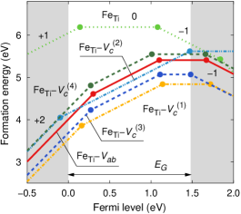
Figure 8: (Color online) Fermi level dependence of formation energies of free and complexed Fe impurities. Parallel lines imply equal charge states as indicated in the plot. The white stripe indicates the (calculated) band gap while the gray stripes indicate the valence and conduction bands, respectively. Extrapolated formation energies from Table 3 were used except for $\text{Fe}_{\text{Ti}}-V_{c}^{(4)}$ for which the data obtained with 80-atom cells are shown.

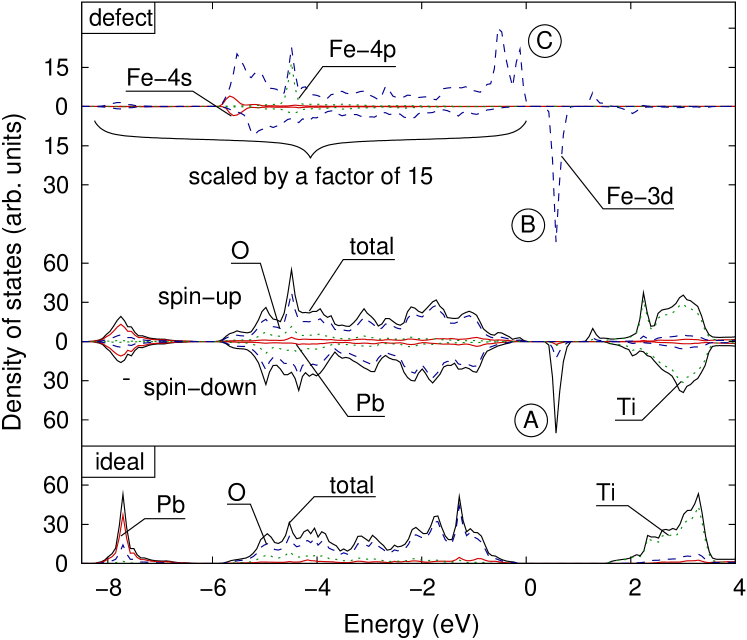
Figure 9: (Color online) Spin-decomposed total and partial density of states for neutral uncomplexed Fe impurities in lead titanate. The partial densities of states for the Fe-d orbitals are shown separately in the upper part of the figure. The Fe-s and Fe-p states have been omitted since in the energy window shown they are practically zero. A Gaussian filter with $\sigma=0.05\,\text{eV}$ was employed to smoothen the data.

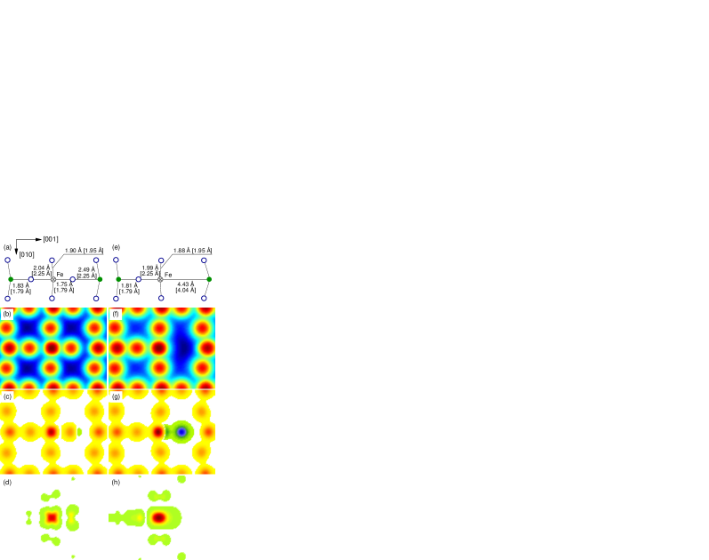
Figure 10: (Color online) Isolated iron impurity in charge state $q=0$ (a-d) and iron impurity-oxygen vacancy complex in charge state $q=+1$ (e-h). (a,e) Position of atoms in the (100)-plane containing the defect, numbers given in square brackets give the equivalent distances in the defect-free crystal; (b,f) total charge density, a logarithmic scale has been chosen for the charge density in order to enhance the features, (c,g) difference between total charge density of defective cell and defect-free cell, and (d,h) spin densities.

The formation energies for uncomplexed Fe impurities are compiled in Table 3 and presented as a function of the Fermi level in Fig. 8. The uncomplexed iron impurity occurs predominantly in the neutral charge state ($q=0$). Transition levels are only present near the band edges. It is noteworthy that according to Fig. 8 uncomplexed Fe should display ambipolar behavior. Analysis of the total and partial density of states shows that iron induces a defect level which for the neutral charge state is located in the middle of the band gap (feature A in Fig. 9). The density of states for the two different spin orientations differ considerably. While one spin-orientation (spin-down in Fig. 9) gives rise to a level in the band gap (feature B in Fig. 9), the other one leads to additional states at the top of the valence band (feature C in Fig. 9). As in the case of copper, strong hybridization occurs between the impurity atom 3d-orbitals and the O–2p levels of the host material. Also, in equivalence to copper Fe–3d levels do practically not contribute to the conduction band, slightly diminishing the density of states at the bottom of this band. Due to the presence of gap states defect induced holes and electrons cannot be unambiguously identified. In contrast to copper, a simple correlation between the Kröger-Vink notation for defects and the charge states, $q$, is, therefore, not possible.

The potentials for the redox reactions $\text{Fe}^{3+}+e^{-}\rightarrow\text{Fe}^{++}$ and $\text{Fe}^{++}+2e^{-}\rightarrow\text{Fe}^{0}$ have been measured in aqueous solution to be 0.77 eV and $-0.41\,\text{eV}$, respectively. Based on these values and using the data for the electron affinity and the band gap cited above, one would expect transition levels at 1.6 eV ($\text{Fe}^{3+}/\text{Fe}^{++}$, i.e. $\text{Fe}_{\text{Ti}}^{{}^{\prime}}/\text{Fe}_{\text{Ti}}^{{}^{\prime\prime}}$) and 2.8 eV ($\text{Fe}^{++}/\text{Fe}^{0}$, i.e. $\text{Fe}_{\text{Ti}}^{{}^{\prime\prime}}/\text{Fe}_{\text{Ti}}^{4^{\prime}}$) with respect to the experimental valence band maximum. In contrast, the present calculations indicate transitions about 0.15 eV above the VBM and 0.39 eV below the CBM. The analogy with the behavior of ions in solution, which worked reasonably in the case of copper, thus appears to fail for iron.

III.1.4 Iron-vacancy complexes

The iron-vacancy complexes which are analogous to the copper-vacancy associates described in Sec. III.1.2 and Fig. 6. In agreement with earlier calculations Meštrić et al. (2005) the configuration with the shortest distance between impurity center and oxygen vacancy ($\text{Fe}_{\text{Ti}}-V_{c}^{(1)}$) is the most stable (Fig. 8). The energetic ordering of the remaining configurations is, however, somewhat different from the case of copper. This observation has implications for the migration of oxygen vacancies and is discussed in the context of point defect models in Sec. IV and Ref. Erhart et al., .

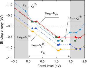
Figure 11: (Color online) Binding energies as defined by equation (2) for Fe impurities in tetragonal lead titanate obtained from the extrapolated formation energies given in Tables 1 and 3. Negative energies imply a chemical driving force for association.

The binding energies for Fe impurities shown in Fig. 11 are in general smaller than for copper and for Fermi levels very close to the valence band the binding energy can even become positive. Nonetheless for most conditions there is a rather strong ($\gg k_{B}T$) driving force for association.

Analysis of the spin density shows that for both isolated and associated iron impurities unpaired electrons are localized in the d-electron states at the iron site (Table 3). It furthermore reveals that in both cases the spin density pattern is symmetric with respect to fourfold rotations about the tetragonal axis. Unlike in the case of copper-vacancy associates the (001) plane is, however, not a mirror plane.

IV Discussion

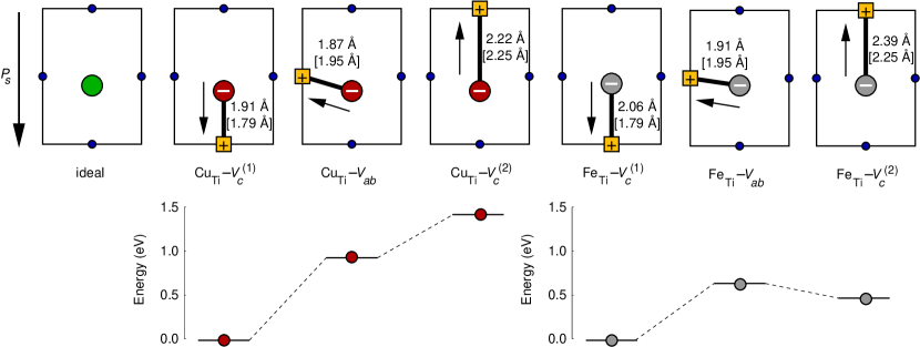
Figure 12: (Color online) Summary of key results for the most important charge states of nearest neighbor Cu/Fe-vacancy complexes ($[\text{Cu}_{\text{Ti}}-V_{\text{O}}]^{\times}$, $[\text{Fe}_{\text{Ti}}-V_{\text{O}}]^{\scriptscriptstyle{\bullet}}$). The large arrow on the far left indicates the direction of the spontaneous polarization with respect to the ideal unit cell. The short arrows indicate the direction of the defect induced dipole moments. Distances are given between the impurity atom and the position of the vacancy (as defined by the positions of the neighboring oxygen planes. Values in square brackets refer to the ideal (undistorted) lattice. The lower panel visualizes the formation energy differences.

The results obtained in this study need to be discussed in the context of degradation phenomena in ferroelectric materials. Two distinct processes have been widely described: (1) The gradual degradation of ferroelectric properties (usually over extended periods of time) in the absence of electric fields is termed “aging”. Lambeck and Jonker (1986) This process is commonly attributed to an increasing restriction of domain-wall motion with time Arlt (1987) and typically accompanied by a shift of the ferroelectric hysteresis loop along the electric field axis. Carl and Härdtl (1978); Takahashi (1982) The shift is known as the internal bias field and it has been proposed to be related to the relaxation of defect dipoles. Neumann and Arlt (1987); Arlt and Neumann (1988) In general, acceptor-doped ferroelectric ceramics with high concentrations of oxygen vacancies are particularly prone to aging. (2) The degradation of ferroelectric properties in the presence of a (usually oscillating) electric field is termed electric “fatigue”. There are various contributions to this phenomenon and possible explanations involve defects of all kinds.

The most widely known model for aging Neumann and Arlt (1987); Arlt and Neumann (1988) relates the appearance of internal bias fields to the existence and gradual reorientation of impurity-oxygen vacancy defect dipoles. Similar models have been discussed in the literature Warren et al. (1995b, 1996); Ren (2004) Experimentally, an increased internal bias field has been observed for aged lead zirconate-titanate compounds and was attributed to defect dipole alignment leading to a clamping of domain walls.Robels et al. (1992)

The availability of microscopic information on the energy landscape for defect formation and migration is the key ingredient for the these models. The present work provides a data base for these model and allow to verify their basic assumptions.

The key information regarding the orientation and the magnitude of the defect dipoles as well as their energetic ordering is summarized in Fig. 12. This picture needs to be compared to the energy landscape proposed by Arlt and Neumann Neumann and Arlt (1987); Arlt and Neumann (1988) on the basis of electrostatic arguments (Figs. 4 in Refs. Neumann and Arlt, 1987 and Arlt and Neumann, 1988). The latter analysis was carried out for barium titanate and involved several crucial assumptions with respect to e.g., the magnitude of the local dipole moment or the dielectric constant in the vicinity of the defect center. In agreement with the conclusions of the Arlt-Neumann model, the quantum-mechanical calculations show that for the energetically most stable configuration ($M_{\text{Ti}}-V_{c}^{(1)}$) the defect induced dipole is oriented parallel to the overall spontaneous polarization, $P_{s}$ (compare Fig. 12). Thus in equilibrium (i.e., a state which would be achieved after “infinite” aging) the polarization locally increases due the formation and alignment of local defect dipoles. In contrast, the defect dipole of the alternative $c$-axis configuration ($M_{\text{Ti}}-V_{c}^{(2)}$) causes a local reduction of the polarization.

In Ref. Arlt and Neumann, 1988 two estimates for the energy differences between different dipole orientations are derived. The first one treats the defect as a sphere with a defect induced polarization embedded in a ferroelectric matrix. It yields values on the order of 0.5 to 1.2 eV (compare equations (8a-8c) in Ref. Arlt and Neumann, 1988) which are of a similar magnitude as the values obtained from the present calculations. The second estimate is based on the model of an ideal point dipole and yields much smaller energy differences on the order of 0.03 to 0.06 eV (equation (9) in Ref. Arlt and Neumann, 1988). It is important to realize that the modeling of aging carried out in the same paper was actually based on the latter values.

In fact the energy differences obtained in the present work are actually on the order of magnitude of the barriers for the migration of free oxygen vacancies in this system (0.8-1.0 eV, see e.g. Ref. Park, 2003). In the vicinity of impurities the energy surface, which describes the barriers for the transformation of different defect dipole configurations into each other, is therefore severely distorted.Erhart et al. This effect is important for the behavior of defect dipoles in the presence of oscillating electric fields, which pertains to the fatigue of the material.

Finally, Fig. 12 highlights a noteworthy difference between Cu and Fe. While for Cu-complexes the energy difference between $[\text{Cu}_{\text{Ti}}-V_{c}^{(1)}]^{\times}$ and $[\text{Cu}_{\text{Ti}}-V_{c}^{(2)}]^{\times}$ is as large as $1.21\,\text{eV}$, for $[\text{Fe}_{\text{Ti}}-V_{c}^{(1)}]^{\scriptscriptstyle{\bullet}}$ and $[\text{Fe}_{\text{Ti}}-V_{c}^{(2)}]^{\scriptscriptstyle{\bullet}}$ the difference is just 0.45 eV. This difference has implications for the redistribution of the defect dipoles in the presence of an oscillating electric field and thus for the process of fatigue. A detailed account of these behavior will be published elsewhere.Erhart et al.

V Conclusions

This paper presents a comprehensive and detailed investigation of Fe and Cu dopants/impurities in tetragonal lead titanate. Both metal ions are found to be very effective traps for oxygen vacancies. In the most stable configurations the oxygen vacancy is located on a $c$-site such that the $M_{\text{Ti}}-V_{\text{O}}$ distance is minimal, and the defect dipole is aligned parallel the spontaneous polarization. This result is in qualitative agreement with an electrostatic analysis of the defect induced dipole field. An alternative configuration ($M_{\text{Ti}}-V_{c}^{(2)}$) in which the dipole is oriented anti-parallel with respect to the spontaneous polarization is somewhat higher energy but is anticipated to be of importance for the fatigue of lead titanate based ferroelectrics.

Since all relevant defects considered in this investigation carry unpaired electrons, they are visible for electron spectroscopic methods. In fact, by means of analyzing the spin density patterns for different defects it was possible to interpret recent electron paramagnetic resonance measurements and to resolve an apparent disagreement between experiment and calculations.EicErhTra07 The results obtained in this study represent important information on the energy landscape for energy formation and association and provide the basis for the improvement of defect models for the degradation of ferroelectric materials.