Dissipative vortex solitons in 2D-lattices

Abstract

We report the existence of stable symmetric vortex-type solutions for two-dimensional nonlinear discrete dissipative systems governed by a cubic-quintic complex Ginzburg-Landau equation. We construct a whole family of vortex solitons with a topological charge $S=1$. Surprisingly, the dynamical evolution of unstable solutions of this family does not alter significantly their profile, instead their phase distribution completely changes. They transform into two-charges swirl-vortex solitons. We dynamically excite this novel structure showing its experimental feasibility.

The study of discrete nonlinear systems has been an active area of research during the last twenty years due to its broad impact in diverse branches of science and to its potential for technological applications PT ; rep1 ; rep2 ; chrinat . Until now, nonlinear optics has been the main scenario chosen to test this phenomenon, essentially because of both, its comparative experimental simplicity and its direct connection with theoretical models. Nonlinear self-localized structures, usually termed as discrete solitons, have been predicted and observed for one- and two-dimensional arrays heis ; fleis . A discrete vortex soliton is defined as a nonlinear self-localized structure whose phase changes $2\pi S$ radians azimuthally. $S$ is an integer number known as the vorticity or topological charge of the solution. The existence of discrete vortex solitons in conservative systems have been reported on several works vortex1 . For the continuous case, dissipative vortex soliton families have been found to be stable for a wide interval of $S$-values opex09 . Very recently, symmetric stable vortices have also been predicted in continuous dissipative systems with a periodic linear modulation contiperio .

Nowadays, dissipative models offer a more complete and realistic description of different physical systems. In conservative models, gain and loss are completely neglected and the dynamical equilibrium is reached by means of a balance between nonlinear and dispersive effects. For dissipative systems, it must also exist an additional balance between gain and losses, turning the equilibrium into a more complex process soto . The Ginzburg-Landau equation is - somehow - a universal model where dissipative solitons are their most interesting solutions. This model appears in many branches of science like, for example, nonlinear optics, Bose-Einstein condensates, chemical reactions, superconductivity and many others akhm0508 .

In this work we deal with discrete vortex solitons in dissipative 2D lattices governed by a discrete version of the Ginzburg-Landau equation. We have found different families of these localized solutions connected successively by means of saddle-node bifurcations. We studied their stability and found two types of stable vortex families coexisting for the same set of parameters. We have dynamically unveiled the second type of stable solution by following the decaying of an initially unstable vortex. This observation is very different to the results shown in Ref. contiperio , where an unstable vortex just vanishes on propagation, through completely radiative decay. Moreover, our final vortex solution possesses a nontrivial phase structure where two different charges coexist.

Beam propagation in 2D dissipative waveguide lattices can be modeled by the following equation:

$$i\dot{\psi}_{m,n}+\hat{C}\psi_{m,n}+|\psi_{m,n}|^{2}\psi_{m,n}+\nu|\psi_{m,n}|^{4}\psi_{m,n}=$$

$$i\delta\psi_{m,n}+i\varepsilon|\psi_{m,n}|^{2}\psi_{m,n}+i\mu|\psi_{m,n}|^{4}\psi_{m,n}\ .$$ (1)

Eq.(1) represents a physical model for open systems that exchange energy with external sources and it is called $(2+1)$ discrete complex cubic-quintic Ginzburg-Landau equation. $\psi_{m,n}$ is the complex field amplitude at the $(m,n)$ lattice site and $\dot{\psi}_{m,n}$ corresponds to its first derivative respect to the propagation coordinate $z$. The set $\{m=1,...,M\}\times\{n=1,...,N\}$ defines the array, being $N$ and $M$ the number of sites in the horizontal and vertical directions (in all our computations $N=M=17$). The fields propagating in each waveguide interact only with nearest-neighbors through their evanescent tails. This interaction is described by the discrete diffraction operator $\hat{C}\psi_{m,n}=C(\psi_{m+1,n}+\psi_{m-1,n}+\psi_{m,n+1}+\psi_{m,n-1})$, where $C$ is a complex number. Its real part indicates the strength of the coupling between different sites and its imaginary part denotes the gain or loss originated by this coupling. The nonlinear higher order Kerr term is represented by $\nu$ while $\varepsilon>0$ and $\mu<0$ are the coefficients for cubic gain and quintic losses, respectively. Linear losses are determined by negative $\delta$.

Unlike the conservative discrete nonlinear Schr$\ddot{\text{o}}$dinger (DNLS) equation, the power defined as

$$Q(z)=\sum_{m,n=1}^{M,N}\ |\psi_{m,n}(z)|^{2},$$ (2)

is not a conserved quantity in the present model. However, for a self-localized solution, the power and its evolution will be the main magnitude that we will monitor in order to identify different families of stationary solutions.

We look for stationary solutions of Eq.(1) of the form $\psi_{m,n}(z)=\phi_{m,n}\exp[i\lambda z]$ where $\phi_{m,n}$ are complex numbers and $\lambda$ is real; also we are interested that the phase of solutions change azimuthally an integer number ($S$) of $2\pi$. In such a case the self-localized solution is called a discrete vortex soliton kevre2005 with vorticity $S$. By inserting the previous ansatz into model (1) we obtain the following set of algebraic coupled equations:

$$-\lambda\phi_{m,n}+\hat{C}\phi_{m,n}+|\phi_{m,n}|^{2}\phi_{m,n}+\nu|\phi_{m,n}|^{4}\phi_{m,n}=$$

$$i\delta\phi_{m,n}+i\varepsilon|\phi_{m,n}|^{2}\phi_{m,n}+i\mu|\phi_{m,n}|^{4}\phi_{m,n}\ .$$ (3)

We look for vortex-type solutions by solving equations (3) with a multi-dimensional Newton-Raphson iterative algorithm. The method requires an initial guess that we construct as explained below.

In the high-confinement limit, single peak solutions (fundamental bright solitons) were predicted to exist in dissipative nonlinear media efre07 . In that limit, we obtain the following approximation: $\phi_{0}^{2}\approx-(\varepsilon+\sqrt{\varepsilon^{2}-4\mu\delta})/(2\mu)$, $\lambda\approx\phi_{0}^{2}+\nu\phi_{0}^{4}$, and $\alpha\approx|C\phi_{0}/(\lambda+i\delta)|$. Here, $\phi_{0}$ corresponds to the central amplitude, $\lambda$ the nonlinear propagation constant, and $\alpha$ the first adjacent amplitudes. We can see from the above that the amplitude of each peak is a function of $\varepsilon$, $\mu$ and $\delta$; if we set the last two parameters, the amplitude takes a $bi$-quadratic form with $\varepsilon$ as the bifurcation parameter. Now, we place a single peak approximation at each corner of a square sub-lattice $L$ as a superposition of four fundamental bright solitons kivshar2005 :

$$L =\begin{bmatrix}0\quad&\quad\alpha\quad&\quad 0\quad&\quad\alpha\quad&\quad 0\\ \alpha\quad&\quad\phi_{0}\quad&\quad\tilde{\alpha}\quad&\quad\phi_{0}\quad&\quad\alpha\\ 0\quad&\quad\tilde{\alpha}\quad&\quad 0\quad&\quad\tilde{\alpha}\quad&\quad 0\\ \alpha\quad&\quad\phi_{0}\quad&\quad\tilde{\alpha}\quad&\quad\phi_{0}\quad&\quad\alpha\\ 0\quad&\quad\alpha\quad&\quad 0\quad&\quad\alpha\quad&\quad 0\\ \end{bmatrix},$$ (4)

where $\tilde{\alpha}=2\alpha$. Now, we define a phase operator $\Theta$ as $\Theta_{m,n}=\exp\{i{[\arctan({-n/m})]}\}$, and write our initial $S=1$ ansatz as

$$\phi_{m,n}=L_{m,n}\cdot\Theta_{m,n}\ .$$

With this initial guess, we construct a family of 4-peaks symmetric vortex solitons with vorticity $S=1$, whose stability is monitored through a standard linear stability analysis stabi . Figure 1(a) shows a $Q$ versus $\varepsilon$ diagram for these solutions including their stability. This figure shows the coexistence, for the same set of parameters, of two different branches of stable solutions and, also, three different families of unstable solitons. Different families are successively connected by saddle-node bifurcation points. An example for a solution of branch A is shown in Figs.1(b) and (c) [black dot in Fig.1(a)].

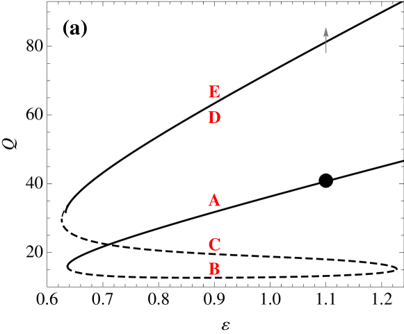
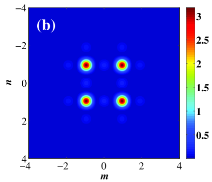
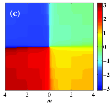
Figure 1: (Color online) (a) $Q$ versus $\varepsilon$ diagram for discrete vortex solitons. Continuous and dashed lines correspond to stable and unstable solutions, respectively. (b) and (c) Color map plots for the amplitude and phase profiles, respectively, of the solution for $\varepsilon=1.1$ indicated by a black dot in (a). $C=0.8$, $\delta=-0.9$, $\mu=-0.1$, $\nu=0.1$.

This solution is very similar to our initial ansatz sketched in Eq.(4) with a full topological charge $S=1$. This agreement validates the seed we constructed as a first approach to find stationary vortex-type solutions. As the nonlinear amplification is diminished, the stable branch $A$ reaches a first saddle-node point for $\varepsilon\approx 0.637$. At this point, this family turns around and a new family emerges: the unstable branch labeled $B$. After that, two more saddle-node points appear connecting the new branches $B$ with $C$ and, then, $C$ with $D$. The unstable branch $D$ is mostly hidden because it is located at the same region that the stable branch labeled $E$. Branches $A-D$ preserve the vorticity $S=1$ while the amplitude profiles change adiabatically. It is worth mentioning that branches $A$, $D$ and $E$ also exist for higher $\varepsilon$ values, with the power increasing monotonically, as the high-confinement limit predicts.

As said before, in Fig.1(a), curves $D$ and $E$ are indistinguishable. In order to see their differences more clearly, we plot a zoom in Fig.2(a) of region $Q\sim 81.2$ for a narrow region around the gray arrow in the Fig.1(a). The first solution on branch $E$ [black dot in Fig.2(a)] was obtained dynamically; i.e., we numerically integrated Eq.(1) by using an unstable solution [gray dot in Fig.2(a)] as initial condition. Contrary to previous observations, for the evolution of unstable vortex solitons contiperio , we noticed that the power $Q$ makes one oscillation and then stabilizes very rapidly around a new equilibrium value [see Fig.2(b)]. This new value was indeed very close to the initial one, but now it corresponds to a new stationary solution that propagates stably by keeping the same amplitude profile but a different phase structure. We took this new solution as an initial guess in our Newton-Raphson scheme and we constructed the whole stable branch $E$ shown in Fig.1(a).

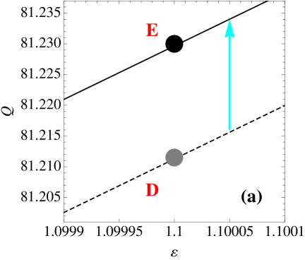
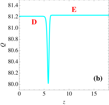
Figure 2: (Color online) (a) Zoom of branches $D$ and $E$ for a narrow region around the gray arrow in the Fig.1(a). (b) Numerical simulation of model (1) showing the power transition sketched by an cyan arrow in (a) for $\varepsilon=1.1$.

The amplitude profile for solutions corresponding to the gray and black points at Fig.2(a) is shown in Fig.3(a). This profile is almost identical for both solutions and it corresponds to a new structure that we define as “swirl-vortex soliton”. However, both solutions have a quite different phase profile. The unstable solution (belonging to branch $D$) possesses a full phase profile with charge $S=1$ [see Fig.3(b)]. A very interesting thing related with charges happens with the stable swirl-vortex soliton [see Fig.3(c)]. For the first square contour [the innermost discrete square trajectory on the plane $(n,m)$] we can see that the vorticity has a $S=1$ value, while for the next contours the vorticity has decreased to $S=-3$ [$S>0$ ($S<0$) means a clockwise phase structure from $-\pi$ to $\pi$ ($\pi$ to $-\pi$)]. Therefore, there is a stable coexistence of two different topological charges for the same mode. This new type of structure would correspond to a “two-charges swirl-vortex soliton” and - as far as we know - this would be the first time they are predicted in nonlinear lattices.

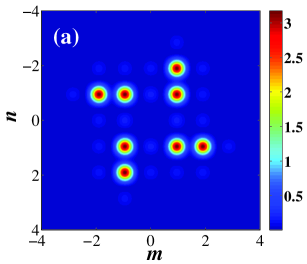
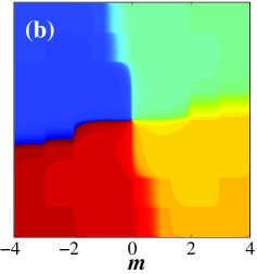
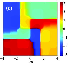
Figure 3: (Color online) Color map plots for the solutions indicated with dots in Fig.2(a). (a) Amplitude profile. (b) and (c) Phase profiles for the gray and the black points, respectively.

In order to go deeper in the understanding of this stabilization process and its dependence with the phase structure, we found another example in which the change in vorticity is also related to the stabilization of the solution. As an initial ansatz, we constructed (in the same way as the four-peaks vortex) a symmetrically-centered twenty peaks $S=1$ configuration. From the Newton-Raphson scheme we obtain an unstable vortex solution with the amplitude and phase profiles shown in Figs.4(a) and (b), respectively. Again, we use this solution as an initial condition and numerically integrate Eq.(1). As a consequence of the larger number of excited sites, the power of this solution is higher, namely $Q=202.43$. Similar to the swirl-vortex case, the solution evolves and converges to a stable solution with a very similar amplitude profile, but with a very different phase structure. For this case, the topological charge of the solution transforms from $S=1$ into $S=-3$. It is worth to mention that there is a mismatch between the vorticity of the first and next contours of the lattice [see Fig.4(c)].

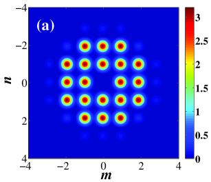
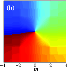
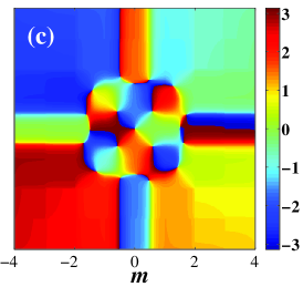
Figure 4: (Color online) Color map plots for the twenty peaks vortex solution. (a) Amplitude profile. (b) and (c) Phase profiles for the unstable $S=1$ and the stable $S=-3$ solutions, respectively. $C=0.8$, $\delta=-0.9$, $\mu=-0.1$, $\nu=0.1$ and $\varepsilon=1.1$.

Looking at the colormaps for the stable vortex soliton shown in Figs.1(b) and (c) we can realize that amplitude and phase structures have the same reflection and rotation symmetries. Similar happens with Figs.3 and Figs.4. As it was shown in previous works the stability for one solution with a high number of excited sites requires an increment of its topological charge kevre2005 ; terh . From this we understand why the dynamic evolution modify the vorticity of our solutions. So,we may conclude that the instability for complex-structure solutions of charge $S=1$ is essentially related with the geometric distribution and the number of excited sites.

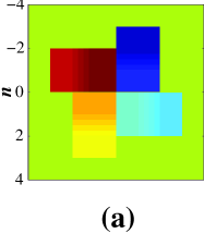
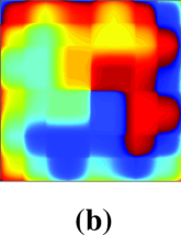
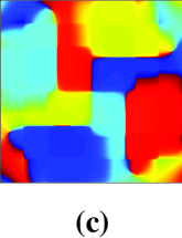
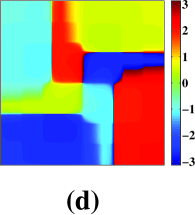
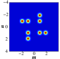
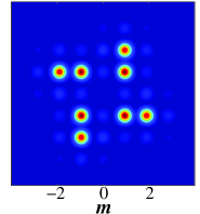
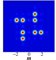
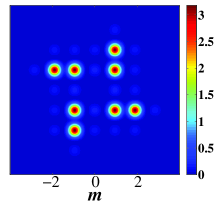
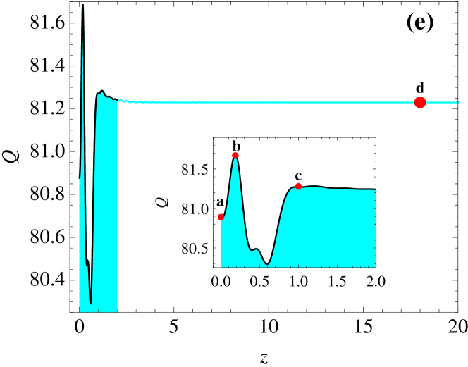
Figure 5: (a), (b), (c) and (d) Phase (upper) and amplitude (lower) profiles for different values of $z$ marked by red points in (e) where the power evolution is displayed.

We have also explored the above phenomenology in conservative-cubic systems (DNLS limit): $\delta=\mu=\nu=\varepsilon=0$. There, we found two branches of swirl-vortex solitons; one with charge $S=1$ and one with “two-charges”. The first one is always unstable while the two-charges solution is only stable for higher level of power. Here, we did not observe any decaying mechanism essentially because the system has not gain to increase the power and stabilize the solution.

Finally, and with the aim of proposing a possible experimental realization, we numerically integrate model (1) by taking - as an initial condition - a profile with eight peaks spatially distributed in the form of a swirl-vortex, including its phase structure $S=1$, as Fig.5(a) shows. With this configuration we initialize the dynamic evolution observing that the system rapidly converges to an stable stationary two-charges swirl-vortex soliton [see Figs.5(a)-(d)]. We can see that the amplitude profiles slightly change during the propagation: the eight initial peaks remain almost unaltered. On the other hand, from Figs.5(d) we see that for the first square contour the vorticity is preserved being $S=1$, while for the next contours the charge has transformed into $S=-3$. Figs.5(e) shows the evolution of power with some initially small oscillations and, lately, a tendency to the stabilization of the profile. This example shows the robustness of our prediction and its chances to be observed in real dissipative systems because the initial condition could, in principle, be easily implemented in current experimental setups. Another very interesting point is that the system naturally evolves to a “2-charges” structure. Our initial condition has an unstable phase structure which guarantees the decaying to another type of mode, but not necessarily to the one we are interested in; it could perfectly just be destroyed by the internal dynamics contiperio . However, the system favors the excitation of a swirl-vortex solution which propagates stably for long propagation distances.

In conclusion, our results reveal the existence of discrete vortex solitons in dissipative 2D-lattices. We have found stable and unstable vortices by performing different continuation methods. In particular we concentrated the study on a new type of stable structure, the so-called two-charges swirl-vortex soliton. We were able to dynamically excite it by using a simple initial configuration and therefore, believe in the feasibility of experimental observation of this novel type of dissipative structures.

C.M.C. and J.M.S.C. acknowledge support from the Ministerio de Ciencia e Innovación under contracts FIS2006-03376 and FIS2009-09895. R.A.V and M.I.M acknowledge support from FONDECYT, Grants 1080374 and 1070897, and from Programa de Financiamiento Basal de CONICYT (FB0824/2008).

References

- (1) D.K. Campbell, S. Flach, and Yu.S. Kivshar, Phys. Today 57 (1), 43 (2004).
- (2) F. Lederer, G.I. Stegeman, D.N. Christodoulides, G. Assanto, M. Segev, and Y. Silberberg, Phys. Reps. 463, 1 (2008).
- (3) S. Flach and A. Gorbach, Phys. Reps. 467, 1 (2008).
- (4) D.N. Christodoulides, F.Lederer, and Y.Silberberg, Nature (London) 424, 817 (2003).
- (5) H.S. Eisenberg, Y.Silberberg, R.Morandotti, A.R. Boyd, and J.S. Aitchison, Phys. Rev. Lett. 81, 3383 (1998).
- (6) J.W. Fleischer, M. Segev, N.K.Efrimidis, and D. N. Christodoulides, Nature (London) 422, 147 (2003).
- (7) D.N. Neshev et al., Phys. Rev. Lett. 92, 123903 (2004); J.W. Fleischer et al., Phys. Rev. Lett. 92, 123904 (2004).
- (8) J.M. Soto-Crespo, N. Akhmediev, C. Mejía-Cortés, and N. Devine, Opt. Exp. 17, 4236 (2009).
- (9) H. Leblond, B.A. Malomed, and D. Mihalache, Phys. Rev. A80, 033835 (2009).
- (10) J.M. Soto-Crespo, N. Akhmediev, and G. Town, Opt. Commun. 199, 283 (2001).
- (11) N. Akhmediev and A. Ankiewicz, Dissipative Solitons: From optics to biology and medicine, Springer, New York, 2005;
- (12) D. Pelinovsky, P. Kevrekidis, and D. Frantzeskakis, Physica D 212, 20 (2005).
- (13) N.K. Efremidis, D.N. Christodoulides, and K. Hizanidis, Phys. Rev. A76, 043839 (2007).
- (14) T.J. Alexander, A.A. Sukhorukov, and Y.S. Kivshar, Phys. Rev. Lett. 93, 063901 (2004).
- (15) R.A. Vicencio and M. Johansson, Phys. Rev. E73, 046602 (2006).
- (16) Bernd Terhalle, Tobias Richter, Kody J. H. Law et al., Phys. Rev. A79, 043821 (2009).