Free energies, vacancy concentrations and density distribution anisotropies in hard–sphere crystals: A combined density functional and simulation study

Abstract

We perform a comparative study of the free energies and the density distributions in hard sphere crystals using Monte Carlo simulations and density functional theory (employing Fundamental Measure functionals). Using a recently introduced technique (Schilling and Schmid, J. Chem. Phys 131, 231102 (2009)) we obtain crystal free energies to a high precision. The free energies from Fundamental Measure theory are in good agreement with the simulation results and demonstrate the applicability of these functionals to the treatment of other problems involving crystallization. The agreement between FMT and simulations on the level of the free energies is also reflected in the density distributions around single lattice sites. Overall, the peak widths and anisotropy signs for different lattice directions agree, however, it is found that Fundamental Measure theory gives slightly narrower peaks with more anisotropy than seen in the simulations. Among the three types of Fundamental Measure functionals studied, only the White Bear II functional (Hansen–Goos and Roth, J. Phys.: Condens. Matter 18, 8413 (2006)) exhibits sensible results for the equilibrium vacancy concentration and a physical behavior of the chemical potential in crystals constrained by a fixed vacancy concentration.

I Introduction

The phase behavior of hard spheres is one of the most intensely studied subjects within the realm of classical statistical mechanics. The existence of a fluid–solid transition has been predicted already more than fifty years ago by early computer simulation methods Woo57 ; Ald57 . Advances in colloidal engineering have led to the experimental realization of almost hard sphere–like systems, confirming the occurence of crystallization in such systems in the 1980’s Pus86 . The variety of hard sphere–like colloidal systems include polymeric spheres (index-matched solvent, sterically stabilized) Bry02 and also thermotropic colloids Sie09 using particles with diameters of the order of a few hundred nm. This allows the use of scattering techniques with visible light and/or the use of real–space microscopy to resolve single–particle positions. Using these systems and techniques, numerous features of the statics and dynamics of the crystallization process and the competing glass transition have been studied in detail (see e.g. Refs. Gas01 ; Wee02 ; Scho06 ; Zac09 ; Sch10 ).

The progress in real–space imaging opens the perspective that the static density distribution in crystals and the dynamics of the nucleation process can be studied with unprecedented resolution. The primary information obtained in these experiments, the trajectories of single particles, is very much the same as the information obtained in a computer simulation. Thus the further analysis of this primary information brings together these two fields. Currently, e.g. the processes of homogeneous and heterogeneous nucleation in colloidal hard sphere systems are under scrutiny Emm09 ; Kah09 , and the unambiguous resolution of the underlying mechanisms of these processes appears to be possible using simulation/real–space experiment on the one side and the established reciprocal–space (scattering) experiments on the other.

From the theory side, classical density functional theory (DFT) is a good candidate to study crystallization phenomena on a microscopic level. The concepts of equilibrium DFT have been developed over the past forty years (for an early review see Ref. Eva79 ). In this context, hard spheres appear to be one of the few classical fluids for which quantitatively predictive density functionals can be constructed thanks to powerful geometric arguments, leading to the so-called Fundamental Measure Theory (for recent reviews see Refs. Tar08 ; Rot10 ). In contrast to the maturity of equilibrium DFT, dynamic DFT is a still developing field which has has been started only about ten years ago Mar99 ; Arc04 ; Arc09 ; Esp09 ; Rex08 . Centerpiece of dynamic DFT is the time evolution of the inhomogeneous one–particle density. The most intensely studied variant of the theory is actually an approximation to Brownian dynamics, thus it appears to be well–suited for the study of colloidal systems. However, due to the complexity of the FMT functionals, any dynamic DFT studies of a hard sphere system with inhomogeneities in two or three dimensions have not been undertaken. In fact, there are only a few equilibrium studies of inhomogeneous problems in two and three dimensions Fri00 ; Gou01 ; Oet09 ; Bot09 , unrelated to the crystallization problem. The study of hard sphere crystals within FMT has been restricted so far to sensible parametrizations of the density distribution in a crystal, nevertheless this approach has elucidated the key features of a reliable DFT for the crystallization transition Tar00 . (A more detailed review of the problem of crystal phases within density functional theory is given below.)

In order to make progress in the direction of applying dynamic DFT (with the FMT functionals that work very well for hard spheres) to the currently studied nucleation problems Emm09 ; Kah09 , we will study first the more modest problem of the static density distribution in hard sphere crystals in this paper. This will be done by a full, three–dimensional minimization of the FMT functionals and contrasted to the results of our Monte–Carlo simulations. (Surprisingly, the density distribution in hard sphere crystals has been likewise studied very little using simulations.) Such a study is an absolute prerequisite for the more difficult dynamic problems involving crystal–fluid interfaces to be tackled in the future. We will show that the full minimization discriminates between different FMT functionals which are very similar in the description of the fluid phase. We will shed some new light on the problem of an equilibrium vacancy concentration within DFT. We will demonstrate that the FMT results for the free energy per particle for the crystal phase are in very good agreement with the corresponding simulation result which has been produced by a recently introduced method.

The paper is structured as follows. In Sec. II we briefly review the density functional approach to crystallization in the hard sphere system. Sec. III discusses a few points relevant for the FMT crystal description in more depth. These address the constrained minimization in the unit cell (with particle number fixed), the relation of the respective constrained chemical potential to Widom’s trick in a system with fixed vacancy concentration, and the numerical procedure of the FMT functional minimization. In Sec. IV we briefly describe our Monte Carlo method to obtain free energies and density distributions. Sec. V compiles our results on free energies, equilibrium vacancy concentrations and density distributions and in Sec. VI we present our conclusions.

II Hard sphere crystals in density functional theory

In density functional theory, the crystal is viewed as a self–sustained inhomogeneous fluid, i.e. an inhomogeneous density profile $\rho_{\rm cr}(\mathbf{r})$ minimizes the grand potential functional

$$\Omega[\rho(\mathbf{r})] = {\cal F}[\rho(\mathbf{r})]-\int d^{3}r\rho(\mathbf{r})\left(\mu-V^{\rm ext}(\mathbf{r})\right)\;,$$ (1)

with the external potential $V^{\rm ext}$ being zero. Here, $\mu$ is the chemical potential and ${\cal F}[\rho]$ is the free energy functional which is conventionally split into an ideal and an excess part:

$${\cal F}[\rho] = {\cal F}^{\rm id}[\rho]+{\cal F}^{\rm ex}[\rho]$$ (2)

with the exact form of the ideal part given by

$${\cal F}^{\rm id}[\rho] = \int d^{3}r\,f^{\rm id}(\mathbf{r})=\int d^{3}r\,\rho(\mathbf{r})\left(\ln[\rho(\mathbf{r})\Lambda^{3}]-1\right)\;.$$ (3)

Here, $\Lambda$ is the de–Broglie wavelength. It was realized very early (in 1979) that a simple Taylor–expanded version of the excess free energy

$${\cal F}^{\rm ex}[\rho] = \int d^{3}r\,f^{\rm ex}(\mathbf{r})\approx-\frac{1}{2}\int d^{3}r\int d^{3}r^{\prime}c^{(2)}_{\rm ref}(\mathbf{r}-\mathbf{r}^{\prime};\rho_{\rm ref})\Delta\rho(\mathbf{r})\Delta\rho(\mathbf{r}^{\prime})$$ (4)

allows for minimizing solutions $\rho_{\rm cr}(\mathbf{r})$ Ram79 . Here, $\rho_{\rm ref}$ is a reference density around the liquid coexistence density and $c^{(2)}_{\rm ref}$ is the direct correlation function in the bulk liquid at this reference density (which is related to the bulk structure factor by $S(k)=1/\rho_{\rm ref}-1/\tilde{c}^{(2)}_{\rm ref}(k)$). In this early work, the minimization to obtain $\rho_{\rm cr}$ was a constrained one: expanding the density as

$$\rho_{\rm cr}(\mathbf{r})=\rho_{0}+\sum_{j}\rho_{j}\exp({\rm i}\mathbf{K}_{j}\cdot\mathbf{r})$$ (5)

($\mathbf{K}_{j}$ is the set of the reciprocal lattice vectors), the minimization was only performed with respect to the moments $\rho_{j}$ which belong to the first or to the first and fourth shell of reciprocal lattice vectors. In this approximation, one sees that the crystal free energy in Eq. (4) “probes” the Fourier transform $\tilde{c}^{(2)}_{\rm ref}(k)$ only at one or two values of $k$. For fcc these values are $k_{1}\approx 10.9/a$ and $k_{4}\approx 20.8/a$ where $a$ is the side length of the cubic unit cell, very near the first two maxima of $\tilde{c}^{(2)}_{\rm ref}(k)$ resp. $S(k)$. At first sight, it may appear surprising that an expansion of the free energy like Eq. (4), valid at small density variations is sufficient to sustain the rapidly varying density profile in a crystal. However, the isotropic correlations between two particles in Fourier space are described by the structure factor (and hence by $c^{(2)}_{\rm ref}$). Since the shells of reciprocal lattice vectors for an fcc lattice are also distributed fairly isotropically, the possible description of a solid with a density near the reference density appears to be less unexpected. Subsequent work has revealed that the expansion in reciprocal space (5) is converging slowly. Furthermore, there are serious quantitative problems in this approach if it comes to the description of the lattice density peak width (much too narrow), crystals at higher density (unstable) and the vacancy density (around 10 percent at coexistence which is a factor of about 100 too large) Hay85 ; Jon85 .

A more general approach to inhomogeneous hard sphere fluids in general and to the description of crystals in particular consists in the ansatz

$${\cal F}^{\rm ex}[\rho]=\int d^{3}r\,\rho(r)\Psi(\bar{\rho}(\mathbf{r}))\;.$$ (6)

Here, $\Psi$ is a suitable function of a weighted density

$$\bar{\rho}(\mathbf{r})=\int d^{3}r^{\prime}\rho(\mathbf{r}^{\prime})w(\mathbf{r}-\mathbf{r}^{\prime};\bar{\rho})=\rho*w\,(\mathbf{r})$$ (7)

which employs a weight function which in turn may depend on the weighted density itself. (For the Taylor expanded functional (4), $\bar{\rho}={\rm const.}+c^{(2)}_{\rm ref}*\rho$.) The functions $\Psi$ and $w$ can be determined through the equation of state and the bulk direct correlation functions which are assumed to be known. Here, the self–consistent solution for $w$ may be rather involved in particular realizations. Examples for this class of functionals include the Tarazona functionals Mark I Tar84 and Mark II Tar85 , the weighted–density approximation (WDA) Cur85 and the modified WDA Den95 . Crystal structures in these approaches have been usually obtained by minimizing the ansatz

$$\rho_{\rm cr} = \sum_{{\rm lattice\;sites}\;i}N\,\left(\frac{\alpha}{\pi}\right)^{\frac{3}{2}}\,\exp\left(-\alpha(\mathbf{r}-\mathbf{r}_{i})^{2}\right)$$ (8)

with respect to the Gaussian peak width $\alpha$ and the normalization $N$. If $n_{\rm vac}$ denotes the relative concentration of vacancies then $N=1-n_{\rm vac}$. With such a Gaussian ansatz, the reciprocal lattice modes of the density (see Eq. (5)) are given by $\rho_{j}=N\,\exp(-\mathbf{K}_{j}^{2}/(4\alpha))$. Using the most sophisticated versions of these weighted–density approaches, one can achieve a rather good agreement with simulations for the liquid–solid coexisting densities and a physically sensible behavior also for denser crystals. This is understandable since in comparison with the simple Taylor expanded functional (4) the weighted–density form (6) includes contributions from higher–order direct correlation functions and through the self–consistent determination of $w$ it is guaranteed that at higher densities the changed isotropic correlations in a (possibly metastable) reference liquid are taken into account. Still, the lattice density peaks come out too narrow compared to simulations, the crystal free energy per particle is too small by about 5% and a quasifree minimization in modified WDA (with the restriction $n_{\rm vac}=0$) revealed qualitatively wrong peak asymmetries in the different lattice directions as well as an unphysically large interstitial density Ohn93 . A sensible, small vacancy concentration $n_{\rm vac,0}$ which minimizes the free energy can only be obtained by incorporating an appropriate additional constraint term into the free energy functional Ohn91 .

However, the WDA approach which is built on the isotropic fluid correlations cannot be expected to treat coordination effects in crystals correctly on a fundamental level. These include the description of the metastable hard sphere bcc crystal Run87 and the crystal–fluid interface Ohn94 . Here, the development of fundamental measure theory (FMT) marks an important breakthrough Ros89 . FMT postulates an excess free energy with a local free energy density in a set of weighted densities $n_{\alpha}$:

$${\cal F}^{\rm ex}[\rho] = \int d^{3}r\Phi(n_{\alpha}(\mathbf{r}))\;.$$ (9)

The weighted densities are again constructed as convolutions of the density with weight functions, $n_{\alpha}(\mathbf{r})=\rho*w^{\alpha}(\mathbf{r})$. In contrast to the WDA, the weight functions reflect the geometric properties of the individual hard spheres (and not the properties of an interacting pair). For one species, the weight functions include four scalar functions $w^{0}\dots w^{3}$, two vector functions $\mathbf{w}^{0},\mathbf{w}^{1}$ and a tensor function $w^{t}$ defined as

$$w^{3}=\theta(R-|\mathbf{r}|)\;,\qquad w^{2}=\delta(R-|\mathbf{r}|)\;,\qquad w^{1}=\frac{w^{2}}{4\pi R}\;,\qquad w^{0}=\frac{w^{2}}{4\pi R^{2}}\;,$$

$$\mathbf{w}^{2}=\frac{\mathbf{r}}{|\mathbf{r}|}\delta(R-|\mathbf{r}|)\;,\qquad\mathbf{w}^{1}=\frac{\mathbf{w}^{2}}{4\pi R}\;,$$

$$w^{t}_{ij}=\frac{r_{i}r_{j}}{\mathbf{r}^{2}}\delta(R-|\mathbf{r}|)\;.$$ (10)

Here, $R$ is the hard sphere radius. Using these weight functions, corresponding scalar weighted densities $n_{0}\dots n_{3}$, vector weighted densities $\mathbf{n}_{1},\mathbf{n}_{2}$ and one tensor weighted density $n_{t}$ are defined. In constructing the free energy density $\Phi$, arguments concerning the correlations in the bulk fluid and arguments for strongly inhomogeneous systems are used. For the bulk, $\Phi$ is required to reproduce exactly the second and third virial coefficent of the direct correlation function. Furthermore, imposition of the Carnahan–Starling equation of state Rot02 ; Yu02 and/or consistency with a scaled particle argument Ros89 ; Han06 leads to a closed form for $\Phi$. The arguments using strongly inhomogeneous systems are known in the literature under the label “dimensional crossover” Ros97 : Through a suitable external potential, the hard sphere fluid can be confined to lower dimensions and the density functionals for these lower–dimensional systems should emerge from the correct density functional in 3d. Of particular relevance are the crossover to 1d where the exact density functional is known Per76 and to 0d where a hard sphere is confined to a point and the free energy is a simple function of the mean occupation number at this point Ros97 . The 0d confinement can be realized through differently shaped cavities (overlapping spheres of radius $R$) which can hold only one particle (see Fig. 1). Respecting the 0d limit for different cavities is of particular relevance for the crystal description since this means that the mutual exclusion of hard spheres in various coordinations is correctly described. In Refs. Tar97 ; Tar00 a solution is given which respects the 0d limit for cavities (a) and (b) of Fig. 1 and approximates the 0d limit for cavity (c).

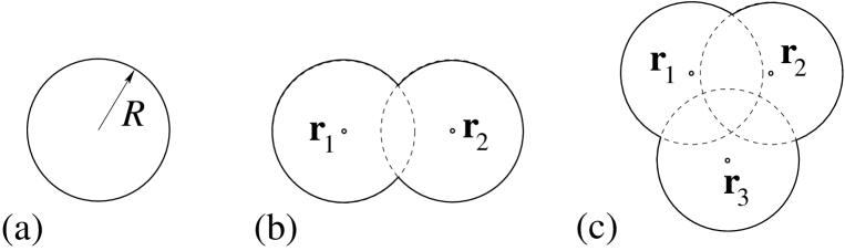
Figure 1: Three types of cavities which can hold only one particle.

The arguments presented in the above paragraph lead to the following form of the excess free energy density:

$$\Phi(\{\mathbf{n}[\rho(\mathbf{r})]\}) = -n_{0}\,\ln(1-n_{3})+\varphi_{1}(n_{3})\;\frac{n_{1}n_{2}-\mathbf{n}_{1}\cdot\mathbf{n}_{2}}{1-n_{3}}+$$ (11)

$$\varphi_{2}(n_{3})\;\frac{3\left(-n_{2}\,\mathbf{n}_{2}\cdot\mathbf{n}_{2}+n_{2,i}n_{t,ij}n_{2,j}+n_{2}\,n_{t,ij}n_{t,ji}-n_{t,ij}n_{t,jk}n_{t,ki}\right)}{16\pi(1-n_{3})^{2}}\;.$$

Here, $\varphi_{1}(n_{3})$ and $\varphi_{2}(n_{3})$ are functions of the local packing density $n_{3}(\mathbf{r})$. With the choice

$$\varphi_{1}=1\;,\qquad\varphi_{2}=1$$ (12)

we obtain the Tarazona tensor functional Tar00 which is built upon the original Rosenfeld functional Ros89 . The latter gives the fluid equation of state and pair structure of the Percus–Yevick approximation. Upon setting

$$\varphi_{1} = 1$$ (13)

$$\varphi_{2} = 1-\frac{-2n_{3}+3n_{3}^{2}-2(1-n_{3})^{2}\ln(1-n_{3})}{3n_{3}^{2}}$$

we obtain the tensor version of the White Bear functional Rot02 , consistent with the quasi–exact Carnahan–Starling equation of state. Finally, with

$$\varphi_{1} = 1+\frac{2n_{3}-n_{3}^{2}+2(1-n_{3})\ln(1-n_{3})}{3n_{3}}$$ (14)

$$\varphi_{2} = 1-\frac{2n_{3}-3n_{3}^{2}+2n_{3}^{3}+2(1-n_{3})^{2}\ln(1-n_{3})}{3n_{3}^{2}}$$

the tensor version of the recently introduced White Bear II functional Han06 is recovered. This functional is most consistent with restrictions imposed by morphological thermodynamics Koe04 .

III Hard sphere crystals in FMT

III.1 Minimization and $\mu$ consistency

The minimization of the grand potential functional

$$\Omega[\rho] = {\cal F}^{\rm id}[\rho]+{\cal F}^{\rm ex}[\rho]-\int d^{3}r(\mu-V^{\rm ext}(\mathbf{r}))\rho(\mathbf{r})\;,$$ (15)

leads to

$$\beta^{-1}\ln(\rho_{\rm eq}(\mathbf{r})\Lambda^{3})=-\mu^{\rm ex}[\rho_{\rm eq}(\mathbf{r})]+\mu-V^{\rm ext}(\mathbf{r})\;.$$ (16)

The functional $\mu[\rho(\mathbf{r})]$ is given by

$$\mu^{\rm ex}[\rho(\mathbf{r})] = \frac{\delta{\cal F}^{\rm ex}[\rho]}{\delta\rho(\mathbf{r})}$$ (17)

$$= \beta^{-1}\sum_{\alpha}\int d\mathbf{r}^{\prime}\,\frac{\partial\Phi}{\partial n_{\alpha}(\mathbf{r}^{\prime})}\,w^{\alpha}(\mathbf{r}^{\prime}-\mathbf{r})\;.$$ (18)

In principle, for a force–free system ($V^{\rm ext}=0$), the specification of a suitable chemical potential $\mu$ should lead upon minimization to a periodic crystal profile $\rho_{\rm eq}\equiv\rho_{\rm cr}(\mathbf{r})$ with the bulk density $\rho_{0}(\mu)$. The side length $a$ of the cubic unit cell and consequently the vacancy concentration $n_{\rm vac}$ should adjust itself to comply with Eq. (16). Here, $n_{\rm vac}$ is connected to the occupation of the unit cell of the fcc lattice by

$$\int_{\rm cell}d^{3}r\,\rho(\mathbf{r})=4(1-n_{\rm vac})\;.$$ (19)

In practice, such a procedure is not feasible. Rather, for a given bulk density $\rho_{0}$, also $n_{\rm vac}$ (and thus $a$) is prescribed and a constrained free energy functional for the unit cell

$$\left.\Omega^{\prime}\right|_{\rm cell}=\int_{\rm cell}d^{3}r\,{f}^{\rm id}[\rho]+\int_{\rm cell}d^{3}r\,{f}^{\rm ex}[\rho]-\mu^{\prime}\int_{\rm cell}d^{3}r\,(\rho(\mathbf{r})-\rho_{0})$$ (20)

is minimized where $\mu^{\prime}=\mu^{\prime}(\rho_{0},n_{\rm vac})$ plays the role of a Lagrange multiplier to ensure (19). In the work reviewed previously $\mu^{\prime}$ was not determined explicitly, and only a few studies bothered to vary also $n_{\rm vac}$ (which should be close to zero) such that the free energy per particle is indeed minimized. However, there is a useful consistency condition between $\mu^{\prime}$ and $\mu(\rho_{0})$. Let $f_{\rm cr}(\rho_{0})$ denote the free energy density for the fully minimized crystal with vacancy concentration $n_{\rm vac,0}$. Then

$$\mu=\frac{df_{\rm cr}}{d\rho_{0}}\stackrel{{\scriptstyle!}}{{=}}\left.\mu^{\prime}(\rho_{0},n_{\rm vac})\right|_{n_{\rm vac}=n_{\rm vac,0}}\;$$ (21)

This can be shown as follows. Let $\rho_{\rm eq}(\rho_{0},n_{\rm vac};\mathbf{r})$ be the minimizing density profile for a crystal with fixed bulk density $\rho_{0}$ and vacancy concentration $n_{\rm vac}$. Using the expansion in reciprocal lattice vectors (5), $\rho=\rho_{0}+\sum_{j}\rho_{j}\exp({\rm i}\mathbf{K}_{j}\cdot\mathbf{r})$, it is seen that the constrained minimization of Eq. (20) yields

$$\mu^{\prime}(\rho_{0},n_{\rm vac}) = \frac{1}{a^{3}(\rho_{0},n_{\rm vac})}\int_{\rm cell}d^{3}r\,\frac{\partial(f^{\rm id}[\rho_{\rm eq}]+f^{\rm ex}[\rho_{\rm eq}])}{\partial\rho_{0}}$$ (22)

$$= \frac{1}{a^{3}(\rho_{0},n_{\rm vac})}\int_{\rm cell}d^{3}r\,(\ln(\rho_{\rm eq}\Lambda^{3})+\mu^{\rm ex}[\rho_{\rm eq}])\;.$$

Here, the last line follows since $\int d^{3}r\,\partial f^{\rm ex}/\partial\rho_{0}=\int d^{3}r\,(\delta{\cal F}^{\rm ex}/\delta\rho)\,(\partial\rho/\partial\rho_{0})$ and $\partial\rho/\partial\rho_{0}=1$. On the other hand, the chemical potential from the crystal equation of state becomes:

$$\mu=\frac{df_{\rm cr}}{d\rho_{0}} = \left.\frac{\partial f_{\rm cr}}{\partial n_{\rm vac}}\;\frac{\partial n_{\rm vac}}{\partial\rho_{0}}\right|_{n_{\rm vac}=n_{\rm vac,0}}+\frac{1}{a^{3}(\rho_{0},n_{\rm vac,0})}\int_{\rm cell}d^{3}r\,\frac{\partial(f^{\rm id}[\rho_{\rm cr}]+f^{\rm ex}[\rho_{\rm cr}])}{\partial\rho_{0}}\;$$ (23)

$$= \left.\rho_{0}\frac{\partial(F_{\rm cr}/N)}{\partial n_{\rm vac}}\;\frac{\partial n_{\rm vac}}{\partial\rho_{0}}\right|_{n_{\rm vac}=n_{\rm vac,0}}+\mu^{\prime}(\rho_{0},n_{\rm vac,0})=\mu^{\prime}(\rho_{0},n_{\rm vac,0})$$

Thus we see that $\mu(\rho_{0})=\mu^{\prime}(\rho_{0},n_{\rm vac,0})$, since the crystal free energy particle per particle ($F_{\rm cr}/N$) is minimal at $n_{\rm vac}=n_{\rm vac,0}$.

III.2 Basic considerations on single defects

As we have seen in the previous considerations, the appearance of defects enters the equilibrium density profile in a crystal through the average occupation of a lattice site. The dominating type of defect in the equilibrium hard sphere crystal are monovacancies whose properties have been studied before in simulations explicitly Ben71 ; Pro01 ; Kwa08 . In order to derive a general formula for the constrained chemical potential $\mu^{\prime}(\rho_{0},n_{\rm vac,0})$ it is useful to discuss the thermodynamics of a crystal containing vacancies more in detail.

Here we follow Ref. Pro01 in the subsequent reasoning. We introduce a system with $M$ lattice sites which contains $n$ monovacancies at given positions and index thermodynamic quantities with these numbers, such that e.g. $V_{M,1}$ denotes the volume of a lattice with $M$ sites, 1 fixed vacancy and therefore $M-1$ particles. Furthermore it is convenient to define by $-f_{\rm vac}$ the change in free energy due to the creation of a single vacancy at a specific lattice point while keeping the volume and the number of lattice sites constant:

$$-f_{\rm vac} = F_{M+1,1}(M,V_{M+1,0},T)-F_{M+1,0}(M+1,V_{M+1,0},T)$$ (24)

$$= -\ln(\rho_{0}\Lambda^{3})-f_{\rm vac}^{\rm ex}\;.$$

As usual, the free energy $F(N,V,T)$ is a function of particle number $N$, volume and temperature. In the second line we have separated $-f_{\rm vac}$ into the ideal gas contribution and the excess part $-f_{\rm vac}^{\rm ex}$. Assuming no interaction between pairs of monovacancies, the total free energy $F_{M,n}$ is

$$F_{M,n}=F_{M,0}-nf_{\rm vac}=Mf_{0}-nf_{\rm vac}$$ (25)

where $f_{0}$ is the free energy per particle (or per lattice site) in a defect–free crystal (i.e. precisely the value of $F/N$ determined in our simulations). In order to calculate the equilibrium concentration of vacancies, it is more convenient to switch to the Gibbs free energy $G_{M,n}(M-n,p,T)$ in a system of $M-n$ particles at constant pressure $p$ and temperature $T$. We define $g_{\rm vac}$ as the change in $G$ due to the creation of a single vacancy at a specific lattice point:

$$g_{\rm vac} = G_{M+1,1}(M,p,T)-G_{M,0}(M,p,T)$$ (26)

$$= F_{M+1,1}(M,V_{M+1,1},T)-F_{M,0}(M,V_{M,0},T)+p(V_{M+1,1}-V_{M,0})\;.$$

Using Eq. (24) and furthermore $f_{0}=F_{M+1,0}(M+1,V_{M+1,0},T)-F_{M,0}(M,V_{M,0},T)$ and $\mu_{0}=f_{0}+pV_{M,0}/M$ we find

$$g_{\rm vac}=\mu_{0}-f_{\rm vac}\;.$$ (27)

The total Gibbs free energy $G^{\rm tot}_{M,n}$ includes the entropic contribution due to the distribution of $n$ vacancies over $M$ lattice sites ($n\ll M$):

$$G^{\rm tot}_{M,n}\approx G_{M-n,0}+ng_{\rm vac}+nk_{\rm B}T\left(\ln\frac{n}{M}-1\right)$$ (28)

Minimizing with respect to $n$ yields the equilibrium concentration of monovacancies $n_{\rm vac,0}$:

$$n_{\rm vac,0}=\frac{n}{M}=\exp(-\beta g_{\rm vac})=\exp(-\beta(\mu_{0}-f_{\rm vac}))\;.$$ (29)

Let us now define an excess chemical potential $\mu^{\prime}_{\rm Wi}(n_{\rm vac})$ for a constrained crystal at a fixed vacancy concentration $n_{\rm vac}$ through the free energy of particle insertion (Widom’s trick). Its excess part can be estimated by the probability $P_{acc}(V_{\rm WS})$ of inserting a particle into the Wigner–Seitz cell (with volume $V_{\rm WS}$) around the vacancy position and the probability $n_{\rm vac}$ of picking the vacancy lattice site among all lattice sites. Thus:

$$\mu_{\rm Wi}^{\prime}(n_{\rm vac}) \approx \ln(\rho_{0}\Lambda^{3})-k_{\rm B}T\ln\left(P_{\rm acc}(V_{\rm WS})\right)-k_{\rm B}T\ln n_{\rm vac}$$ (30)

$$= f_{\rm vac}-k_{\rm B}T\ln n_{\rm vac}$$

The second line follows since $-k_{\rm B}T\ln P_{\rm acc}(V_{\rm WS})$ is precisely the excess free energy cost $f_{\rm vac}^{\rm ex}$ of removal of one vacancy Pro01 . We see immediately that in equilibrium, $n_{\rm vac}=n_{\rm vac,0}$, we have $\mu_{\rm Wi}^{\prime}(n_{\rm vac,0})\approx\mu_{0}$ which demonstrates the consistency between the thermodynamic and insertion route in equilibrium. (Note that the correction to the equilibrium chemical potential is only linear in $n_{\rm vac,0}$ Pro01 .) However, for the constrained system the insertion route predicts that $\mu^{\prime}(\rho_{0},n_{\rm vac})$ diverges upon $n_{\rm vac}\to 0$.

The system with the constraint of fixed $n_{\rm vac}$ corresponds to the free energy functional in Eq. (20) and thus we may identify $\mu_{\rm Wi}^{\prime}(n_{\rm vac})\equiv\mu^{\prime}(\rho_{0},n_{\rm vac})$. Therefore the logarithmic increase of the chemical potential with $n_{\rm vac}\to 0$ is a stringent test for fully minimized density functional models. However, we want to point out that physically the divergence of $\mu^{\prime}$ with vanishing vacancy density is not entirely correct as outlined in the following. Even in a perfect lattice it is possible to insert another interstitial particle. Similarly to $-f_{\rm vac}$ one can define the change in free energy $f_{\rm in}$ due to the creation of a single interstitial at a specific lattice point while keeping the volume and the number of lattice sites constant:

$$f_{\rm in} = F_{M,1}(M+1,V_{M,1},T)-F_{M,0}(M,V_{M,0},T)\;.$$ (31)

The second index for $F$ and $V$ refers to the number of interstitial particles in the system. Therefore it follows that for vanishing vacancy concentration the constrained chemical potential is given by

$$\mu^{\prime}(\rho_{0},n_{\rm vac}\ll n_{\rm vac,0})=f_{\rm in}+{\cal O}(n_{\rm vac})\;.$$ (32)

Simulation results for the free energies $f_{\rm vac}$ and $f_{\rm in}$ in hard sphere crystals near coexistence give approximately the magnitudes 8 $k_{\rm B}T$ and 34 $k_{\rm B}T$, respectively Pro01 ; Kwa08 . Since $f_{\rm in}\gg f_{\rm vac}$, it is clear that the constrained chemical potential should exhibit the logarithmic divergence upon $n_{\rm vac}\to 0$ down to very small vacancy concentrations. (At coexistence, $\mu^{\prime}(\rho_{0},n_{\rm vac,0})=\mu_{0}\approx 16$ $k_{\rm B}T$. For smaller $n_{\rm vac}$, $\mu^{\prime}$ should rise up to approximately $f_{\rm in}\approx 34$ $k_{\rm B}T$ and then level off.)

III.3 Previous results in FMT

A fully three–dimensional minimization of FMT aiming at the crystal profile has not been carried out before. In Tarazona’s ground–breaking work Tar00 the density profile was parametrized as

$$\rho_{\rm cr}(\mathbf{r}) = \sum_{{\rm lattice\;sites}\;i}(1-n_{\rm vac})\,\left(\frac{\alpha}{\pi}\right)^{\frac{3}{2}}\,\exp\left(-\alpha(\mathbf{r}-\mathbf{r}_{i})^{2}\right)\,\left(1+K_{4}\alpha^{2}f_{4}(\mathbf{r}-\mathbf{r}_{i})\right)\;,$$ (34)

$$f_{4}(\mathbf{r}=(x,y,z))=x^{4}+y^{4}+z^{4}-\frac{3}{5}r^{4}\;.$$

Here, $f_{4}$ is the leading term for the unit cell anisotropy in cubic lattices. The free energy per particle was minimized with respect to $n_{\rm vac}$, $\alpha$ and $K_{4}$ using the Rosenfeld tensor functional (11) and (12). The anisotropy turned out to be unimportant for the values of $F_{\rm cr}/N$ (modifying it by less than $10^{-3}$ $k_{\rm B}T$). Both $F_{\rm cr}/N$ and $\alpha$ were shown to be in good agreement with the old simulation data of Ref. You74 . No clear free energy minimum was found for a nonzero $n_{\rm vac}$, indicating that $n_{\rm vac,0}<10^{-8}$.

Concerning the issue of the equilibrium vacancy concentration $n_{\rm vac,0}$ in FMT, there are two more, partially contradictory statements in the literature. In Ref. Ros97 it was argued that the correct 0d limit of a density functional (for particles strictly localized to their lattice sites) should always lead to a finite, but small $n_{\rm vac,0}$. The 0d excess free energy is given by $\beta F^{\rm ex}_{\rm 0d}=\eta+(1-\eta)\,\ln(1-\eta)$ with a corresponding excess chemical potential $\beta\mu^{\rm ex}_{\rm 0d}=-\ln(1-\eta)$. Since the packing fraction at each lattice site is corresponds to $1-n_{\rm vac}$, one finds $\beta\mu^{\rm ex}_{\rm 0d}=-\ln n_{\rm vac}$. The equilibrium vacancy concentration follows upon identification of $\mu^{\rm ex}_{\rm 0d}(n_{\rm vac,0})$ with the crystal chemical potential $\mu_{0}$ as $n_{\rm vac,0}=\exp(-\beta\mu^{\rm ex}_{\rm 0d})$. According to this argument one would expect an equilibrium vacancy concentration $n_{\rm vac,0}\sim 10^{-8}$ at coexistence. We observe that the divergence of $\beta\mu^{\rm ex}_{\rm 0d}$ is precisely of the type derived before for the constrained chemical potential $\mu^{\prime}(\rho_{0},n_{\rm vac})$ (see Eq. (30)). However, the plain identification $\mu^{\rm ex}_{\rm 0d}\equiv\mu^{\prime}$ is incorrect due to the neglect of the free energy of vacancy formation. This explains the four orders of magnitude difference in $n_{\rm vac,0}$ when compared with simulations Ben71 ; Kwa08 . Another approach was taken in Ref. Gro00 to calculate $n_{\rm vac,0}$. There, the Rosenfeld functional (among others) was minimized in a perturbative approach assuming isotropic density distributions around lattice sites and an expansion around the close–packing limit. A free energy minimum was found for values of $n_{\rm vac,0}$ consistent with simulation results. However, we will demonstrate below that this finding is not consistent with our full minimizations.

The success of the density parametrization using isotropic Gaussians and zero vacancy concentration inspired the works of Ref. Lut06 to investigate non-fcc crystals and of Refs. Son06 ; Son08 to treat binary systems and the crystal–fluid interface within FMT. In the latter work, the interface density profile was parametrized in an intuitive way, however, in this way one cannot ensure that crystal and fluid are in chemical equilibrium (see Sec. V below).

III.4 Numerical solution of the FMT Euler–Lagrange equation

In actual calculations, we determine the constrained crystal profile $\rho_{\rm eq}(\rho_{0},n_{\rm vac};\mathbf{r})$ by a full minimization in three–dimensional real space. For such a three-dimensional problem, the density profile $\rho$ and 11 weighted densities (two scalar densities $n_{2},\,n_{3}$, three vector densities $(\mathbf{n}_{2})_{i}$ for $i=\{x,y,z\}$ and six tensor densities $(n_{t})_{ij}$ for $\{ij\}=\{xx,yy,zz,xy,xz,yz\}$) need to be discretized on a three–dimensional grid covering the cubic unit cell. Usually we chose grids with dimensions 64³ (for lower densities around the coexistence density $\rho_{\rm coex}\sigma^{3}\approx 1.04$) up to 256³ (for higher densities). Here, $\sigma=2R$ is the hard sphere diameter. The necessary convolutions were computed using Fast Fourier Transforms. With prescribed $\rho_{0}$ and $n_{\rm vac}$, the constrained functional (20) is minimized through Picard iteration (with mixing) of the Euler–Lagrange equation (16). A new profile $\rho_{i+1}$ is determined from an old profile $\rho_{i}$ and an appropriate $\mu^{\prime}_{i}$ through

$$\rho_{i+1} = \alpha\,\rho^{\prime}_{i+1}+(1-\alpha)\,\rho_{i}\;,$$ (35)

$$\rho^{\prime}_{i+1} = \exp\left(-\beta\frac{\delta{\cal F^{\rm ex}}}{\delta\rho(\mathbf{r})}[\rho_{i}]+\beta\mu^{\prime}_{i}\right)\;.$$ (36)

Here, $\mu^{\prime}_{i}$ is determined such that $\int_{\rm cell}d^{3}r\,\rho_{i+1}=4(1-n_{\rm vac})$. The mixing parameter $\alpha$ is of the order of 0.01. The iteration was stopped when the relative deviation between $\mu^{\prime}_{i}$ and $\mu^{\prime}(\rho_{0},n_{\rm vac})$ from Eq. (22) was below $5\cdot 10^{-6}$. The iteration procedure was stabilized by two means: (i) enforcing the physical requirement $n_{3}(\mathbf{r})\leq 1-n_{\rm vac}$ at each iteration step since the singularity at $n_{3}=1$ (see the functional in Eq. (11)) is avoided in that manner. (ii) enforcing the point symmetry of the fcc crystal in the density profile in each iteration step. In each iteration, this point symmetry is slightly violated by numerical inaccuracies. Without correction and using $\alpha\sim 0.01$, this symmetry violation quickly grows and eventually leads to numerical singularities. Only for $\alpha\lesssim 10^{-5}$, convergence was achieved without explicit enforcement of the point symmetry at the price of an increase in computation time by a factor 100–1000. For a given $\rho_{0}$, $n_{\rm vac}$ is varied and the location of the minimum is checked using the consistency condition (21). However, for $n_{\rm vac}<10^{-5}$ it proved to be hard to arrive at a convergent solution.

IV Monte Carlo simulations

IV.1 Computation of absolute free energies

The computation of absolute free energies poses a problem to Monte Carlo simulation, because it requires the evaluation of the partition function. For most systems that have an infinite and continuous state space, the partition function cannot be computed directly. However, one can compute free energy differences and derivatives by MC simulation. Hence, if there is a suitable reference system, the free energy of which is known analytically, free energies can be extracted from MC simulation. Here we use a technique that was recently introduced by Schilling and Schmid SchillingSchmid09 . The technique extends the well-established thermodynamic integration with respect to the harmonic crystal (Einstein crystal) FrenkelLadd84 to disordered reference states and tether potentials that are not harmonic. We compare our results to DFT and to simulation results obtained by Vega and Noya using the Einstein Molecule (EM) technique (a variant of the Einstein crystal that avoids having to correct for the center of mass motion of the system VegaNoya07 ).

We used systems of size $N=1728$ and potential wells of radius $r_{\rm cutoff}=0.75\;\sigma$. The path of the thermodynamic integration for each density was subdivided into simulations of 35 different values of the coupling strength $\epsilon$ between 0 and 80, each of which consisted of $10^{4}$ equilibration sweeps and $10^{6}$ sweeps of averaging (where one sweep consisted of $N$ attempted particle moves). There are two sources of error: The first one results from the prodecure of integration and can be estimated to $(\beta\Delta F)_{\rm int}/N=0.001$. The second is statistical. These errors were computated by using the Jackknife algorithm with 1000 subsets on each part of every integration. With this the statistical errors equally amount to $(\beta\Delta F)_{\rm stat}/N=0.001$.

Table 1: Comparison of free energies (a) calculated using the algorithm of SchillingSchmid09 and (b) the results obtained with the EM method from VegaNoya07 . For the DFT results, the White Bear II functional and $n_{\rm vac}=10^{-4}$ was used. ’Gauss’ refers to minimization using the Gaussian approximation (Eq. (8)). The free energies according to the Speedy equation of state have been determined using Eq. (39). In order to obtain numbers, $\Lambda=\sigma$ has been used.

$\rho_{0}\sigma^{3}$	$\beta F/N^{(a)}$	$\beta F/N^{(b)}$	$\beta F/N^{(b)}$	$\beta F_{\rm DFT}/N$	$\beta F_{\rm DFT}/N$	$\beta F_{\rm Speedy}/N$
	($N=1728$)	($N=2048$)	($N\to\infty$)	(Gauss)	(full min.)
1.00	4.530(2)			4.541	4.539	4.532
1.04086	4.960(2)	4.955(1)	4.9590(2)	4.979	4.977	4.961
1.049	5.048(2)			5.069	5.067	5.049
1.08	5.397(2)			5.424	5.422	5.398
1.09975	5.631(2)	5.627(1)	5.631(1)	5.660	5.658	5.631
1.11	5.756(2)			5.787	5.785	5.756
1.14	6.142(2)			6.174	6.172	6.140
1.15000	6.277(2)	6.269(1)	6.273(2)	6.310	6.308	6.275

IV.2 Density Distribution

A second set of simulations has been carried out to sample the density distribution of the hard sphere crystal unit cell with high accuracy. A perfect fcc crystal has been set up in a cubic box with fixed side lengths, periodic boundary conditions and a particle number of $N=4\cdot n^{3}$ Particles, which corresponds to $n$ unit cells along one side of the box.

The simulations have been run on a standard octocore CPU. The results for the density distributions presented below are based on simulations of a system consisting of $N_{n=13}=8788$ particles. Different system sizes of $N_{n=9}=2916$, $N_{n=11}=5324$ or $N_{n=15}=13500$ particles have been used to study the extrapolation of the average Gaussian width $\alpha$ (see Eq. (8)) for $N\rightarrow\infty$. Snapshots of the system configuration have been taken every 30 sweeps. After each sweep, appropriate global shifts of particle coordinates were applied to keep the center of mass fixed. The simulated bulk densities vary from $\rho_{0}\sigma^{3}=1.04$ to $\rho_{0}\sigma^{3}=1.30$, with the corresponding density distributions averaged over $(1\dots 2)\cdot 10^{11}$ snapshots (depending on exact acceptance rate). This corresponds to approximately 18 days of CPU time for a single density distribution. Error estimates for $\rho_{0}\sigma^{3}=1.04$ and $\rho_{0}\sigma^{3}=1.20$ have been obtained using the Jackknife algorithm, with the unit cell histograms divided into 1000 subsets. All simulations have been started with 100,000 sweeps of equilibration. In order to obtain the density distributions in a single unit cell, the system snapshots of all unit cells were mapped onto one unit cell providing us with a 3D histogram with a resolution of 80 bins per unit cell length.

V Results

V.1 Free Energies and coexistence densities

In order to connect to the previous simulation work in Ref. VegaNoya07 , we studied hard sphere systems with particle densities $\rho_{0}\sigma^{3}=1.04086$, $1.09975$ and $1.15$. Additionally, we also considered more density points and the values for the free energy per particle $F/N$ for all our calculations are reported in Tab. 1. All simulation results were obtained with $n_{\rm vac}=0$, whereas in the DFT results (using the White Bear II (WBII) functional) $n_{\rm vac}=10^{-4}$ was chosen which did not affect the values for $F/N$ to the accuracy shown. Our simulation results and the results from Ref. VegaNoya07 are consistent with each other on the level of 0.05 %. The DFT results are systematically larger than the simulation results, the discrepancy here is also not larger than 0.5%.

The last column in Tab. 1 gives the corresponding free energy results as derived from the popular equation of state proposed by Speedy Spe98 . This equation of state is given in the form

$$\frac{\beta p_{\rm Speedy}}{\rho} = \frac{\beta p_{\rm sing}}{\rho}+3-c_{1}\;\frac{\frac{\displaystyle\rho}{\displaystyle\rho_{\rm cp}}-c_{2}}{\frac{\displaystyle\rho}{\displaystyle\rho_{\rm cp}}-c_{3}}\;,$$ (37)

$$\frac{\beta p_{\rm sing}}{\rho} = \frac{3}{\frac{\displaystyle\rho_{\rm cp}}{\displaystyle\rho}-1}\;,$$ (38)

where $\rho_{\rm cp}\sigma^{3}=\sqrt{2}$ is the close–packing density, and $c_{1}=0.5914$, $c_{2}=0.7079$ and $c_{3}=0.6022$ are fitting constants determined recently from a fit to a substantial set of pressure data Alm09 . The pressure $p_{\rm Speedy}$ exhibits the divergent behavior ($p_{\rm sing}$) for $\rho\to\rho_{\rm cp}$ as predict by free–volume considerations. In order to obtain the free energy, thermodynamic integration can be applied after the divergent piece has been subtracted and integrated separately:

$$\frac{\beta F_{\rm Speedy}}{N}(\rho) = \int_{\rho_{\rm cp}}^{\rho}\frac{\beta(p_{\rm Speedy}-p_{\rm sing})}{\rho^{2}}-3\ln[(\rho_{\rm cp}-\rho)\sigma^{3}]+C\;.$$ (39)

Here, $C$ is an integration constant which has been quoted in the literature Gro00b from a fairly old simulation Ald68 as $C=2.843\pm 0.040$. Fitting $C$ by using Eq. (39) to our MC free energy data we find the improved estimate $C=2.8247\pm 0.0006$.

For DFT, we used the Gaussian approximation to the density profiles to calculate the thermodynamic properties of liquid–solid coexistence via the Maxwell construction. The result is given in Tab. 2 for the three investigated fundamental measure models and compared to very recent simulation results Zyk10 . For the tensor modified Rosenfeld (RF) and White Bear (WB) functionals we recover the results quoted in Refs. Tar00 ; Rot02 . For the RF functional, the coexistence densities are substantially smaller than the corresponding densities for WB and WBII. This is entirely due to the insufficient accuracy of the Percus–Yevick equation of state on the fluid side which underlies the RF functional. The WB and WBII functionals reduce to the Carnahan–Starling equation of state for homogeneous densities and thus their thermodynamic description of liquid–solid coexistence is satisfactory.

Table 2: Coexisting fluid ($\rho_{\rm fl}$) and crystal ($\rho_{\rm cr}$) densities (the corresponding packing fractions are given in brackets), as well as the chemical potential $\mu_{\rm coex}$ and the pressure $p_{\rm coex}$ at coexistence for the three investigated DFT models. Here, RF is the tensor modified Rosenfeld functional with the free energy density determined by Eqs. (11) and (12), WB is the tensor modified White Bear functional (Eqs. (11) and (13)), and WBII is the tensor modified White Bear II functional (Eqs. (11) and (14)). The MC results are taken from Ref. Zyk10 . In order to obtain numbers, $\Lambda=\sigma$ has been used.

	$\rho_{\rm fl}\sigma^{3}\;(\eta_{\rm fl})$	$\rho_{\rm cr}\sigma^{3}\;(\eta_{\rm cr})$	$\beta\mu_{\rm coex}$	$\beta p_{\rm coex}\sigma^{3}$
RF	0.892 (0.467)	0.984 (0.515)	14.42	9.92
WB	0.934 (0.489)	1.022 (0.535)	15.75	11.28
WBII	0.945 (0.495)	1.040 (0.544)	16.40	11.89
MC	0.940 (0.492)	1.041 (0.545)		11.576

V.2 Vacancy concentration and constrained chemical potential

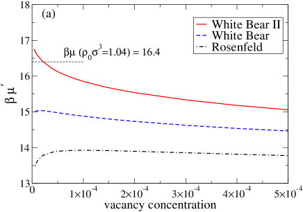
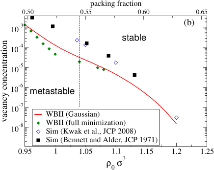
Figure 2: (a): The constrained chemical potential $\mu^{\prime}(\rho_{0},n_{\rm vac})$ as obtained by full minimization of the three DFT models at the bulk density $\rho_{0}\sigma^{3}=1.04$. The dashed line shows the value for the chemical potential following from the thermodynamic definition of $\mu=df_{\rm cr}/d\rho_{0}$ where $f_{\rm cr}$ is the free energy density. It is equal for the three DFT models to the given accuracy. If and only if $\mu^{\prime}(\rho_{0},n_{\rm vac})=\mu$, the free energy per particle is minimal and thus thermodynamic consistency holds. (b): Equilibrium vacancy concentration vs. bulk density as obtained for the WBII functional (full line–Gaussian approximation, filled diamonds–full minimization) and compared to available simulation results (open diamonds–Ref. Kwa08 , filled squares–Ref. Ben71 ).

In Sec. III.2 we have derived an expression for the constrained chemical potential $\mu^{\prime}(\rho_{0},n_{\rm vac})$ (see Eq. (30)). Furthermore we recall that $\mu^{\prime}(\rho_{0},n_{\rm vac})$ is precisely the Lagrange multiplier in the constrained minimization of the unit cell free energy, see Eq. (20). We have examined its dependence on $n_{\rm vac}$ and the bulk density $\rho$ for the three functionals with the surprising result that only in the case of the White Bear II functional $\mu^{\prime}(\rho_{0},n_{\rm vac})$ shows a weakly divergent behavior as $n_{\rm vac}\to 0$. The divergence appears to be weaker than $-\ln n_{\rm vac}$, however. Furthermore only for the White Bear II functional the consistency condition (21) is fulfilled for a (small and) finite equilibrium vacancy concentration $n_{\rm vac,0}$. There is no minimum for the free energy per particle $F/N$ upon variation of $n_{\rm vac}$ for the cases of the Rosenfeld and the White Bear functional (neither in the Gaussian approximation nor for full minimization). This is consistent with Tarazona’s finding of no minimum for $n_{\rm vac}>10^{-8}$ using the Gaussian approximation in the Rosenfeld functional Tar00 . As an exemplary result, we show $\mu^{\prime}(\rho_{0},n_{\rm vac})$ for $\rho_{0}\sigma^{3}=1.04$ (coexistence) for the three functionals, see Fig. 2 (a). The large discrepancies between results for the three functionals is somewhat surprising, given the fact that $F/N$ varies only very little (in the Gaussian approximation we have $\beta F/N=4.929$ [RF], 4.912 [WB], 4.970 [WBII] at this density). Our results for the explicit minimization also question the reliability of the approach taken in Ref. Gro00 to calculate $n_{\rm vac,0}$. It appears that the equilibrium vacancy concentrations and corresponding free energy minima are artefacts of the approximations used therein (isotropic density distributions around lattice sites and an expansion around the close–packing limit).

In Fig. 2 (b) we show the variation of the equilibrium vacancy concentration with the bulk density for the WBII functional. There is reasonable agreement between the Gaussian approximation and the full minimization. However, the predicted $n_{\rm vac,0}$ is consistently smaller (up to one order of magnitude) than available simulation results. Nevertheless one should keep in mind that the DFT results do not follow from an explicit computation of the free energy of a vacancy $f_{\rm vac}$ (see Eq. (24)) as the simulations do. It would be interesting in the future to calculate $f_{\rm vac}$ through an explicit minimization of DFT around a fixed vacancy. Note that an initial attempt in that direction has been undertaken in Ref. Sin05 using the MWDA.

An important implication arises from the fact that the consistency condition (21), $\mu^{\prime}(\rho_{0},n_{\rm vac,0})=df_{\rm cr}/d\rho_{0}$, can be fulfilled only for the WBII functional. It means that a free DFT minimization of the fluid–crystal interface which is consistent with the coexistence data from the Maxwell construction (see Tab. 2) will not be possible with the WB and the RF functionals. This follows since the fluid chemical potential at coexistence does not match the crystal chemical potential obtained by full mimimization.

V.3 Density distributions

The density distribution in the hard sphere crystal consists of nearly isolated density peaks around the lattice sites,

$$\rho_{\rm cr}(\mathbf{r})=\sum_{{\rm lattice\;sites}\;i}\rho(\mathbf{r}-\mathbf{r}_{i})$$ (40)

with no appreciable overlap in the tails of $\rho(\mathbf{r})$. In first approximation, $\rho(\mathbf{r})$ is a Gaussian with a width parameter $\alpha$,

$$\rho(\mathbf{r})\approx\rho_{\rm G}(r)=\left(\frac{\alpha}{\pi}\right)^{\frac{3}{2}}\exp(-\alpha r^{2})\;.$$ (41)

We will analyze the deviations from the Gaussian form in terms of an average radial deviation $f_{\Delta{\rm G}}(r)$ and an anisotropic deviation $f_{\rm aniso}(\mathbf{r})$:

$$\rho(\mathbf{r})\approx\rho_{\rm G}(r)\;f_{\Delta{\rm G}}(r)\;f_{\rm aniso}(\mathbf{r})\;.$$ (42)

The average radial deviation will be parametrized as

$$f_{\Delta{\rm G}}(r)=\exp\left[b_{2}\,\alpha r^{2}+b_{4}(\alpha r^{2})^{2}+b_{6}(\alpha r^{2})^{3}\right]\;,$$ (43)

where $b_{2},b_{4},b_{6}\ll 1$ are expected to be small. For the analysis of the directional anisotropy we apply a polynomial expansion in the form:

$$f_{\rm aniso}(\mathbf{r}) = 1+K_{4}\,\alpha^{2}\,\left(x^{4}+y^{4}+z^{4}-\frac{3}{5}r^{4}\right)+K_{6}\,\alpha^{3}\,\left(x^{6}+y^{6}+z^{6}-\frac{3}{7}r^{6}\right)\;.$$ (44)

This corresponds to the leading two terms in the cubic cell asymmetry (consistent with the point symmetry of the fcc lattice).

V.3.1 Gaussian width parameter

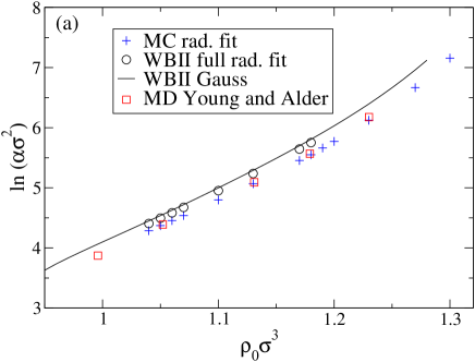
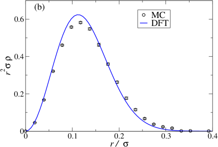
Figure 3: (a): Logarithm of the Gaussian width parameter $\alpha$ vs. bulk density $\rho_{0}$: DFT–WBII in Gaussian approximation (full line), DFT–WBII in full minimization (circles), extrapolation to the thermodynamic limit in MC ($+$ symbols) and results from Ref. You74 (squares). (b): radial probability $r^{2}\rho(r)$ in [100] direction for the bulk density $\rho_{0}\sigma^{3}=1.04$. Comparison between DFT and our simulations.

For the DFT results, the width parameter $\alpha$ is the only minimization parameter in the Gaussian approximation once the normalization is fixed. From the results of the full minimization we determined $\alpha$ by a global fit with the Gaussian form (41) to the lattice peak density distribution. The same was done using the MC data, additionally the value $\alpha_{\infty}$ in the thermodynamic limit was determined by the extrapolation from the values at finite box length $L$ through the relation $\alpha_{N}=A/N^{1/3}+\alpha_{\infty}$ You74 . For the densities $\rho_{0}\sigma^{3}=1.05$ and 1.13 we checked and confirmed this scaling for the four values $N=2916$, 5324, 8788 and 13500. For the other bulk density values, we used $N=5324$ and 13500 to determine $\alpha_{\infty}$.

In Fig. 3 (a) we compare the DFT results for $\alpha$ with $\alpha_{\infty}$ from our MC simulations and a corresponding width parameter extracted from the work of Young and Alder You74 . There the mean square deviation was determined which we converted to the Gaussian width parameter by assuming the Gaussian form for $\rho(\mathbf{r})$: $\alpha=3/(2\langle r^{2}\rangle)$. There is excellent agreement between the two simulations and also fair agreement between DFT and simulations. The Gaussian peaks in DFT are narrower than the simulated peaks which is similar to (M)WDA results although in (M)WDA the quantitative deviation is already considerable (compare e.g. with Tab. I in Ref. Tej95 ). The radial probability, proportional to $r^{2}\rho(r)$, along the $[100]$ direction is shown in Fig. 3 (b). As a remark, earlier MC data for the radial probability were erroneously scaled in the graphical presentations of Ref. Ohn93 .

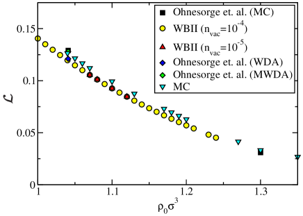
Figure 4: Lindemann parameter ${\cal L}$ vs. bulk density $\rho_{0}$ for Monte Carlo simulation (MC) and DFT, also in comparison with Ref. Ohn93 (Ohnesorge et. al.). Data for (M)WDA from Ref. Ohn93 are taken for full minimization.

In order to quantify the spread of the density distribution around a solid peak it is convenient to define the Lindemann parameter Lin10 ; Ubb78 as the dimensionless root mean-square displacement:

$${\cal L}=\frac{1}{r_{nn}}\sqrt{\int_{WSC}d^{3}rr^{2}\rho(\mathbf{r})}\;.$$ (45)

Here the spatial integration is over a Wigner-Seitz cell ($WSC$) centered around a lattice position at the origin and $r_{nn}=\sigma\left(\sqrt{2}/\rho_{0}\right)^{1/3}$ denotes the distance between two nearest neighbours in the crystal lattice. Data for the Lindemann parameter ${\cal L}$ versus bulk density $\rho_{0}$ are shown in Fig. 4. Clearly, $\cal L$ is about $0.13$ at melting and decreases with increasing density. The Monte Carlo data published earlier in Ref. Ohn93 agree with those from our simulations. All density functionals considered here (WDA, MWDA, WBII) yield Lindemann parameters which are only slightly lower than the simulation data. However, the density profiles from (M)WDA and WBII differ, the agreement in the value of ${\cal L}$ is due to an unphysical high interstitial density in the (M)WDA profiles Ohn93 .

V.3.2 Deviations from the Gaussian form and anisotropy

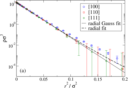
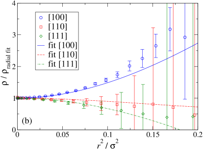
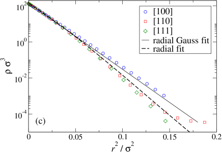
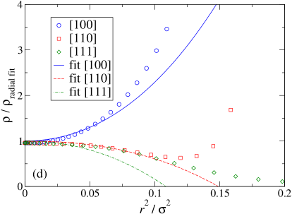
Figure 5: Lattice site density distributions along the lattice directions [100], [110] and [111] for the bulk density $\rho_{0}\sigma^{3}=1.04$. Panels (a) and (b) show MC results ($N=8788$), panels (c) and (d) results from DFT–WBII. Panels (a) and (c) show $\rho$ vs. $r^{2}$ in logarithmic scale, thus illustrating the deviation from a Gaussian form (straight line). The full line here is a fit to the Gaussian form $\rho_{\rm G}$ (Eq. (41)) with the parameter $\alpha=77.5$ (MC) and $\alpha=84.4$ (DFT–WBII). The dashed line is a fit to the non–Gaussian form $\rho_{\rm G}\,f_{\Delta{\rm G}}$ (see Eq. (43)) with the parameters $b_{2}=-0.011$, $b_{4}=0.0021$, $b_{6}=-0.0002$ (MC) and $b_{2}=0.090$, $b_{4}=-0.029$, $b_{6}=0.0009$ (DFT–WBII). Panels (b) and (d) show the density along the three lattice directions divided by $\rho_{\rm G}\,f_{\Delta{\rm G}}$. The lines show the corresponding anisotropies along the three lattice directions resulting from a fit to $f_{\rm aniso}$ (see Eq. (44)) with the parameter $K_{4}=0.022$ (MC) and $K_{4}=0.039$ (DFT–WBII).

In Figs. 5 and 6 we show in an exemplary way the density distributions in the principal lattice directions [100], [110] and [111] for the densities $\rho_{0}\sigma^{3}=1.04$ (near coexistence) and $\rho_{0}\sigma^{3}=1.20$, respectively. The simulation data are always very close to the Gaussian form with the coefficient $b_{4}$ of the leading deviation from the Gaussian form being small, $|b_{4}|\lesssim 0.01$ (see panel (a) in Figs. 5 and 6). Interestingly, $b_{4}$ changes sign at around $\rho_{0}\sigma^{3}=1.10$, indicating that below that density the distribution is wider than a Gaussian (larger curtosis) and above that density the distribution is narrower than a Gaussian (smaller curtosis). In DFT–WBII the density distribution has a smaller curtosis than a Gaussian with $b_{4}\approx-0.03$ for the range of densities 1.04 to 1.20 (see panel (c) in Figs. 5 and 6). Turning to the asymmetries we note that our ansatz (Eq. (44)) describes the data for small distances $r$ very well and starts to deviate only when the overall density has dropped by a factor $10^{4}$ compared to the center of the peak. This is illustrated in panels (b) and (d) in Figs. 5 and 6 where we compare the fit to the anisotropic part $f_{\rm aniso}$ to the quotient of the density profile with the purely radial fit, $\rho(\mathbf{r})/(\rho_{\rm G}(r)\;f_{\Delta{\rm G}}(r)\;)$ (see Eq. (42)). The qualitative behavior of the density distribution in the principal lattice directions is the same for MC and DFT–WBII, only the magnitude of the leading anisotropy coefficient $K_{4}$ is larger in DFT–WBII by about a factor 1.7. The agreement in sign and order of magnitude in $K_{4}$ with simulations distinguishes fundamental measure theory from the (M)WDA approach where an opposite sign is obtained Ohn93 . (Intuitively, the density distribution in [110] direction should be narrower than in [100] since in [110] direction the next neighbor is closer.)

In Fig. 7 we show the value of $K_{4}$ for a range of bulk densities from the fits to both MC and DFT–WBII results. The scatter in the data is a result of the uncertainty in the fits, but one can clearly observe a trend to lower $K_{4}$ for higher density. This would be consistent with the observation in Ref. You74 that towards close–packing the density distribution becomes Gaussian ($K_{4}=0$). We note furthermore that we could not extract any meaningful results for the next–to–leading anisotropy coefficient $K_{6}$ whose modulus appears to be smaller than $|K_{4}|$ but the error estimate is always of about the same magnitude. Finally, we remark that our results for $K_{4}$ are in quantitative agreement to earlier computer simulation data published in Ref. Ohn93 .

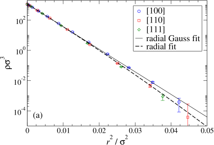
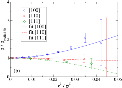
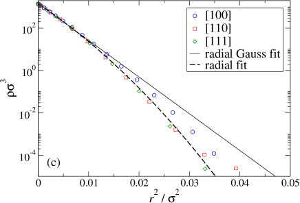
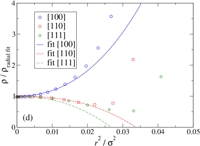
Figure 6: Lattice site density distributions along the lattice directions [100], [110] and [111] for the bulk density $\rho_{0}\sigma^{3}=1.20$. Panels (a) and (b) show MC results ($N=8788$), panels (c) and (d) results from DFT–WBII. Panels (a) and (c) show $\rho$ vs. $r^{2}$ in logarithmic scale, thus illustrating the deviation from a Gaussian form (straight line). The full line here is a fit to the Gaussian form $\rho_{\rm G}$ (Eq. (41)) with the parameter $\alpha=343.7$ (MC) and $\alpha=399.0$ (DFT–WBII). The dashed line is a fit to the non–Gaussian form $\rho_{\rm G}\,f_{\Delta{\rm G}}$ (see Eq. (43)) with the parameters $b_{2}=0.014$, $b_{4}=-0.0054$, $b_{6}=-0.00002$ (MC) and $b_{2}=0.075$, $b_{4}=-0.026$, $b_{6}=-0.0002$ (DFT–WBII). Panels (b) and (d) show the density along the three lattice directions divided by $\rho_{\rm G}\,f_{\Delta{\rm G}}$. The lines show the corresponding anisotropies along the three lattice directions resulting from a fit to $f_{\rm aniso}$ (see Eq. (44)) with the parameter $K_{4}=0.014$ (MC) and $K_{4}=0.025$ (DFT–WBII).

VI Discussion and Conclusion

In this work we have performed a comparative study of the free energies and the density distributions in hard sphere crystals using Monte Carlo simulations and density functional theory (employing Fundamental Measure functionals). Using a recently introduced simulation technique, we could obtain crystal free energies to a high precision (see Tab. 1) which are consistent with the most recent parametrizations of empirical equations of state and allowed us to determine the crystal free energy in the close–packing limit with a higher accuracy than before (see Eq. (39)). The free energies from Fundamental Measure theory are also in good agreement with the simulation results and demonstrate the applicability of these functionals to the treatment of other problems involving crystallization. The agreement between FMT and simulations on the level of the free energies is also reflected in the density distributions around single lattice sites (see Figs. 5 and 6). Overall, the peak widths and anisotropy signs for different lattice directions agree, it is found that FMT gives slightly narrower peaks with more anisotropy than seen in the simulations.

The deviations we observe between simulation and FMT point to possibilities of further improvement in the FMT functionals. Tarazona’s construction of the tensor part of these functionals is an approximate representation of the three–cavity overlap situation (see Fig. 1) which leads to a complicated expression. It would be interesting to study the close–packing limit of this expression in a systematic manner.

Additionally we studied theoretically for the constrained minimization in the unit cell (with particle number fixed) the relation of the respective constrained chemical potential $\mu^{\prime}$ to Widom’s trick in a system with fixed vacancy concentration $n_{\rm vac}$. The latter analysis gives a simple relation, $\mu^{\prime}={\rm const.}-\ln n_{\rm vac}$ (see Eq. (30)), which poses a consistency condition on the corresponding FMT results for $\mu^{\prime}$. It turns out that from the three studied variants of FMT, only the White Bear II functional shows the qualitatively correct behavior whereas the Rosenfeld and the White Bear functional give qualitatively incorrect results (see Fig. 2). This implies that for further studies such as the free minimization of the crystal–fluid interface or nucleation processes only the White Bear II functional is a promising candidate.

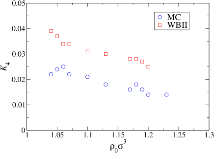
Figure 7: Leading anisotropy coefficient $K_{4}$ vs. bulk density $\rho_{0}$ as obtained from a fit to the density distributions from MC simulations (circles) and from DFT–WBII (squares).

- (1) W. W. Wood and J. D. Jacobson, J. Chem. Phys. 27, 1207 (1957).
- (2) B. J. Alder and T. E. Wainwright, J. Chem. Phys. 27, 1208 (1957).
- (3) P. N. Pusey and W. van Megen, Nature 320, 340 (1986).
- (4) G. Bryant, S. R. Williams, L. Qian, I. K. Snook, E. Perez, and F. Pincet, Phys. Rev. E 66, 060501(R) 2002.
- (5) M. Siebenbürger, M. Fuchs, H. Winter, and M. Ballauff, J. Rheol. 53, 707 (2009).
- (6) U. Gasser, E. R. Weeks, A. Schofield, P. N. Pusey, and D. A. Weitz, Science 292, 258 (2001).
- (7) E. R. Weeks and D. A. Weitz, Phys. Rev. Lett. 89, 095704 (2002).
- (8) H. J. Schöpe, G. Bryant, and W. van Megen, Phys. Rev. Lett. 96, 175701 (2006).
- (9) E. Zaccarelli, C. Valeriani, E. Sanz, W. C. K. Poon, M. E. Cates, and P. N. Pusey, Phys. Rev. Lett. 103, 135704 (2009)
- (10) T. Schilling, H. J. Schöpe, M. Oettel, G. Opletal, and I. Snook, Phys. Rev. Lett. 105, 025701 (2010).
- (11) H. Emmerich, J. Phys.: Condens. Matter 21, 464103 (2009).
- (12) G. Kahl and H. Löwen, J. Phys.: Condens. Matter 21, 464101 (2009).
- (13) R. Evans, Adv. Phys. 28, 143 (1979)
- (14) P. Tarazona, J. A. Cuesta, and Y. Martinez–Raton, in: A. Mulero (Ed.), Theory and Simulation of Hard-Sphere Fluids and Related Systems, Springer, Berlin (2008), pp. 247–342.
- (15) R. Roth, J. Phys.: Condens. Matter 22, 063102 (2010).
- (16) U. M. B. Marconi and P. Tarazona, J. Chem. Phys. 110, 8032 (1999).
- (17) A. J. Archer and M. Rauscher, J. Phys. A: Math. Gen. 37, 9325 (2004).
- (18) A. J. Archer, J. Chem. Phys. 130, 014509 (2009).
- (19) P. Espanol and H. Löwen, J. Chem. Phys. 131, 244101 (2009).
- (20) M. Rex and H. Löwen, Phys. Rev. Lett. 101, 148302 (2008).
- (21) L. J. D. Frink and A. G. Salinger, J. Comp. Phys. 159, 407 (2000).
- (22) D. Goulding and S. Melchionna, Phys. Rev. E 64, 011403 (2001).
- (23) M. Oettel, H. Hansen–Goos, P. Bryk, and R. Roth, EPL 85, 36003 (2009).
- (24) V. Botan, F. Pesth, T. Schilling, and M. Oettel, Phys. Rev. E 79, 061402 (2009).
- (25) P. Tarazona, Phys. Rev. Lett. 84, 694 (2000).
- (26) T. V. Ramakrishnan and M. Yussouf, Phys. Rev. B 19, 2775 (1979).
- (27) A. D. J. Haymet, J. Phys. Chem. 89, 887 (1985).
- (28) G. L. Jones and U. Mohanty, Mol. Phys. 54, 1241 (1985).
- (29) P. Tarazona, Mol. Phys. 52, 81 (1984).
- (30) P. Tarazona, Phys. Rev. A 31, 2672 (1985).
- (31) W. A. Curtin and N. W. Ashcroft, Phys. Rev. A 32, 2909 (1985).
- (32) A. R. Denton, N. W. Ashcroft, and W. A. Curtin, Phys. Rev. E 51, 65 (1995).
- (33) R. Ohnesorge, H. Löwen, and H. Wagner, Europhys. Lett. 22, 245 (1993).
- (34) R. Ohnesorge, H. Löwen, and H. Wagner, Phys. Rev. A 43, 2870 (1991).
- (35) W. A. Curtin and K. Runge, Phys. Rev. A 35, 4755 (1987).
- (36) R. Ohnesorge, H. Löwen, and H. Wagner, Phys. Rev. E 50, 4801 (1994).
- (37) Y. Rosenfeld, Phys. Rev. Lett. 63, 980 (1989).
- (38) R. Roth, R. Evans, A. Lang, and G. Kahl, J. Phys.: Condens. Matter 14, 12063 (2002).
- (39) Y.-X. Yu and J. Wu, J. Chem. Phys. 117, 10156 (2002).
- (40) H. Hansen–Goos and R. Roth, J. Phys.: Condens. Matter 18, 8413 (2006).
- (41) Y. Rosenfeld, M. Schmidt, H. Löwen, and P. Tarazona, Phys. Rev. E 55, 4245 (1997).
- (42) J. K. Percus, J. Stat. Mech. 15, 505 (1976).
- (43) P. Tarazona and Y. Rosenfeld, Phys. Rev. E(R) 55, 4873 (1997).
- (44) P.-M. König, R. Roth R. and K. Mecke, Phys. Rev. Lett. 93, 160601 (2004).
- (45) C. H. Bennett and B. J. Alder, J. Chem. Phys 54, 4796 (1971).
- (46) S. Pronk and D. Frenkel, J. Phys. Chem. B 105, 6722 (2001).
- (47) S. K. Kwak, Y. Cahyana, and J. K. Singh, J. Chem. Phys 128, 134514 (2008).
- (48) D. A. Young and B. J. Alder, J. Chem. Phys 60, 1254 (1974).
- (49) B. Groh, Phys. Rev. E 61, 5218 (2000).
- (50) J. F. Lutsko, Phys. Rev. E 74, 021121 (2006).
- (51) V. B. Warshavsky and X. Song, Phys. Rev. E 73, 031110 (2006).
- (52) V. B. Warshavsky and X. Song, J. Chem. Phys. 129, 034506 (2008).
- (53) D. Frenkel and A. Ladd, J. Chem. Phys 81, 3188 (1984).
- (54) C. Vega and E. Noya, J. Chem. Phys 127, 154113 (2007).
- (55) T. Schilling and F. Schmid, J. Chem. Phys 131, 231102 (2009).
- (56) R. J. Speedy, J. Phys.: Condens. Matter 10, 4387 (1998).
- (57) N. G. Almarza, J. Chem. Phys 130, 184106 (2009).
- (58) T. Zykova-Timan, J. Horbach, and K. Binder, J. Chem. Phys. 133, 014705 (2010).
- (59) B. Groh, Phys. Rev. E 61, 3811 (2000).
- (60) D. A. Young and B. J. Alder, J. Chem. Phys 49, 3688 (1968).
- (61) S. P. Singh, C. Kaur, and S. P. Das, Phys. Rev. E 72, 021603 (2005).
- (62) C. F. Tejero, M. S. Ripoll, and A. Perez, Phys. Rev. E 52, 3632 (1995).
- (63) F. A. Lindemann, Phys. Z. 11, 609 (1910).
- (64) A. R. Ubbelohde, The molten state of matter, Chichester, John Wiley, 1978.