Imaging Spectropolarimetry with IBIS II:
on the fine structure of G-band bright features

Abstract

We present new results from first observations of the quiet solar photosphere performed through the Interferometric BIdimensional Spectrometer (IBIS) in spectropolarimetric mode. IBIS allowed us to measure the four Stokes parameters in the Fe I 630.15 nm and Fe I 630.25 nm lines with high spatial and spectral resolutions for $53$ minutes; the polarimetric sensitivity achieved by the instrument is $3\times 10^{-3}$ the continuum intensity level.

We focus on the correlation which emerges between G-band bright feature brightness and magnetic filling factor of $\sim 10^{3}$ G (kG) fields derived by inverting Stokes $I$ and $V$ profiles. More in detail, we present the correlation first in a pixel-by-pixel study of a $\simeq 3$ arcsec wide bright feature (a small network patch) and then we show that such a result can be extended to all the bright features found in the dataset at any instant of the time sequence. The higher the kG filling factor associated to a feature the higher the brightness of the feature itself. Filling factors up to $\simeq 35$% are obtained for the brightest features. Considering the values of the filling factors derived from the inversion analysis of spectropolarimetric data and the brightness variation observed in G-band data we put forward an upper limit for the smallest scale over which magnetic flux concentrations in intergranular lanes produce a G-band brightness enhancement ($\simeq 0.1^{\prime\prime}$). Moreover, the brightness saturation observed for feature sizes comparable to the resolution of the observations is compatible with large G-band bright features being clusters of sub-arcsecond bright points. This conclusion deserves to be confirmed by forthcoming spectropolarimetric observations at higher spatial resolution.

1. Introduction

Solar magnetic fields manifest in the photosphere in a large variety of structures. At sub-arcsecond spatial scales they can appear concentrated in bright and roundish features, located in convective downflow regions, preferentially at the vertexes of granules. These bright features, first observed by Dunn & Zirker (1973) and Mehltretter (1974) in the network, are ubiquitous on the solar photosphere (Sánchez Almeida et al. 2004; de Wijn et al. 2005; Bovelet & Wiehr 2008; Sánchez Almeida et al. 2010) and their aggregation in active regions form, on larger spatial scales, faculae (e.g., Frazier & Stenflo 1972; Mehltretter 1974; Rabin 1992). Their photometric properties are largely dependent on the spectral range in which they are observed (e.g., Sütterlin et al. 1999; Langhans et al. 2004; Tritschler & Uitenbroek 2006; Beck et al. 2007). In particular, they show enhanced contrast with respect to the quiet Sun average intensity (typically $30$%) when observed in the G-band (around $430.8$ nm) and are therefore referred to as G-band bright points (Muller & Roudier 1984). Due to their small size, the investigation of these features has been long hampered by spatial resolution limits imposed by instrumentation and atmospheric seeing. During the last decade, the development of Adaptive Optic Systems as well as post-facto restoration techniques (Löfdahl et al. 1998; Löfdahl 2002; van Noort et al. 2005) has allowed studies that focused on the photometric (e.g., Keller 1992; Berger et al. 1995; Berger & Title 1996, 2001; Berger et al. 2004; Bovelet & Wiehr 2003; Berger et al. 2007; Utz et al. 2009a; Kobel et al. 2009), dynamic (e.g., Bovelet & Wiehr 2003; Nisenson et al. 2003; de Wijn et al. 2005; Ishikawa et al. 2007; Langangen et al. 2007; de Wijn et al. 2008; Utz et al. 2009b) and magnetic (e.g., Muller et al. 2000; Berger & Title 2001; Berger et al. 2007; Ishikawa et al. 2007; Bharti et al. 2006; Beck et al. 2007; de Wijn et al. 2008; Viticchié et al. 2009) properties of these small-size magnetic flux concentrations. In particular, observations have revealed that these are highly structured. Berger et al. (2004) reported that in active regions, at locations of high magnetic flux density correspond in both Ca and G-band images a large variety of features that they describe as filamentary crinkles-like structures, roundish flower- and ribbon-like features and, at the smallest spatial scales, point-like brightenings. Photometric properties and magnetic flux density are not constant within most of them, both contrast and magnetic flux density being in general higher at their edges and lower at their centers. The opposite is observed for point-like features. All these structures are highly dynamic and can evolve one into another (Rouppe van der Voort et al. 2005; Viticchié et al. 2009). In quiet Sun regions, most of the features are point-like and are often clustered in groups or “patches” at the edges of granules and mesogranules (Sánchez Almeida et al. 2004; de Wijn et al. 2005, 2008). The properties of G-band bright features (e.g., dimension and contrast) strongly depend on the angular resolution of observations so that it is hard to rigorously define the “real bright point”. For this reason, in the following we will use the name “bright feature” to indicate a local excess of brightening in the intergranular lanes of G-band filtergrams, independently of the properties of the feature itself.

Theoretically, bright features were investigated through the model of flux-tube (Spruit 1976), a small-size concentration of magnetic field surrounded by field-free plasma. Due to the high magnetic pressure inside the kG flux tube, the gas pressure (gas density) is strongly reduced causing the photons to escape from deep photospheric layers that are hotter than the surrounding plasma in cold intergranular lanes. Numerical static and dynamic models of isolated (Deinzer et al. 1984; Knoelker et al. 1988; Pizzo et al. 1993; Steiner et al. 2001; Steiner 2005) or clustered (Caccin & Severino 1979; Okunev & Kneer 2005; Criscuoli & Rast 2009) flux tubes, have proved to be successful in reproducing many of the observed properties, such as the enhancement of contrast toward the limb and in some molecular bands (in particular CH and CN bands, e.g., Schüssler et al. 2003), the presence of dark lanes which often accompany the bright features in off-disk center observations, and the suppression of convective motions within them.

From the above figure follows that G-band bright features are proxies for kG fields in the solar photosphere. On the other hand, the inspection of movies reveals that the brightness of the features is not constant with time but intermittently can vary such that features can appear dark or bright at different instant. This evidence questions the flux tube evacuation as the principal physical mechanism responsible for contrast enhancement in small size magnetic concentrations.

The understanding of the relation between the contrast measured in molecular bands and the properties of magnetic concentrations is of relevance for all those studies which employ broad-band imaging as proxy of strong magnetic fields (de Wijn et al. 2005). In particular G-band imaging of the solar photosphere, thanks to the high spatial resolution that can be achieved in these data, is an independent and complementary tool to spectropolarimetric observations. This is of great relevance, for instance, for the investigation of the presence of kG fields in the quiet Sun, which is still a debated topic in solar physics (see de Wijn et al. 2009, for a review).

In Viticchié et al. (2009) the first results from observations performed with IBIS (Cavallini 2006) in spectropolarimetric mode revealed the advantages of combining high spatial resolution spectropolarimetry simultaneous and co-spatial to G-band imaging in the study of the temporal evolution of bright features in the quiet Sun. In the present work we report further results obtained from the same analysis concerning the relation between magnetic filling factor and brightness of G-band bright features. More in detail, these complete and corroborate the picture outlined in Viticchié et al. (2009) only for three peculiar cases. The aim of this paper is to go more into the details of the capabilities of IBIS and to confirm the finding of the relation between kG magnetic filling factor and G-band bright feature intensity by exploiting the whole analyzed dataset. Such a relation will eventually allow us to conclude on the fine structuring of G-band bright features.

In § 2 the dataset is presented, in § 3 the adopted analysis methods are described, in § 4 we report the results from the analysis that are then discussed in § 5; in § 6 the main conclusions are summarized.

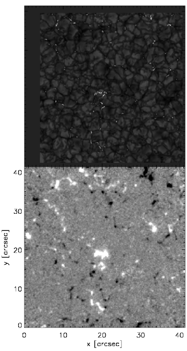
Figure 1.— Two snapshots from the analyzed dataset. Upper panel: G-band snapshot; bright feature intensity has been enhanced to show the result of the automatic identification procedure. Lower panel: COG magnetogram saturated at $\pm 200$ G. The images refer to 16:42:29 UT.

2. Data

A quiet region at disk center was observed on November 21, 2006 from 16:24 UT to 17:17 UT with IBIS, at the NSO/Dunn Solar Telescope. The field-of-view (FOV) was approximatively $40^{\prime\prime}\times 40^{\prime\prime}$. The acquired dataset consists of $50$ scans of the two Fe I $630$ nm lines performed with a cadence of $89$ seconds. The seeing during the acquisition of the first $36$ scans (which have been analyzed in this work) was excellent and stable allowing the Adaptive Optics system (Rimmele 2004) to achieve near diffraction-limited performance. The lines were sampled at $45$ wavelength points with a spectral FWHM of $2$ pm and a step of $2.3$ pm. In the scanning procedure the telluric line in between the two Fe I lines was skipped while the O₂ 630.28 nm one was sampled with three points; this line allows us to set the absolute wavelength scale of our spectropolarimetry measurements.

To perform spectropolarimetric measurements, the incoming light to IBIS is modulated by a pair of nematic liquid crystal variable retarders placed in a collimated beam in front of the field stop of the instrument. The light is analyzed by a beam splitter in front of the detector, imaging two orthogonal states onto the same chip thus allowing for dual-beam spectropolarimetry. The modulation is in such a way that at each wavelength position six modulation states $I+S$ (and its orthogonal states $I-S$) are detected with the following temporal scheme: $S=[+V,-V,+Q,-Q,+U,-U]$. Spectropolarimetric images have a pixel scale of $0.18^{\prime\prime}$. Simultaneous to narrow-band spectropolarimetric data, broad-band ($633.32\pm 5$ nm) counterparts of the same FOV were acquired. The exposure time for both narrow-band and broad-band data is $80$ ms. The pixel scale of broad band data is $0.09^{\prime\prime}$. These reference images are normally used to register their spectropolarimetric counterparts. In this particular observation setup, a post processing Multi-Frame Blind Deconvolution procedure (MFBD; Löfdahl 2002) has been applied to these broad-band images to obtain a master frame from each scan with much reduced seeing degradation and a homogeneous resolution in the whole FOV. We are then able to correct for anisoplanatism applying a de-stretch process on the single broad-band images, using this master frame as reference image. The computed de-stretch matrixes are successively applied also to the spectropolarimetric images.

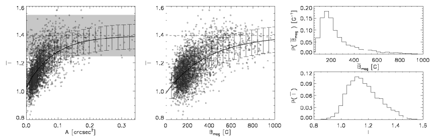
Figure 2.— Average properties of bright features from both G-band images and COG magnetograms. The plots are derived by calculating: the average flux density $\bar{B}_{mag}$, the average G-band intensity $\bar{I}$ (normalized to the average intensity of the time sequence), and the total area $A$ of bright features identified through the automatic procedure described in § 3. In the left panel: $\bar{I}$ vs. $A$ scatter plot. In the central panel: $\bar{I}$ vs. $\bar{B}_{mag}$ scatter plot. In both the plots an exponential fit of the data is reported (solid line). The error bars represent the average standard deviation error of the fit; the horizontal dashed line represent the saturation value $\bar{I}_{sat}$; the shaded area in the left panel represent the standard deviation error of $\bar{I}_{sat}$. For details on the fit procedure refer to § 4.1 and Table 1. In the right panels: histogram for $\bar{I}$ (upper panel) and $\bar{B}_{mag}$ (lower panel), respectively.

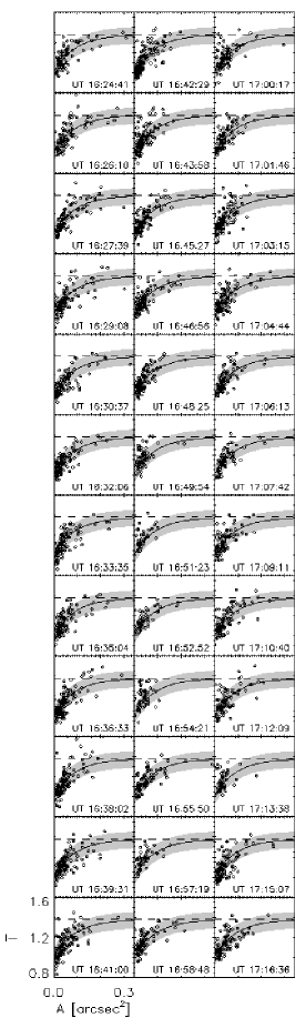
Figure 3.— $\bar{I}$ vs. $A$ scatter plots along the whole acquired time sequence; $\bar{I}$ is normalized to the average G-band intensity of each frame. The time sequence is divided in three columns representing three subsequent time intervals; in each column the time rolls from up to down. Each scatter plot relates $\bar{I}$ and $A$ for each instant of the time sequence. In all the plots the result of the exponential fit shown in the left panel of Fig. 2 is reported (solid line). The shaded area here represents the average standard deviation with respect to the exponential fit (error bars in Fig. 2). The horizontal dashed line represents the saturation value $\bar{I}_{sat}$.

Table 1results from the exponential fits

scatter plot	$a$	$b$	$c$
$\bar{I}$ vs. $A$	$-0.37\pm 0.13$	$-14\pm 7$ [arcsec-2]	$1.4\pm 0.1$
$\bar{I}$ vs. $\bar{B}_{mag}$	$-0.40\pm 0.07$	$-3.0\pm 0.9$ [$10^{-3}$ G-1]	-
$\bar{I}$ vs. $\bar{f}$	$-0.37\pm 0.04$	$-7.0\pm 0.9$	-

Due to the classical mounting of the double etalon system, the spectral bandpass of IBIS experiences a wavelength-dependent blueshift within the FOV. For each pixel in the FOV, the blueshift amount is computed fitting a template line profile on the calibration dataset of flat-fields acquired just after the observations, taking into consideration also the displacements introduced by the de-stretch procedure. The calibration data includes flats, darks, resolution targets, grids for alignment and instrumental polarization calibration measurements. The IBIS spectropolarimetric $I\pm S$ images were then reduced applying the pipeline developed at NSO and slightly modified for this dataset needs, which takes care of dark subtraction, pixelwise gain calibration, co-alignment with broad-band images, blueshift correction, de-stretching and also the co-registration of all images in each scan and for the whole dataset. The frames were then combined and corrected for instrumental polarization to retrieve the Stokes vectors. At this stage, also the telescope induced polarization is taken into account (as in Judge et al. 2010). We used the closest DST telescope calibration, which was measured on February 16, 2007.

Additionally to broad-band and narrow-band data, G-band filtergrams ($430.5\pm 0.5$ nm) were acquired for a slightly smaller FOV; the pixel scale of such filtergrams is $0.037^{\prime\prime}$, while the exposure time is $15$ ms. The fine alignment between G-band and broad-band images was performed through grid line targets. Tracking inaccuracies were corrected via a correlation procedure. A post processing MFBD procedure was applied also to the G-band images.

As already stated, the quality of spectropolarimetric data has been improved by applying on each spectropolarimetric image the same shifts necessary to align and destretch the associated broad-band image with respect to the MFBD restored broadband image. In this way, the seeing-induced crosstalk is reduced and a spatial resolution comparable with that of the individual narrow band images is reached. The angular resolution of the spectropolarimetric dataset has been estimated to be $0.4^{\prime\prime}\simeq 2$ pixels.

The average noise level for Stokes $V$, measured as standard deviation of the circular polarization in continuum wavelengths, is $\sigma_{V}=3\cdot 10^{-3}I_{C}$ (here $I_{C}$ is the continuum intensity).

3. Data analysis

Stokes $V$ measurements are exploited in two different ways to conclude on the magnetic properties of G-band bright features. Using the center-of-gravity method (COG, Rees & Semel 1979), we calculate longitudinal magnetic flux density maps; the COG method is not affected by saturation in the kG regime, for this reason it results suitable for the analysis of kG bright features.

Beside the COG approach, the inversion of the Stokes $I$ and $V$ profiles of the two lines with the SIR code (Ruiz Cobo & del Toro Iniesta 1992) allows us to determine the line-of-sight (LOS) field strength and the magnetic filling factor. The polarization profiles emerging from the pixels under examination are interpreted by means of two atmospheric components: one is magnetized while the other is field-free. The portion of each pixel occupied by the magnetized component (i.e., the magnetic filling factor $f$) is a free parameter of the inversion. The temperature stratification of each component is modified with two nodes; as initial guess the Harvard Smithsonian Reference Atmosphere model (Gingerich et al. 1971) is used. The LOS velocities and the field strength in the magnetized component are both assumed to be constant with height. The stray-light contamination is considered to be unpolarized and is defined by averaging the Stokes $I$ spectra in a region of $1$ arcsec around each analyzed pixel. Such a contribution is added to the Stokes $I$ profile synthesized from the model atmosphere weighted by the stray-light factor $\alpha$; the most probable value for the latter factor is $\alpha\simeq 85\%$. No macroturbulence and microturbulence are considered. Finally, the finite spectral resolution of the instrument is taken into account using the known spectral PSF of the instrument (Reardon & Cavallini 2008).

Our analysis is focused on the properties of magnetic bright features. For this reason we analyze exclusively very strong polarization signals, i.e., Stokes $V$ signals above $4\times\sigma_{V}$ in both Fe I lines. In spite of the severe selection rule, a total of about $53000$ pixels are considered; these correspond to approximately $3\%$ of the whole FOV at any step of the time sequence and are found to be in strong correlation with bright features in simultaneous and cospatial G-band frames. On the other hand, linear polarization signals are found to be always below the selection threshold so that no full Stokes inversion is performed. In Beck et al. (2007) the authors were able to perform full Stokes inversions in bright feature locations with a polarimetric sensitivity three times better than ours for the visible lines.

To automatically identify the bright features in G-band filtergrams we adopted the algorithm already used by Sánchez Almeida et al. (2007) for the identification of bright features in $0.2$ arcsec angular resolution G-band images filtergrams acquired at the DOT. The details of the procedure are explained in the paper cited above.

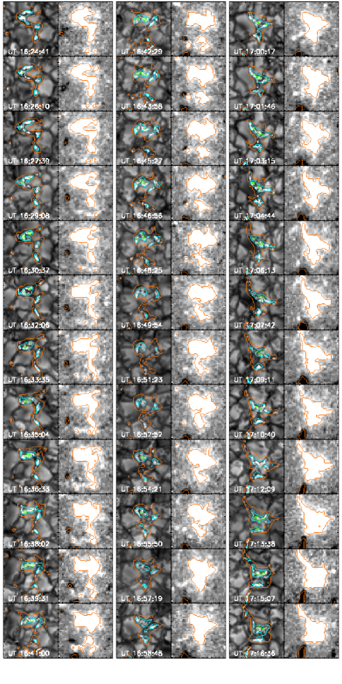
Figure 4.— Magnetic properties of a large bright feature along the whole acquired time sequence. The time sequence is divided in three columns representing three subsequent time intervals; in each column the time rolls from up to down. For each instant of the sequence two frames are reported: a G-band image detail of the bright feature under examination (left frame) and a COG magnetogram saturated to $\pm 200$ G (right frame). The magnetic properties as obtained from the inversion analysis are reported as contours: the kG field region (orange contour), the region with magnetic filling factor $>15\%$ (sky-blue contour), and the region with magnetic filling factor $>30\%$ (green contour). The distance between the major ticks of the frames is of $1.4$ arcsec.

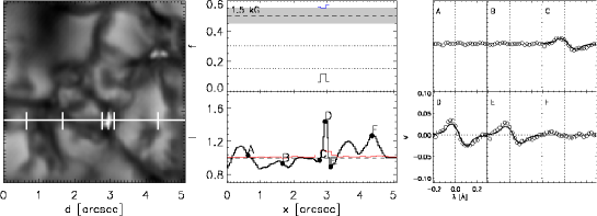
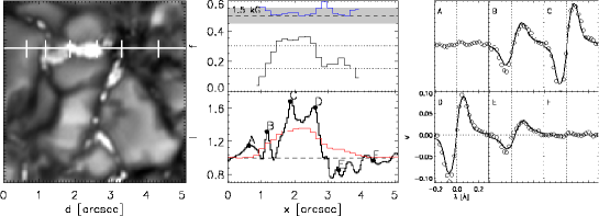
Figure 5.— Two examples of slice profiles from the results of the inversion analysis and G-band intensity images. These are representative of two interesting cases, namely, a $\simeq 0.3$ arcsec wide isolated bright feature observed at 16:42:29 UT (upper panel), and an extended bright feature in a kG magnetized intergranular lane observed at 16:39:31 UT (lower panel, see also Fig.4). Left panel: a $d\times d$ G-band intensity detail image to identify the position of the slice here represented as a white line (left image). Central panel, upper plot: magnetic filling factor $f$ derived from the inversion analysis (solid black line), the horizontal dotted lines represent the levels defining the filling factor contours in Fig. 4 (i.e., $f=15$% and $f=30$% levels, respectively); here we plot also the magnetic field strength derived from the inversion (blue line) whose variation refers to the $1.5$ kG level represented as a dashed line; the shaded area represent a $\pm 150$ G field strength variation around the $1.5$ kG level. Central panel, lower plot: G-band intensity along the slice normalized to the average intensity of the time sequence (black line) and $|V|$ maximum amplitude along the slice (red line) properly rescaled to be compared with the G-band intensity profile. The histogram-like representation adopted in these plots allows us to highlight the different pixel scales of G-band data ($0.037$ arcsec) and spectropolarimetric data ($0.18$ arcsec), respectively. Right panel: Fe I $6301.5$ Å Stokes $V$ profiles from both observation and inversion analysis (right panels, symbols and solid line, respectively) picked at different positions along the slice (named as $A$, $B$, $C$, $D$, $E$, and $F$); each profile is represented in the $x-y$ range specified in the plot $D$ (wavelengths are represented as deviation with respect to the laboratory wavelength of the line). Positions $A$, $B$, $C$, $D$, $E$, and $F$ are reported in the G-band detail image as ticks and on the intensity profile with dots.

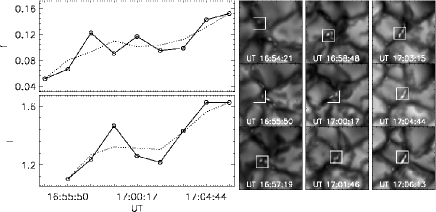
Figure 6.— Temporal variation of both brightness and magnetic filling factor in a process of merging of bright features. Left panel, upper plot: temporal variation of the magnetic filling factor. Left panel, lower plot: temporal variation of bright feature brightness (normalized to the average intensity of the time sequence). In both the plots the dotted line represents the trend of the evolution obtained by smoothing the temporal variation represented with the solid line. In the right panel the time sequence is divided in three columns representing three subsequent time intervals; in each column the time rolls from up to down. Here, G-band image details of the bright feature under examination are reported. The square indicates the region from which the quantities in the left panel are derived; this is placed where the strongest Stokes $V$ signal is found in the region under examination. At UT 16:54:21 no bright features were found by the automatic procedure in the selected square.

4. Results

We investigated the magnetic properties of G-band bright features through both COG magnetograms and inversion of Stokes $V$ profiles. In the following we present the results derived from such analyses in two separated sections. The first one (§ 4.1), concerning the analysis of magnetograms, allows us a straightforward comparison with the results presented in the extended literature on this topic (see § 1). The second one (§ 4.2), concerning the inversion analysis, offers new insight on the relation between photometric and magnetic properties of G-band bright features sheding new light on the results in § 4.1.

4.1. G-band intensity and COG maps

Fig. 1 (upper panel) shows an example of bright features identified through the automatic procedure described in § 3 on one of the snapshots of the sequence. The average fraction of solar photosphere occupied by such features during the time sequence is about $0.6$%. Their linear dimensions range between $\simeq 0.1$ arcsec up to $2-3$ arcsec. They appear in a great variety of shapes: from the point-like (at the angular resolution of the G-band data) to the extended and elongated (e.g., the feature in the center of the FOV in the upper panel of Fig. 1).

In Fig. 2 (left panel) we report the scatter plot relating the average G-band intensity of bright features $\bar{I}$ (normalized to the average intensity of the time sequence) and their area $A$. The apparent linear relation between $\bar{I}$ and $A$ is broken for $A>0.1$ arcsec² and $\bar{I}$ seems to saturate for larger $A$ values. Hence, we fitted an exponential function $a_{1}\cdot e^{b_{1}x}+c_{1}$ on the scatter plot, where $a_{1}$, $b_{1}$, and $c_{1}$ are free parameters of the fit. The exponential fit is overplotted on the data while the derived parameters are reported in Table 1. According to the exponential fit, we can define a saturation level for the average intensity of large bright features approximatively at $c_{1}=\bar{I}_{sat}=1.4$. In the plot $\bar{I}_{sat}$ is represented as a horizontal dashed line, while the shaded area represents the error on $\bar{I}_{sat}$ derived from the fit procedure.

In Fig. 2 (central panel) we report a scatter plot relating the average COG magnetic flux density $\bar{B}_{mag}$ and $\bar{I}$ of identified bright features. In order to compare these quantities, we rescaled the COG magnetograms (Fig. 1 lower panel) at the G-band pixel scale, so that we could associate to each identified feature its $\bar{B}_{mag}$ and $\bar{I}$ computed over the pixels forming the region itself. We find that also the relation between $\bar{B}_{mag}$ and $\bar{I}$ can be described by an exponential law. The fit displayed in Fig. 2 (central panel) was obtained by imposing the saturation level to be $\bar{I}_{sat}$ (i.e., $a_{2}\cdot e^{b_{2}x}+\bar{I}_{sat}$). The values for $a_{2}$ and $b_{2}$ derived from the fit are reported in Table 1.

In the rightmost panels of Fig. 2 we report the histograms for $\bar{B}_{mag}$ and $\bar{I}$. The most probable value for the average flux density in bright features is approximatively $100-150$ G with a tail up to $\simeq 800$ G, while the normalized average intensity ranges between $0.9$ and $1.4$ with the most probable value at $\simeq 1.1$.

Both the scatter plots in Fig. 2 have been defined by considering the data from the whole time sequence. It is important to specify that both plots are good representations of the relations between the magnetic flux density, the G-band intensity, and the area of bright features at any instant of the time sequence. This has been checked by comparing the behavior of all $36$ scatter plots taken individually along the time sequence with the scatter plots of Fig. 2. In Fig. 3 we show one of the results of such a check; we report the $\bar{I}$ vs. $A$ scatter plot for each instant of the time sequence in comparison with the results of the exponential fit in Fig. 2 (left panel). We have to specify that in Fig. 3 $\bar{I}$ is obtained by normalizing the intensity to the average G-band intensity of each frame. The agreement between the scatter plots and the exponential behavior derived from the time-integrated scatter plot in Fig. 2 is more than satisfactory. Once the consistency has been verified, we are allowed to use the time integrated scatter plot, as it provides a more statistically sound representation.

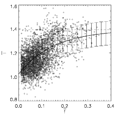
Figure 7.— Correlation between average magnetic filling factor $\bar{f}$ and average G-band intensity $\bar{I}$ (normalized to the average intensity of the time sequence) for bright features in the analyzed dataset. In the plot an exponential fit of the data is reported (solid line). The error bars represent the average standard deviation error of the fit; the horizontal dashed line represent the saturation value $\bar{I}_{sat}$. For details on the fit procedure refer to § 4.1, § 4.2, and Table 1.

4.2. G-band intensity and inversion results

Fig. 4 shows the temporal evolution of the magnetic properties of the largest bright feature in the FOV, as derived from the inversion analysis, together with G-band and COG magnetogram images. The feature can be considered a small network patch, i.e., a region in which the plasma dynamics concentrates kG fields over a region $2-3$ arcsec wide. kG fields are revealed over the entire region comprising the bright feature (orange contour). High magnetic filling factors are found in correspondence with the brightest portions of the feature. Namely, in these regions $f$ is mostly higher than $15$% and can reach values up to $\simeq 35$%. Such values are much higher than typical $f$ values for kG fields in the internetwork which have been measured to be of few percents (e.g., Viticchié et al. 2010). This correlation is persistent along the whole time sequence (cfr., the different snapshots of Fig. 4).

Fig. 5 shows the pixel-by-pixel correlation between Stokes $V$ amplitude, magnetic filling factor $f$, and G-band intensity $I$ (normalized to the average intensity of the whole time sequence) along slices extracted from the analyzed dataset. This representation is similar to the one adopted by Berger et al. (2004) to represent results from observations performed in different bands. Stokes $V$ profiles from both observations and the inversion analysis for selected positions along the slices are also represented in the figure. These profiles are well fitted by the SIR code under the adopted inversion hypotheses (§ 3). In the two panels of the figure the variation of the G-band intensity is found to be in correlation with both Stokes $V$ amplitude and $f$, while the magnetic field strength does not show any correlation with these quantities; in fact, it slightly varies around $1.5$ kG. The two cases reported in Fig. 5 are representative of a point-like bright feature in an intergranular lane (upper panel), and an extended bright feature in an intergranular lane (lower panel).

The upper panel of Fig. 5 displays the different capabilities of G-band and spectropolarimetric data in resolving the properties of bright magnetic features. In fact, the bright feature is found to be $\simeq 0.15$ arcsec wide, i.e., four pixels in G-band data, while the polarization signal is spread over a region of $\simeq 0.7$ arcsec, i.e. four pixel in spectropolarimetric data. This is a good example of a magnetic feature whose dimension is close to the limit of the angular resolution of spectropolarimetric data (§ 2). According to the criterion described in § 3, we inverted the profiles of three of these four pixels, i.e., positions $C$, $D$, and $E$ where we measured approximatively $1.5$ kG, and a filling factor approximately of $10$%.

In the lower panel of Fig. 5 a horizontal slice is extracted in correspondence with a strongly magnetized intergranular lane. The increase of brightness of the feature from position $B$ to $D$ is correlated with the increase of the magnetic filling factor, that reaches values above $30$%. The Stokes $V$ amplitude variation measured in positions $B$, $C$ and $D$ is also evidently correlated with the G-band intensity variation found along the slice. The plots also show that quite high values for both magnetic filling factor and magnetic field intensity are found in the dark part of the intergranular lane (positions $E$ to $F$). In particular, we notice that at positions $B$ and $E$ the estimated filling factor values are similar (about 20$\%$), while the observed G-band intensities are quite different. This difference has to be ascribed to the spurious contributions to the polarimetric signal in pixel $E$ from the adjacent magnetized pixels (the two bright features right at the left and below position $\simeq[3,3]$ arcsec in the G-band subfield).

The correlation between the magnetic filling factor and the G-band intensity shown in Figs. 4 and 5 is found for all the bright features observed along the time sequence and selected by the automatic procedure. As a further example, in Fig. 6 we report the temporal variation of both brightness and magnetic filling factor in a process of merging of faint bright features in a single high brightness feature. To derive the plots in such a figure we focused on the properties of the pixels around the strongest Stokes $V$ signal in the selected subfield (white square on G-band images). This choice was necessary since for the first five instants many distinct bright features were recognized by the automatic procedure and this does not allow one to define a unique temporal evolution. From the plot we can recognize a correlation between the increase of brightness and magnetic filling factor.

In Fig. 7 such a correlation is made explicit by the scatter plot relating $\bar{I}$ and the average filling factor $\bar{f}$ calculated over the features selected by the automatic procedure. Also in this scatter plot we report the result of an exponential fit performed adopting the function $a_{3}\cdot e^{b_{3}x}+\bar{I}_{sat}$. The values of $a_{3}$ and $b_{3}$ derived from the fit are reported in Table 1.

A simple test of the consistency of the results obtained from the fits can be done by comparing the values of $b_{2}$ and $b_{3}$ (second and third lines of Table 1). In fact, if we consider $1.7$ kG as the typical field strength value derived from the inversions, we find that the values reported in Table 1 satisfy $b_{2}\simeq b_{3}/(1.7\times 10^{3}$ G). This relation stems from the fact that $b_{2}$ and $b_{3}$ are the inverse of a magnetic flux density and a magnetic filling factor, respectively.

5. Discussion

The automatic identification algorithm applied on G-band filtergrams allows us to estimate that $\simeq 0.6$% of the dataset FOV is occupied by bright features. This result is in good agreement with the value reported by Sánchez Almeida et al. (2004) for the quiet photosphere observed at $0.14$ arcsec angular resolution.

As expected, the SIR inversion retrieves kG fields where G-band bright features are found (e.g., Shelyag et al. 2004). This co-spatiality, here presented only for three examples of features in the FOV, is common to all the bright features individuated in the dataset (see Viticchié et al. 2009, for three more examples of small features).

The spectropolarimetric data have a PSF with a FWHM of $\simeq 0.4$ arcsec, as can be deduced by the shape of the $|V|$ maximum amplitude showed in the upper panel of Fig. 5. Therefore, the low filling factor retrieved by the spectropolarimetric inversion can be ascribed to the intrinsic size of the magnetic counterparts of the G-band bright features and/or to the PSF shape. Even considering the several effects which can contribute to a PSF with extended tails, namely, the part of the incoming aberrations not corrected by the AO, scattered light in the optical path or by the atmosphere, and defects in the image calibration pipeline, it seems unreasonable that the PSF effect is the dominant one, as we should have a PSF with extremely extended tails. Moreover, for the case represented in the upper panel of Fig. 5, the filling factors found are compatible with a magnetic feature almost filling a single IBIS pixel ($0.18$ arcsec) spread by a $0.4$ arcsec FWHM wide PSF. Therefore, we interpret the $\simeq 15-30$% filling factors found for the extended bright feature (Fig. 4 and lower part of Fig. 5) as a signature of unresolved magnetic features. A deeper analysis of the PSF convolution effects on spectropolarimetric inversions will be the topic of a forthcoming paper.

From the unsigned flux density histogram, we can infer that the most probable unsigned flux density of the bright features is approximatively $100-150$ G (Fig. 2, right panels). This value is about twice the value obtained by Beck et al. (2007), but is in agreement with Berger & Title (2001). The disagreement among the results can stem from the different spatial resolution of the magnetograms: the spectropolarimetric data employed in Beck et al. (2007) had a spatial resolution of about $1$ arcsec, while the magnetograms used in Berger & Title (2001) had a $0.3$ arcsec spatial resolution, much closer to that of our dataset.

When plotting the G-band intensity vs. the magnetic flux density (Fig. 2, central panel), we find that the G-band intensity seems to saturate for values of $\bar{B}_{mag}>500$ G. We can compare this plot with Fig. 12 of Berger & Title (2001) and the G-band contrast of identified magnetic brightening as a function of the peak magnetic flux density in Fig. 9 of Berger et al. (2007), with the caveat that the authors considered peak quantities instead of average quantities. The scatter plot relating the G-band contrast and the total integrated polarization reported by Beck et al. (2007) also shows an evident saturation of the contrast around $0.53$ for the reported values of the total polarization. In those plots, even if the contrast values are in agreement with the ones we measured, the authors did not find any relation between the two quantities. We can note, however, that our statistics is much richer than in Beck et al. (2007). Such a difference in the statistics stems from two main facts. The first is that we analyzed $35$ sets of co-spatial and co-temporal G-band and spectropolarimetric data, while in Beck et al. (2007) $8$ sets were available. Moreover, different procedures for the selection of bright features were adopted; in Beck et al. (2007) the authors specify that their procedure usually leads to the selection of extended patches that could be divided in smaller ones, this caused an important reduction of the total number of selected bright features.

In particular, the latter two works lack statistics exactly for low magnetic flux densities and try to fit their scatter plots with linear functions, while the former, on the contrary, only shows magnetic flux densities below $400$ G.

Commenting the plot in Fig. 2 (left panel), the increase of G-band intensity with the increase of the size of bright features is in general agreement with previous results from high spatial resolution observations (e.g., Berger et al. 1995; Bovelet & Wiehr 2003; Wiehr et al. 2004; Hirzberger & Wiehr 2005; Berger et al. 2007). The G-band contrast saturation values reported are usually between $1.2$ and $1.4$ for disk-center observations, nevertheless, due to the large scatter of data, different interpretations of the results have been suggested. In Wiehr et al. (2004) and Berger et al. (1995) for instance, the increase was within the dispersion of the results and the authors concluded that no clear trend of intensity as a function of size was observed, the contrast being essentially constant. Berger et al. (2007) showed instead that their results can be fitted by a straight line. Bovelet & Wiehr (2003) reported a clear increase of contrast with size and fitted the results with a polynomial function of third degree. The results presented in Utz et al. (2009a) are an exception in this context, since the authors reported a decrease of contrast for bright features larger than HINODE resolution. The authors interpreted this trend as an effect of the segmentation algorithm employed to detect the analyzed features. Close inspection of all these data (with the exception of the ones in Utz et al. 2009a) reveals an increase of contrast when the size of the feature is comparable with the dataset resolution and a saturation at the largest sizes. This is in agreement with our finding and we can notice that even the threshold spatial scale value of contrast saturation that we obtain from our analyses is compatible with previously presented results. In fact, assuming radial symmetry for the selected features, we find a threshold size value of approximately $2\times\sqrt{1/(\pi b_{1})}\simeq 0.3$ arcsec $\simeq 210$ km, in agreement with Berger et al. (1995), Wiehr et al. (2004), and Berger et al. (2007), when taking into account the different spatial resolution of the data.

This contrast/size relation is in apparent disagreement with classical flux tube models, according to which contrast decreases with the size of the magnetic feature (e.g., Spruit 1976; Deinzer et al. 1984; Pizzo et al. 1993). Recently, Criscuoli & Rast (2009) showed that this effect can be interpreted as a signature of unresolved magnetic features. The authors, using a two-dimension numerical model of isolated and clustered magnetic flux tubes, simulated the emergent intensity for different cluster dimensions at different angular resolutions. They found an exponential like relationship between size and continuum contrast, which saturated for cluster diameters larger than twice the spatial resolution of the observations. This picture is also corroborated by the fact that the finite spatial resolution of observations mostly affects small size features (e.g., Criscuoli & Ermolli 2008, and references therein): the smaller the feature the larger is the reduction of its contrast with the decrease of spatial resolution. Larger features are instead less affected, thus explaining the general agreement of contrast values presented in the literature at the saturation.

The work of Wiehr et al. (2004), which showed that both the $588$ nm continuum contrast and the G-band contrast of bright features saturate at the same spatial scale, allows us to directly compare our result with Criscuoli & Rast (2009) and the two results seem to match quite congruously. In fact, we found the saturation for $A>1/b_{1}\simeq 0.07$ arcsec² (Table 1), for which we can calculate an equivalent diameter of $d\simeq 0.3$ arcsec, i.e. about twice the spatial resolution of our G-band dataset.

The plot reported in Fig. 7, showing the relation between magnetic filling factor and G-band intensity found in our data, also supports the idea of the presence of unresolved magnetic features in our observations. We remember that, only the Stokes profiles cospatial with pixels which show G-band brightness enhancement have been considered to define the plot and that the angular resolution of the spectropolarimetric data has been estimated to be $\simeq 0.4$ arcsec. From these inversions, it follows that filling factor values are mostly $\lesssim 10$% and only a small fraction of the bright features present filling factors above $20$%. Beside this, the G-band filtergrams have a spatial resolution of $\simeq 0.1$ arcsec, therefore in these images we can resolve bright features that are as small as $25$% of the spectropolarimetric data pixel. The low values of the filling factor suggest that the smallest scale bright features are smaller than $0.1$ arcsec.

The variation of the G-band intensity for point-like features ($A\lesssim 0.1$ arcsec²) supports this idea: fully resolved bright features should not change their intensity with their dimension. We recall that, in G-band bright features, the brightness enhancement occurs because of the local evacuation induced by the high magnetic pressure. We can assume that increasing the magnetic filling factor means enlarging the evacuated region in our pixel and therefore interpret the plots of Figs. 4, 6, 5 and 7 with the consequent enhancement of the number of photons that emerge from hot deep layers in the photosphere in the pixels forming the bright feature under examination. These arguments, combined with the G-band intensity saturation found for $A\gtrsim 0.1$ arcsec² and $f\gtrsim 20$%, suggest that the larger G-band bright features can be thought as clusters of kG “elementary bright points” having typical dimension $\lesssim 0.1$ arcsec. This is in full agreement with Criscuoli & Rast (2009).

From our inversion analysis we conclude on the role of the magnetic filling factor of kG fields in the formation of G-band bright features (Fig. 7): the larger the magnetic filling factor the brighter the feature. To explain our findings, we can refer to de Wijn et al. (2005). The authors commented about the observation of G-band bright features in quiet Sun (inter-network) regions: “we conclude that, even though the inter-network bright points may momentarily become invisible, the magnetic field element remains and may become bright again at some later time. This agrees well with the conclusion of Berger & Title (2001) that magnetism is a necessary but not a sufficient condition for the formation of a network bright point”. The results here presented in § 4 complement their argumentation. In terms of the spatial extension of kG flux tube clusters the sentence can be reworded as: the larger the cluster the brighter it will appear, but, once the cluster dimensions are comparable with the spatial resolution of the observations, the brightness saturates. From this follows that small G-band bright features can be momentarily invisible simply because the local spatial organization of kG fields is temporarily changed, for example, through the action of the photospheric dynamics or because the spatial resolution decreases due to seeing. This affects the strongest the brightness of point-like features (as already shown in Viticchié et al. 2009), but also can induce the internal brightness variation of large features (Figs. 4 and 5). In the recent Sánchez Almeida et al. (2010) the measure of bright feature abundance in the quiet Sun is based on the concept that small scale faint features can be extremely variable in time. Applying an identification procedure that makes use of $0.1$ arcsec angular resolution G-band filtergrams time sequences, the authors were able to rise the estimate of G-band bright feature abundance of a factor three, i.e., up to $\simeq 1$ BPs every $2$ arcsec².

It is worth also to focus on recent alternative interpretations of the magnetic structure of photospheric bright features. In the last decade many works based on modern MHD simulations performed with the MURaM code have been dedicated to the study of G-band bright features (Schüssler et al. 2003; Shelyag et al. 2004; Vögler et al. 2005; Shelyag et al. 2007). These were able to reproduce the photometric properties of G-band observations and to confirm the association between local brightness enhancement and small scale kG concentrations. In all these works a common figure for the magnetic structure of bright features emerges: at $20$ km spatial resolution these are “elongated sheet-like” features. No evidence of internal structuring, e.g., through many point-like features is found. In agreement with this interpretation, Berger et al. (2004) reported that no evidence of internal structuring was found for bright features analyzed in both $0.1^{\prime\prime}$ resolution G-band images and $0.18^{\prime\prime}$ resolution magnetograms obtained at SST. In contrast with our interpretation, the authors put forward that an internal variation of brightness of extended bright features can be explained via an internal variation of field strength instead of magnetic filling factor. In the recent work of Narayan & Scharmer (2010) the authors analyzed full Stokes measurements performed through CRISP at Solar Swedish Tower (SST) with $0.15$ arcsec angular resolution. On the same line of Berger et al. (2004), the authors analyzed Stokes $V$ profiles adopting a Milne-Eddington code and by imposing the magnetic filling factor to be equal to unity, i.e., considering magnetic flux concentrations to be resolved in their observations. In their work the authors properly discussed this choice specifying that their measure of the magnetic field should be considered either as a measure of the magnetic flux density (as in Berger et al. 2004) or as a measure of a roughly defined average of the magnetic field strength. On the other hand, our approach considers the effect of the limited spatial resolution in the inversion analysis of $0.4$ arcsec spatial resolution data; this allows us to separate the contribution of the field strength and the magnetic filling factor.

The works of Narayan & Scharmer (2010), based on CRISP data, Danilovic et al. (2010a) and other observations performed with SUNRISE/IMaX, represent the first effort in trying to understand the photospheric magnetism at $0.15^{\prime\prime}$ angular resolution. Such observations will shed new light in the study of the structuring of the photospheric magnetic field.

As a conclusive part of our discussion we want to point out two recent works which support a fine structuring of photospheric bright features. In the first one, Goode et al. (2010), the observation of point-like bright features in $0.12^{\prime\prime}$ resolution observations at $705.7$ nm is reported, while no sheet-like features were observed. The second one is the work of Danilovic et al. (2010b) in which processes of magnetic intensification are simulated via the MURaM code. Such processes form stable point-like (i.e., $\simeq 0.1^{\prime\prime}$ wide) kG features which are able to produce a continuum brightness enhancement at $630$ nm. These are different from the strong sheet-like kG concentrations produced by advecting field lines in downflow regions (e.g., Schüssler et al. 2003). From our point of view, it could be extremely interesting an in-depth study of the spatial and temporal evolution of such kG elements to check whether they can produce, by grouping, extended $\sim 1^{\prime\prime}$ wide bright features.

6. Conclusions

We have presented new results from the analysis of observations with IBIS in spectropolarimetric mode. These are, at the same time, complementary and corroborative of the results reported in Viticchié et al. (2009). Namely, in the present work we confirm the correlation between bright feature brightness and kG magnetic filling factor found in the analysis of three particular cases of temporal evolution of small-scale features in Viticchié et al. (2009): the higher the local kG filling factor the brighter the G-band feature. This conclusion, first evinced by the detailed analysis of an extended bright feature (i.e., a small network patch), has been validated by a statistical study of the properties of all the bright features observed in the FOV at any instant of the time sequence.

Considering the angular resolution of our spectropolarimetric ($\simeq 0.4$ arcsec) and G-band ($\simeq 0.1$ arcsec) data, we put forward the upper limit of $\simeq 0.1$ arcsec for the typical dimension over which the “elementary G-band bright features” (i.e., bright points) are formed. Adopting this figure, larger G-band bright features could be thought to be clusters of bright points (in agreement with Criscuoli & Rast 2009). Such substructuring of bright features can be just inferred from $0.4$ arcsec angular resolution IBIS spectropolarimetric data. New higher angular resolution observations will offer to the solar community the opportunity to conclude on the magnetic structure of G-band bright features.

References

- Beck et al. (2007) Beck, C., Bellot Rubio, L. R., Schlichenmaier, R., & Sütterlin, P. 2007, A&A, 472, 607
- Berger et al. (1995) Berger, T. E., Schrijver, C. J., Shine, et al. 1995, ApJ, 454, 531
- Berger & Title (1996) Berger, T. E., & Title, A. M. 1996, ApJ, 463, 365
- Berger & Title (2001) —. 2001, ApJ, 553, 449
- Berger et al. (2004) Berger, T. E., Rouppe van der Voort, L., Löfdahl, M. G., Carlsson, M., Fossum, A., Hansteen, V. H., Marthinussen, E., Title, A., & Scharmer, G. 2004, A&A, 428, 613
- Berger et al. (2007) Berger, T. E., Rouppe van der Voort, L., & Löfdahl, M. 2007, ApJ, 661, 1272
- Bharti et al. (2006) Bharti, L., Jain, R., Joshi, C., & Jaaffrey, S. N. A. 2006, in Astronomical Society of the Pacific Conference Series, Vol. 358, Astronomical Society of the Pacific Conference Series, ed. R. Casini & B. W. Lites, 61–+
- Bovelet & Wiehr (2003) Bovelet, B., & Wiehr, E. 2003, A&A, 412, 249
- Bovelet & Wiehr (2008) —. 2008, A&A, 488, 1101
- Caccin & Severino (1979) Caccin, B., & Severino, G. 1979, ApJ, 232, 297
- Cavallini (2006) Cavallini, F. 2006, Sol. Phys., 236, 415
- Criscuoli & Ermolli (2008) Criscuoli, S., & Ermolli, I. 2008, A&A, 484, 591
- Criscuoli & Rast (2009) Criscuoli, S., & Rast, M. P. 2009, A&A, 495, 621
- Danilovic et al. (2010a) Danilovic, S., Beeck, B., Pietarila, A., Schuessler, M., Solanki, S. K., Martinez Pillet, V., Bonet, J. A., del Toro Iniesta, J. C., Domingo, V., Barthol, P., Berkefeld, T., Gandorfer, A., Knoelker, M., Schmidt, W., & Title, A. M. 2010a, ArXiv e-prints
- Danilovic et al. (2010b) Danilovic, S., Schüssler, M., & Solanki, S. K. 2010b, A&A, 509, A76+
- de Wijn et al. (2005) de Wijn, A. G., Rutten, R. J., Haverkamp, E. M. W. P., & Sütterlin, P. 2005, A&A, 441, 1183
- de Wijn et al. (2008) de Wijn, A. G., Lites, B. W., Berger, T. E., Frank, Z. A., Tarbell, T. D., & Ishikawa, R. 2008, ApJ, 684, 1469
- de Wijn et al. (2009) de Wijn, A. G., Stenflo, J. O., Solanki, S. K., & Tsuneta, S. 2009, Space Science Reviews, 144, 275
- Deinzer et al. (1984) Deinzer, W., Hensler, G., Schussler, M., & Weisshaar, E. 1984, A&A, 139, 435
- Dunn & Zirker (1973) Dunn, R. B., & Zirker, J. B. 1973, Sol. Phys., 33, 281
- Frazier & Stenflo (1972) Frazier, E. N., & Stenflo, J. O. 1972, Sol. Phys., 27, 330
- Gingerich et al. (1971) Gingerich, O., Noyes, R. W., Kalkofen, W., & Cuny, Y. 1971, Sol. Phys., 18, 347
- Goode et al. (2010) Goode, P. R., Yurchyshyn, V., Cao, W., Abramenko, V., Andic, A., Ahn, K., & Chae, J. 2010, ApJ, 714, L31
- Hirzberger & Wiehr (2005) Hirzberger, J., & Wiehr, E. 2005, A&A, 438, 1059
- Ishikawa et al. (2007) Ishikawa, R., Tsuneta, S., Kitakoshi, Y., Katsukawa, Y., Bonet, J. A., Vargas Domínguez, S., Rouppe van der Voort, L. H. M., Sakamoto, Y., & Ebisuzaki, T. 2007, A&A, 472, 911
- Judge et al. (2010) Judge, P. G., Tritschler, A., Uitenbroek, H., Reardon, K., Cauzzi, G., & de Wijn, A. 2010, ApJ, 710, 1486
- Keller (1992) Keller, C. U. 1992, Nature, 359, 307
- Knoelker et al. (1988) Knoelker, M., Schuessler, M., & Weisshaar, E. 1988, A&A, 194, 257
- Kobel et al. (2009) Kobel, P., Hirzberger, J., Solanki, S. K., Gandorfer, A., & Zakharov, V. 2009, A&A, 502, 303
- Langangen et al. (2007) Langangen, Ø., Carlsson, M., Rouppe van der Voort, L., & Stein, R. F. 2007, ApJ, 655, 615
- Langhans et al. (2004) Langhans, K., Schmidt, W., & Rimmele, T. 2004, A&A, 423, 1147
- Löfdahl et al. (1998) Löfdahl, M. G., Berger, T. E., Shine, R. S., & Title, A. M. 1998, ApJ, 495, 965
- Löfdahl (2002) Löfdahl, M. G. 2002, ArXiv Physics e-prints
- Mehltretter (1974) Mehltretter, J. P. 1974, Sol. Phys., 38, 43
- Muller & Roudier (1984) Muller, R., & Roudier, T. 1984, Sol. Phys., 94, 33
- Muller et al. (2000) Muller, R., Dollfus, A., Montagne, M., Moity, J., & Vigneau, J. 2000, A&A, 359, 373
- Narayan & Scharmer (2010) Narayan, G., & Scharmer, G. B. 2010, ArXiv e-prints
- Nisenson et al. (2003) Nisenson, P., van Ballegooijen, A. A., de Wijn, A. G., & Sütterlin, P. 2003, ApJ, 587, 458
- Okunev & Kneer (2005) Okunev, O. V., & Kneer, F. 2005, A&A, 439, 323
- Pizzo et al. (1993) Pizzo, V. J., MacGregor, K. B., & Kunasz, P. B. 1993, ApJ, 413, 764
- Rabin (1992) Rabin, D. 1992, Sol. Phys., 391, 832
- Reardon & Cavallini (2008) Reardon, K. P., & Cavallini, F. 2008, A&A, 481, 897
- Rees & Semel (1979) Rees, D. E., & Semel, M. D. 1979, A&A, 74, 1
- Rimmele (2004) Rimmele, T. R. 2004, in Presented at the Society of Photo-Optical Instrumentation Engineers (SPIE) Conference, Vol. 5490, Society of Photo-Optical Instrumentation Engineers (SPIE) Conference Series, ed. D. Bonaccini Calia, B. L. Ellerbroek, & R. Ragazzoni, 34–46
- Rouppe van der Voort et al. (2005) Rouppe van der Voort, L. H. M., Hansteen, V. H., Carlsson, M., Fossum, A., Marthinussen, E., van Noort, M. J., & Berger, T. E. 2005, A&A, 435, 327
- Ruiz Cobo & del Toro Iniesta (1992) Ruiz Cobo, B., & del Toro Iniesta, J. C. 1992, ApJ, 398, 375
- Sánchez Almeida et al. (2004) Sánchez Almeida, J., Márquez, I., Bonet, J. A., Domínguez Cerdeña, I., & Muller, R. 2004, ApJ, 609, L91
- Sánchez Almeida et al. (2007) Sánchez Almeida, J., Teriaca, L., Sütterlin, P., Spadaro, D., Schühle, U., & Rutten, R. J. 2007, A&A, 475, 1101
- Sánchez Almeida et al. (2010) Sánchez Almeida, J., Bonet, J. A., Viticchié, B., & Del Moro, D. 2010, ApJ, 715, L26
- Schüssler et al. (2003) Schüssler, M., Shelyag, S., Berdyugina, S., Vögler, A., & Solanki, S. K. 2003, ApJ, 597, L173
- Shelyag et al. (2004) Shelyag, S., Schüssler, M., Solanki, S. K., Berdyugina, S. V., & Vögler, A. 2004, A&A, 427, 335
- Shelyag et al. (2007) Shelyag, S., Schüssler, M., Solanki, S. K., & Vögler, A. 2007, A&A, 469, 731
- Spruit (1976) Spruit, H. C. 1976, Sol. Phys., 50, 269
- Steiner et al. (2001) Steiner, O., Hauschildt, P. H., & Bruls, J. 2001, A&A, 372, L13
- Steiner (2005) Steiner, O. 2005, A&A, 430, 691
- Sütterlin et al. (1999) Sütterlin, P., Wiehr, E., & Stellmacher, G. 1999, Sol. Phys., 189, 57
- Tritschler & Uitenbroek (2006) Tritschler, A., & Uitenbroek, H. 2006, ApJ, 648, 741
- Utz et al. (2009a) Utz, D., Hanslmeier, A., Möstl, C., Muller, R., Veronig, A., & Muthsam, H. 2009a, A&A, 498, 289
- Utz et al. (2009b) Utz, D., Hanslmeier, A., Muller, R., Veronig, A., Rybák, J., & Muthsam, H. 2009b, ArXiv e-prints
- van Noort et al. (2005) van Noort, M., Rouppe van der Voort, L., & Löfdahl, M. G. 2005, Sol. Phys., 228, 191
- Viticchié et al. (2009) Viticchié, B., Del Moro, D., Berrilli, F., Bellot Rubio, L., & Tritschler, A. 2009, ApJ, 700, L145
- Viticchié et al. (2010) Viticchié, B., Sánchez Almeida, J., Del Moro, D., & Berrilli. 2010, A&A, submitted
- Vögler et al. (2005) Vögler, A., Shelyag, S., Schüssler, M., Cattaneo, F., Emonet, T., & Linde, T. 2005, A&A, 429, 335
- Wiehr et al. (2004) Wiehr, E., Bovelet, B., & Hirzberger, J. 2004, A&A, 422, L63