Gas-Phase Oxygen Gradients in Strongly Interacting Galaxies: I. Early-Stage Interactions

Abstract

A consensus is emerging that interacting galaxies show depressed nuclear gas metallicities compared to isolated star-forming galaxies. Simulations suggest that this nuclear underabundance is caused by interaction-induced inflow of metal-poor gas, and that this inflow concurrently flattens the radial metallicity gradients in strongly interacting galaxies. We present metallicities of over 300 H II regions in a sample of 16 spirals that are members of strongly interacting galaxy pairs with mass ratio near unity. The deprojected radial gradients in these galaxies are about half of those in a control sample of isolated, late-type spirals. Detailed comparison of the gradients with simulations show remarkable agreement in gradient distributions, the relationship between gradients and nuclear underabundances, and the shape of profile deviations from a straight line. Taken together, this evidence conclusively demonstrates that strongly interacting galaxies at the present day undergo nuclear metal dilution due to gas inflow, as well as significant flattening of their gas-phase metallicity gradients, and that current simulations can robustly reproduce this behavior at a statistical level.

1. INTRODUCTION

The production and redistribution of heavy (non-hydrogen or -helium) elements within galaxies is an important aspect of galaxy evolution. The amount of heavy elements in the gas phase of galaxies has been a topic of study over the decades since resolved galaxy spectroscopy became commonplace. In particular, emission line spectroscopy of star-forming regions has been of great use in understanding the distribution of chemical elements in nearby, normal galaxies. For more distant galaxies, the mass-metallicity relationship, an important signpost of galaxy chemical evolution, has been used to constrain chemical evolution across a broader range of galaxy types and, increasingly, across cosmic history.

Intense study of the mass-metallicity (hereafter, $M-Z$) relation in recent years has yet to pin down its origin (e.g., Tremonti et al., 2004; Köppen et al., 2007; Brooks et al., 2007; Dalcanton, 2007; Zahid et al., 2010). However, it is apparent from an increasing number of unique studies that part of the scatter in the relation is due to a nuclear underabundance in interacting galaxies, at both low (Lee et al., 2004; Ekta & Chengalur, 2010) and high masses (Kewley et al., 2006a; Rupke et al., 2008; Ellison et al., 2008; Michel-Dansac et al., 2008; Peeples et al., 2009; Sol Alonso et al., 2010). If one of the progenitor galaxies in an interacting system is a spiral, a radial abundance gradient exists (e.g., Zaritsky et al., 1994; van Zee et al., 1998), with lower abundances at larger galactocentric radius. During the interaction, low-metallicity gas from the galaxy outskirts is torqued into the high-metallicity galaxy center (Mihos & Hernquist, 1996; Barnes & Hernquist, 1996), resulting in gas with a lower average abundance (as first suggested in Kewley et al. 2006a). We discussed the quantitative details of this scenario for present-day equal-mass mergers in Rupke et al. (2010).

A prediction of this model is that this gas redistribution dramatically flattens the initial radial metallicity gradient very shortly after first pericenter (Kewley et al., 2006a; Rupke et al., 2010). Chien et al. (2007) found no oxygen gradient along the tidal tails of the Mice, consistent with strong radial mixing of gas. Shallow or broken gradients are also present in many nearby barred galaxies, which are undergoing radial redistribution of gas due to bar-induced gas motions (Vila-Costas & Edmunds, 1992; Zaritsky et al., 1994; Martin & Roy, 1995; Roy & Walsh, 1997; Dutil & Roy, 1999). Barred galaxies also show lower central metallicity than galaxies of similar morphological type and luminosity (Dutil & Roy, 1999), as is observed in mergers. Numerical models of barred galaxies reproduce this behavior (Friedli et al., 1994).

In a companion paper (Kewley et al., 2010), we showed that eight interacting galaxies which are underabundant with respect to the luminosity-metallicity relation all have gradients that are flatter than the nearby spirals M83, M101, and the Milky Way. This result strongly supports the model of merger-induced metal mixing. In the present paper, we expand on this result by giving a detailed analysis of the systems in Kewley et al. (2010), doubling the sample of interacting galaxies with measured gradients (to 16), and presenting a comprehensive comparison to isolated spirals and the numerical simulations. The interacting galaxies in this sample are all in the early stages of merging. They are after first passage of the two (or more) galaxies, but probably prior to second passage. A future paper will present similar data on galaxies in the later stages of merging (Rupke et al. 2010, in prep.).

Understanding chemical evolution during a major merger will shed light on galaxy evolution at the peak of cosmic star formation, since the major merger rate, especially involving gas-rich galaxies, was higher in the past (de Ravel et al., 2009; Bundy et al., 2009). These major mergers have likely played an important role in the production and growth of massive, red galaxies since $z\sim 1$ (e.g., Bundy et al., 2009; Robaina et al., 2010). Simulations suggest that dry mergers (with no gas) flatten stellar metallicity gradients in ellipticals (Di Matteo et al., 2009). It may be that wet mergers that form bulge-dominated systems may do the same, if significant star formation occurs after the gas gradient flattens. In short, the metallicity redistribution caused by gas-rich mergers may significantly impact galaxy chemical evolution.

In §§ 2 and 3, we present the observations and our analysis. In § 4 we present the metal distributions, and then compare to numerical simulations in § 5. We summarize in § 6. Cosmological quantities are computed using $H_{o}=73$ km s^-1, $\Omega_{m}=0.27$, and $\Omega=1$, and in the rest frame defined by the cosmic microwave background (where applicable).

2. SAMPLE AND OBSERVATIONS

2.1. Sample

Our sample consists of galaxy pairs undergoing strong interactions in the local universe. The pairs are chosen from both optically-selected (Arp, 1966; Barton et al., 2000) and infrared-selected (Sanders et al., 2003; Surace et al., 2004) catalogs of interacting systems. The primary selection criteria, to ensure that the systems are strongly interacting, are that the projected nuclear separation is small ($\lesssim$ 30 kpc), the galaxy mass ratios are small (1:1$-$1:3), and that the systems are obviously disturbed (i.e., after first passage). To distinguish from systems in later stages of merging, we have rejected systems with (1) projected pair separations $<$15 kpc and/or (2) compact morphology and faint tidal features that indicate the system is near or after nuclear coalescence. The first criterion may remove some systems very near first or second pericenter, but also securely rules out most systems after second pericenter, since rapid orbital decay in strong, equal-mass interactions leads to small nuclear separations after second pericenter (e.g., Barnes, 1998, and references therein).

We have chosen spiral-spiral interactions to maximize the prevalence of H II regions. In each system in our sample, there is an obviously interacting pair with small projected separation, near-equal masses, and signs of interaction. However, in some cases there is also a third galaxy at large projected separations ($\gtrsim$50 kpc) from the dominant pair which may or may not be involved in the interaction. Given their large distances, we do not further consider these possible third members of the system.

Basic properties of individual galaxies in our sample are listed in Table Gas-Phase Oxygen Gradients in Strongly Interacting Galaxies: I. Early-Stage Interactions. Our sample of 9 pairs/groups have fairly average properties for nearby galaxies (Figure 1). Individual galaxies are evenly distributed around $L_{K}^{*}$ ($\pm 2$ mag; Kochanek et al. 2001), and have total infrared luminosities near $L_{IR}^{*}$ (Sanders et al., 2003). As mentioned above, the pair mass ratios (as traced by $K$-band luminosity) are in the 1:1$-$1:3 range, with projected nuclear separations of $15-30$ kpc (except for Arp 248, where the separation of the two primary galaxies is 54.3 kpc).

Table Gas-Phase Oxygen Gradients in Strongly Interacting Galaxies: I. Early-Stage Interactions also lists optical diameters, inclinations, and line-of-nodes position angles for the sample. Many of these parameters are taken directly from HyperLeda (Paturel et al., 2003). For the NGC 2207 / IC 2163 system, we used parameters determined from numerical models (Elmegreen et al., 1995, 2000). In the cases of a few galaxies, the tidal stretching of the galaxies or general interaction-induced disturbances make determining disk orientations a challenge. In this handful of cases, we have turned where possible to H I maps to determine the position angles. These cases are listed in the table notes. We have also used this H I data and inspection of visual images to double-check HyperLeda inclinations. The inclinations of two galaxies remain uncertain: Arp 248 NED02 and Arp 256 NED02, which are particularly tidally-stretched. In both of these cases, the effect on the gradient is compensated for somewhat by a larger measured R₂₅. We estimate that the inclinations lie in the range $0-45^{\circ}$, and compute the deprojection using 30^∘.

2.2. Control

A control sample of isolated galaxies is a necessary component of this study. In particular, we need to compare our results to a group of galaxies that plausibly represent the galaxies in our sample as they were before a major interaction. We have selected our control sample from published data on nearby, isolated spirals that have data on H II region emission-line fluxes. In particular, we have focused on mid-to-late-type spirals with a mix of bar strengths (Martin, 1995; Dutil & Roy, 1999), since mid-to-late types are best represented in the literature. Gradients correlate with bar strength in a relationship with significant scatter (Dutil & Roy, 1999), and depend weakly or not at all on spiral type (Zaritsky et al., 1994). Our sample should thus be representative of isolated spirals at the level allowed by small number statistics. Finally, with only two exceptions, we have picked galaxies from moderate-size, homogeneous studies to minimize systematic uncertainties. (The two exceptions, NGC 300 and M101, are well-characterized benchmarks in gradient studies, and so we include them as well.) The salient properties of our control sample, and the references for the sample properties, are listed in Table Gas-Phase Oxygen Gradients in Strongly Interacting Galaxies: I. Early-Stage Interactions.

The interacting and control samples are well-matched in mass, as traced by $K$-band luminosity (Fig. 1$a$; the control sample is only half a magnitude fainter on average). They are also well-matched in optical radius, with average (median) optical radii of R₂₅ $=$ 13 (12) kpc in both samples. However, the interacting galaxies have an average (median) infrared luminosity that is boosted a factor of 7 (4) above the control sample (Fig. 1$b$). This is unsurprising, given the expected higher star formation rates in the interacting sample (Barton et al., 2000).

Rather than use gradient determinations published in the literature, we have used the published line fluxes to measure abundances using the same strong-line diagnostic that we apply to our interacting galaxies sample (§3.2). We have also performed our own spatial deprojections using published photometric parameters (see references in Table Gas-Phase Oxygen Gradients in Strongly Interacting Galaxies: I. Early-Stage Interactions). The resulting oxygen abundance gradients, in terms of dex/kpc and dex/R₂₅, are given in Table Gas-Phase Oxygen Gradients in Strongly Interacting Galaxies: I. Early-Stage Interactions.

2.3. Observations

We used the multiobject spectroscopic capabilities of the Keck Low-Resolution Imaging Spectrometer (LRIS; Oke et al. 1995; McCarthy et al. 1998) to observe H II regions in the galaxies of interest. The excellent blue sensitivity of LRIS was important for measuring the [O II]$\lambda\lambda 3727,~{}3729$ emission lines at high S/N; the [O II] doublet is used in our strong-line metallicity diagnostics (§3). Our typical setup was to observe the wavelength range $3500-7000$ Å, using the 900 l/mm grating in the red and either the 400 or the 600 l/mm grism in the blue, and the 560 nm dichroic to separate the red and blue spectra. (For one galaxy, Arp 248, we were forced to use the 300 l/mm grism in the blue to obtain the entire spectrum, because LRIS-R was inoperable.) For over half of our data, the LRIS atmospheric dispersion corrector (ADC) was in place, mitigating any light loss in the blue. For the other half (taken prior to mid-2007), slit losses due to atmospheric refraction were generally small. Total exposure times per mask were typically an hour.

Slitmasks were created in most cases using sensitive H$\alpha$ emission-line images. Slits were 1″ wide. The H$\alpha$ images were taken using redshifted narrowband filters at either the Vatican Advanced Technology Telescope (VATT; E. Barton and R. Jansen 2005, private comm.) or the University of Hawaii 88-inch telescope. However, in two cases (Arp 256 and Arp 298), the spectroscopic data was taken in the context of a program to observe star clusters (Chien et al. 2010, in prep.). In this case, star clusters were targeted using Hubble Space Telescope ($HST$) broadband F435W images. Since significant H$\alpha$ emission fell in the slits in these cases, we were able to extract useful H II region spectra for the current work.

3. DATA REDUCTION AND ANALYSIS

3.1. Data Reduction

The LRIS data were reduced using a pipeline we developed specifically for the current dataset. This pipeline combines Image Reduction and Analysis Facility (IRAF) and Interactive Data Language (IDL) scripts. For each side of the spectrograph, the steps we took were as follows: bias subtraction; slit identification and tracing using flatfield exposures; arc lamp identification; slit extraction and spatial rectification (including any atmospheric dispersion correction, if required); a small shift to match dispersion solutions among exposures; data combination, including noise-threshold cosmic ray rejection; wavelength calibration; extraction of spectra; sky subtraction; and flux calibration. In the slit identification step, slit edges were detected using a directional filter that computed the first derivative of the flatfield in the spatial direction. We extracted each local peak in H$\alpha$ using a 1″$\times$1″ aperture, and subtracted the sky using off-object spectra free of galaxy continuum and line emission. Sky subtraction was generally imperfect due to the change of the LRIS point spread function across the $6\arcmin\times 8$′ field-of-view combined with the use of a small number of sky spectra that were typically on the field edges (to avoid galaxy contamination within the on-source slits).

Blue and red spectra were reduced separately, and then combined near 5600 Å by multiplicatively matching the continuum fluxes in this region. Following the analysis of the spectra, this relative flux calibration was further refined.

Spectra were mapped to positions on the sky assuming correct alignment of each slitmask during observations along with knowledge of the slit plane to focal plane mapping. (We used at least four alignment stars per slitmask to ensure correct mask alignment.) Galactocentric radii were then computed using information on the 3-dimensional alignment of each galaxy (§2.1). To determine the center of all galaxies except NGC 3994/5, we used near-infrared positions from 2MASS. Sloan Digital Sky Survey (SDSS) centers were used for NGC 3994/5. Though these systems are gravitationally disturbed, the near-infrared is able to probe the central bulge in each galaxy and thus yield a reasonably accurate true gravitational center.

3.2. Spectral Analysis

We extracted information from the resulting spectra by performing detailed fits to the stellar continuum and line emission. The software fitting package that we wrote for this purpose, UHSPECFIT, was based on the stellar fitting routines of Moustakas & Kennicutt (2006), who fit stellar continua using a linear combination of several template spectra. We built on these routines a sophisticated suite of emission-line fitting software that fits all emission lines simultaneously and allows for multiple velocity components, starting with the code framework used in Zahid et al. (2010).

To fit these relatively high-resolution data, we used the stellar population synthesis models of González Delgado et al. (2005) as our stellar continuum templates. We relied on the solar metallicity, Geneva isochrone models for our fits. The quality of the fits is not a sensitive function of stellar metallicity; since our goal was not to constrain the stellar metallicity, but rather to remove the stellar continuum, we used only the solar metallicity models. The stellar fits were performed on the blue half of the spectra (from $3700-5500$ Å in the rest frame) after removal of wavelength regions near strong emission lines; the resulting stellar fit was then normalized to fit the red half of the spectra. We subtracted the stellar continuum from the spectra and performed emission-line fits. Two example fits are shown in Figure 2. One is a high emission line flux case, and the other is a low emission line flux case (roughly 1$\%$, in H$\alpha$ flux, of the high flux case). These are illustrative of the typical high fidelity of the fits, and reveal that fits to the Balmer absorption lines in particular are very good.

Once the fits were complete, a final blue-red relative flux calibration was performed by comparing the measured reddening from the H$\beta$/H$\gamma$ emission line ratio (using the extinction law of Cardelli et al. 1989) with that measured from the H$\alpha$/H$\beta$ ratio. The discrepancy was used to correct the blue emission-line fluxes. This method worked very well for our data (which showed high signal-to-noise in H$\gamma$) and our choice of spectral fitting (which permitted robust separation of Balmer absorption and emission). However, our abundance errors increase with the use of H$\beta$/H$\gamma$ to determine the reddening (as opposed to H$\alpha$/H$\beta$).

We corrected the emission line fluxes for reddening (Cardelli et al., 1989) and computed important line ratios. Spectra with very uncertain reddening because of poorly-fit or weak H$\beta$ and H$\gamma$ emission lines were ignored. The dereddened line ratios were then used to classify each spectrum as H II-region, composite, Seyfert, or LINER (Kewley et al., 2006b). We calculated abundances only for those regions which are securely of H II-region origin, without probable contamination from other sources of excitation. We included only those data identified as H II-region spectra based on the [N II]$\lambda 6583$/H$\alpha$ vs. [O III]$\lambda 5007$/H$\beta$ diagnostic (i.e., regions that fall below the Kauffmann et al. 2003 star formation locus) and H II or composite spectra based on the [O I]$\lambda 6300$/H$\alpha$ vs. [O III]$\lambda 5007$/H$\beta$ diagnostic (i.e., regions that fall below the Kewley et al. 2001 extreme starburst line). For both line ratio cuts, we included data up to 0.1 dex to the right of the diagnostic line to account for possible uncertainties.

Roughly 25% of our spectra were rejected because of poorly-fit H$\gamma$ emission, line ratio cuts, or inadequate line fits. Spectra rejected due to line ratio cuts are shown as black crosses atop the galaxy images in Figure 4. Our final sample of H II regions in early-stage interacting galaxies consists of 332 spectra. These are accompanied by 281 H II region spectra from the control sample. Four nuclei in our sample show either Seyfert (NGC 2207, IC 2163, NGC 7469) or LINER (NGC 3994) spectra based on our data. However, these nuclear ionizing sources have minimal impact on the extra-nuclear H II regions that are used to compute abundances; phenomena like ionization cones would in any case be detected and rejected using our line ratio cuts.

In this paper, we quote abundances calculated from the [N II]$\lambda 6583$/[O II]$\lambda\lambda 3727,~{}3729$ abundance diagnostic (Kewley & Dopita, 2002, hereafter KD02). Of the strong-line diagnostics, this one produces the least root-mean-square (RMS) dispersion about the mean due to its relative insensitivity to ionization parameter (KD02). To study possible systematic errors from the use of this diagnostic (due to, e.g., improper extinction corrections or improper relative flux calibration of the blue and red LRIS arms), we computed abundances using the Kobulnicky & Kewley (2004, hereafter KK04) R₂₃ and Pettini & Pagel (2004, hereafter PP04) ([O III]/H$\beta$)/([N II]/H$\alpha$) diagnostics (following the guidelines laid out by Kewley & Ellison 2008) and then converted these diagnostics into the KD02 calibration using the formulas of Kewley & Ellison (2008). The results are shown for all of the H II regions in this paper in Figure 3, and for individual systems in Figure 4.

It is clear from examining Figure 3 that, overall, there are no significant systematic discrepancies introduced by our data reduction and analysis that make our [N II]/[O II] line ratios suspect. For instance, both KK04 and PP04 are less sensitive to extinction than KD02, and inaccurate extinction corrections should show up as deviations from equality in these figures. The interacting galaxies sample does in fact show a 0.05 dex offset from equality in the KD02 vs. PP04 diagram. However, the PP04 diagnostic does not correct for ionization parameter variations, which introduces a systematic uncertainty in this diagnostic; the KD02 diagnostic is insensitive to ionization parameter. Furthermore, the offset is well within the expected uncertainties of the diagnostic and conversion formulas, and as a simple offset, will have no impact on relative abundances like gradients. In fact, the RMS dispersion about the line of equality in the interacting galaxies sample (0.05 dex) is significantly lower than that in the control sample for the KD02 vs. KK04 diagram, suggesting that our data is highly uniform. In the KD02 vs. PP04 diagram, the RMS dispersions are the same for the two samples, but for the interacting sample this is in large part due to the systematic offset to one side of equality.

Errors in the emission-line fluxes were computed by assigning the error in the peak flux to equal the RMS residual within 2$\sigma$ of each line center, after subtracting the continuum and line fits from the data. Errors were propagated primarily using analytic expressions, but for abundance and gradient errors we employed Monte Carlo methods.

In the following section, we use the calculated abundances and radii for the H II regions in each galaxy to compute radial abundance gradients, and compare the gradients of the control and interacting samples.

4. OXYGEN GRADIENTS

With abundances and deprojected radii in hand, we computed radial oxygen gradients for each galaxy in our sample. In two cases (IC 5283 and UGC 12915), the radial coverage and number of H II regions available were each too small to yield a reliable estimate of the gradient. In the control sample, we limited the gradient fits to within 1.5R₂₅, to match the radii fit in the interacting galaxy sample. We wished to avoid biasing the gradient fit toward particular locations in the galaxy (e.g., to high-luminosity H II regions), so we performed unweighted least-squares fits. Our fits were computed with radius as the independent variable, and errors in slope and intercept were estimated using Monte Carlo methods. The resulting gradients and intercepts are given in Table 3.

In Figure 4, we present for each system the results of our emission-line analysis: emission line diagnostic diagrams, comparison of different metallicity diagnostics, a two-dimensional projected oxygen abundance map, and a one-dimensional deprojected radial oxygen abundance profile.

The measured gradients in these interacting systems are on average significantly flatter than those in the control sample (Figure 5). The control sample exhibits median slopes of -0.041$\pm$0.009 dex/kpc and -0.57$\pm$0.05 dex/R₂₅, while the interacting systems have median slopes of -0.017$\pm$0.002 dex/kpc and -0.23$\pm$0.03 dex/R₂₅ (where the errors given are the standard error). In short, the interacting systems have gradients that are, on average, less than half as steep as isolated galaxies.

In Kewley et al. (2010), we showed that gradients in eight of the systems presented here were shallower than gradients in M83, M101, and the Milky Way. The present data quantify this difference at a high confidence level using large control and interacting samples. Taken by themselves, these differences in gradients are a strong confirmation of the model of merger-induced gas inflow leading to metal mixing.

Surprisingly, the dispersions in the interacting sample gradient distributions are also less than the dispersions in the control sample: the control sample shows standard deviations of 0.03 dex/kpc and 0.17 dex/R₂₅, compared to 0.01 dex/kpc and 0.11 dex/R₂₅. The explanation for the latter effect is unclear, but could result from the origin of the H II region data in heterogeneous and homogeneous datasets, respectively.

No significant correlations are seen between gradients and galaxy near infrared and total infrared luminosities, either in the interacting sample or the control sample (Figure 7). Previous work has shown that correlations may exist between optical luminosities and gradients in dex/kpc (Zaritsky et al., 1994); however, such a trend apparently does not persist in interacting systems (and is not obvious in our control sample). One might expect a correlation of infrared luminosity with gradient in interacting systems, if $L_{\mathrm{IR}}$ is assumed to trace star formation rate and star formation is driven by gas inflow. Again, no such trend is evident, though we only have upper limits in $L_{\mathrm{IR}}$ for much of our sample.

No obvious trends are seen when comparing gradients to system properties that may parameterize the stage or strength of the interaction: projected nuclear separation, near-infrared luminosity ratio, or total system infrared luminosity (Figure 8). Projected nuclear separation is of course only approximate, since we cannot deproject the two galaxies without detailed modeling, and there is a degeneracy in the age of the interaction between galaxies moving apart after first pericenter and returning to second pericenter. Furthermore, mass ratios in our sample (as traced by $K$-band luminosity ratio) are all close to unity, and one might expect little variation among the systems in our sample based on this parameter alone. Finally, confusing the matter, simulations also show that although both galaxies in a strongly interacting pair experience a flattening of the gradient very quickly after first pericenter, the relative degree of flattening of the two disks varies depending on the geometry and the distance of first pericenter (Rupke et al., 2010). This effect would introduce scatter into any underlying correlation between gradients and system properties. See §5.2 for further discussion.

Some systematic uncertainty arises in our abundance gradients due to our choice of abundance calibration/diagnostic. Some calibrations (including both strong- and weak-line ones) may yield shallower slopes than we calculate (e.g., Kewley & Ellison, 2008; Bresolin et al., 2009a). However, Kewley et al. (2010) showed that an R₂₃-based diagnostic yields the same results as the KD02 diagnostic we employ in this paper. More importantly, we rely on the fact that within a particular abundance calibration/diagnostic, relative abundances are reliably computed and internally consistent (Kewley & Ellison, 2008). When using detailed chemodynamical models to constrain parameters of individual systems, measuring the absolute value of the gradient precisely may be important. Within the context of the current study, we are concerned only with gradient changes relative to initial conditions. We also emphasize that, were the initial galaxy gradients too shallow (or completely flat), the metal dilution clearly observed in interacting systems would be impossible, and would thus be inconsistent with empirical evidence.

Nevertheless, as a check on the reliability of our [N II]/[O II] gradients, Figure 4 shows, for each system, how the [N II]/[O II] abundances compare with those computed in the KK04 and PP04 diagnostics (see §3.2 for more details). As is seen in the full sample (Fig. 3), individual systems are largely free of systematic discrepancies. The two exceptions are NGC 2207/IC 2163 and Arp 248, which show discrepancies between the KD02- and PP04-computed metallicities. These anomalies may result from variations in ionization parameter that remain uncorrected in the PP04 diagnostic (§3.2) or reddening uncertainties. Further analysis shows that, if we were to use the PP04 abundances (after being converted into the KD02 system), we would measure shallower gradients in Arp 248 NED01 and Arp 248 NED02 and a steeper gradient in NGC 2207 (but not IC 2163), in each case by a factor of $\sim$2.

With the common exception of the galaxy nuclei, the vast majority of data in our sample are pure H II regions. However, UGC 12914/12915 has a significant number of regions indicative of non-photoionized emission. In fact, the north half of UGC 12914 has a significant number of regions with multiple velocity components and shock-like line ratios (Allen et al., 2008; Rich et al., 2010). This region overlaps a bridge of H I gas between the galaxies (Condon et al., 1993).

5. COMPARISON TO SIMULATIONS

Numerical simulations are a powerful tool for investigating the evolution of galaxy mergers. However, most simulations of mergers to date have paid little attention to gas-phase metallicity and its evolution. Recently, Rupke et al. (2010) discussed metallicity evolution prior to second pericenter in smoothed particle hydrodynamic (SPH) / N-body simulations of equal-mass mergers with gas mass fractions of 10% (to match nearby galaxies). Though they did not include enrichment from ongoing star formation, Rupke et al. (2010) reached good agreement with the magnitude of deviations of major mergers from the mass-metallicity relation. They also showed that radial abundance gradients should flatten rapidly after first pericenter, and predict the relationship between gradient flattening and nuclear abundance and the detailed shape of the gradient with time. Montuori et al. (2010) presented simulations including star formation that largely agreed with Rupke et al. (2010), but did not address the evolution of gradients. Torrey et al. (2010, in prep.) find similar results to Montuori et al. (2010), but show that preferential consumption of high-metallicity gas by star formation in galaxy nuclei plays a role alongside metal dilution due to inflow.

In the following sections, we compare our data on metallicity distributions in interacting galaxies to the simulations of Rupke et al. (2010). These SPH/N-body simulations are described in detail in Barnes (2004). In brief, 24576 gas particles were distributed in an exponential disk of scale height equal to 6% of the disk scale length. The stars occupied a bulge and identical disk, with a bulge-to-disk ratio of $1/3$. Eight close-passage mergers were simulated, with all combinations of direct and retrograde considered. The metallicity per gas particle was unchanged during the simulation, and two different initial metallicity gradients were considered (-0.2 dex/$R_{disk}$ and -0.4 dex/$R_{d}$). In this work we modified the initial gradients slightly to match our control sample: -0.15 dex/$R_{d}$. This number results from the typical gradient in dex/R₂₅ for the control sample (§4), when converted to dex/$R_{d}$ using a typical ratio for R₂₅/$R_{d}$ (§5.3).

5.1. Gradient Distribution

Our galaxy sample was chosen to represent major mergers somewhere between first and second pericenter. The distribution of observed gradients is shown in Figure 5. For comparison, we construct a predicted gradient distribution from our set of simulated major mergers, assuming that our sample is randomly distributed between first and second pericenter. We also assumed that the simulated galaxies start with a single gradient equal to the mean value in the control sample. The observed and simulated distribution show remarkable agreement (Figure 9).

5.2. Gradients vs. Merger Stage

We show in Figure 8 that, for the present sample, there is no strong dependence of gradient on merger stage, as parameterized by projected nuclear separation. This is consistent with the predictions of our simulations. Figure 10 reveals that, between first and second pericenter, there is no predicted dependence of the gradients on actual nuclear separation, for the ensemble of simulations as a whole. Within particular mergers, a more recognizable dependence of gradient on nuclear separation may emerge, but we must consider our present dataset as random snapshots of an ensemble of different mergers. We do not at present have an accurate understanding of the initial conditions of most or all of the systems in our sample.

5.3. Gradients and the Luminosity-Metallicity Relation

The motivation for the present work was the observation that interacting galaxies fall below the luminosity-metallicity ($L-Z$) and mass-metallicity ($M-Z$) relations of star-forming galaxies. Do the current data present a consistent picture in this regard, such that the nuclear metallicities of interacting systems with shallow gradients also fall below these relationships? For a subset of the current sample, we used the $B$-band $L-Z$ relation in Kewley et al. (2010) and found no correlation between gradients and $L-Z$ offsets, but were limited by small sample size and the fact that $B$-band luminosity is sensitive to ongoing star formation and extinction effects.

In this paper, we compare the control and interacting samples to the luminosity-metallicity relation as measured in the near-infrared (Salzer et al., 2005), and use simulations to interpret the result. Multicolor broadband photometry is not available for our entire sample, so we are unable to measure accurate masses and apply the $M-Z$ relation. Near-infrared photometry, however, is less sensitive to extinction or contamination from star formation than the optical; it is also a reasonable tracer of stellar mass within a factor of $\sim$2 (Maraston, 2005).

The Salzer et al. (2005) abundances are available in several diagnostics. None of these are the [N II]/[O II] diagnostic that we employ, so we resort to the abundance conversion formulas of Kewley & Ellison (2008). We start with the R₂₃-computed abundances from Salzer et al. (2005); the diagnostic they use is a functional fit of R₂₃ to abundances from modeling of SDSS spectra (Charlot & Longhetti, 2001; Tremonti et al., 2004). We then apply the formula from Kewley & Ellison (2008). Because two transformations are involved, we consider these abundances to be only approximate, and are useful primarily for establishing the slope of the $L-Z$ relation.

We do not have nuclear abundances measured from long-slit spectra for all of the galaxies in the current sample. We thus estimate abundances by extrapolating our gradient fits, and compute the abundances at a discrete radius of $0.1$R₂₅. This roughly matches the extent of the long-slit apertures of the Salzer et al. (2005) data, which have $\langle z\rangle=0.063$.

Using this method, neither the control nor interacting samples fall on the $K$-band $L-Z$ relation. This is presumably due to one of two effects: (1) the Salzer et al. (2005) abundances are luminosity-weighted measurements from nuclear spectra, while ours are measured at a fiducial radius using fits to H II region data; and/or (2) the uncertainties introduced by the two transformations involved in computing the abundances of the Salzer et al. (2005) sample. The latter effect is not unusual when converting among different metallicity calibrations (Kewley & Ellison, 2008). To account for this effect, we apply a constant offset of $-$0.3 dex to both the control sample and interacting sample metallicities. This offset minimizes the RMS deviation of the control sample from the $L-Z$ relation.

The exact vertical normalization of the data is irrelevant, however; the important quantities are the relative nuclear abundances of the control and interacting samples at a given luminosity, which are secure since we use the same abundance diagnostic and compute the nuclear abundances in the same way. The Salzer et al. (2005) data simply provide a more accurate slope for the $L-Z$ relation than the control sample by itself.

The result of this exercise is displayed in Figure 11. This figure makes evident that the early-stage interacting galaxies, which have shallower gradients than the control sample, also fall below the $L-Z$ relation defined by the control sample and emission line galaxy sample. In fact, the interacting galaxies form a remarkably coherent $L-Z$ relationship that is simply offset from that of isolated star-formers by $-$0.2 dex in abundance.

To tie together abundance offsets and gradients, we compare directly to the simulations of Rupke et al. (2010). These simulations predicted that the gradient slope would change quickly after first pericenter, while the nuclear metallicity would change more slowly between first and second pericenter. The simulations yield gradients in units of exponential disk scale length of the gas disk (dex/R_d), while we express observed gradients in physical units (dex/kpc) and optical (stellar) isophotal radius (dex/R₂₅). For our control sample, we have stellar disk scale lengths as well as optical radii, and the two are related according to R₂₅ $=(3.7\pm 1.2)$R_d, where the uncertainty given is the standard deviation. Using this scaling, we compute the gradients in dex/R_d for our interacting galaxy sample.

For the current data set, we measured abundances at a fiducial radius of 0.1R₂₅. To match this procedure for the simulations, we computed average abundances within a narrow, 0.1R_d-wide radial bin centered on 0.35R_d. (This differs from the method in Rupke et al. 2010, in which we averaged over the entire central disk within 0.5R_d.) For the data, we assume that the interacting galaxies started on the $L-Z$ relation of the control sample and have had their central metallicity lowered during the merger.

It is clear that, given the uncertainties inherent in this procedure (e.g., the galaxies didn’t necessarily start on the mean $L-Z$ relation) and the simplicity of the simulations (which do not include ongoing star formation), there is remarkable agreement between the data and simulations (Figures 12 and 13). A total of $70-80\%$ of the interacting galaxies fall directly in the phase space delineated by the simulated evolutionary tracks. Furthermore, the region of overlap with the simulations is near the time of first turnaround (between first and second pericenter) for many of the simulated pairs, which is consistent with the galaxies in our sample being somewhere between first and second pericenter on average. (In a random distribution of post-pericenter pairs selected by nuclear separation, half should be pre-turnaround, and half post-turnaround.)

The data are thus quantitatively consistent with the prediction of the simulations of Rupke et al. (2010) that the gradient should flatten quickly after first pericenter, and that the nuclear abundance should decrease at a slower rate between first and second pericenter.

The scatter of plausible initial conditions, as represented by the control sample, do caution against drawing detailed conclusions from this comparison of data and simulations. In particular, a variety of initial conditions can explain the current position of the interacting galaxies in the metallicity-gradient phase space. The metallicity scatter in the control sample is partly a measurement issue; e.g., the scatter in the simulated control $L-Z$ relation is larger than in the Salzer et al. (2005) sample, and the control sample H II regions show a larger RMS dispersion in abundance than the interacting sample (Fig. 6). To deal with this metallicity scatter, whatever its origin, however, we simply shift the simulations left or right in Figure 12 to start at the control sample initial conditions.

A shift in $L-Z$ offset could in principle resolve any discrepancies between data and simulations for individual galaxies. For example, NGC 2207 is clearly not at a late merger stage, as suggested by its position with respect to the merger models (it is probably just after first passage; Elmegreen et al. 1995). However, it could initially have had lower metallicity than predicted by the mean $L-Z$ relation and/or a steeper initial gradient, leading to a more favorable comparison with models in Figure 12.

If a galaxy were to start with a larger gradient than is assumed in the models, then the changes in gradient and central metallicity are larger (Rupke et al., 2010). For instance, if we assume the initial conditions represented by NGC 300 or NGC 2997, the simulations still overlap the data, due to the more extreme changes that result from a steeper gradient and the same amount of infall (Figure 14). Closer inspection rules out this scenario for most systems, however, since (a) the overlap of the data and the bulk of the simulations is not as good and (b) these initial conditions would require almost all of the observed interacting systems to lie near second pericenter. This is unlikely, due to how we have selected our sample (§2.1). The simulation-to-data comparison shown in Figure 12, with half the initial gradient of that in NGC 300 or NGC 2997, is therefore a more likely scenario for most systems.

5.4. Gradient Profiles

Following standard practice, we have characterized radial metallicity profiles using straight line fits [i.e., 12$+$log(O/H) $=$ a $+$ bR]. However, the predicted metallicity profiles from the simulations of Rupke et al. (2010) do show distinctive shapes that are not purely straight lines at all times.

Individual galaxies in our sample do not have enough data points to accurately characterize the profile shapes beyond straight lines. However, we can compute the average deviation from straightness as a function of radius by subtracting the gradients and binning the data in radius. We do this for both the control and interacting samples, and show the results in Figure 15. These two samples show metallicity profile residuals that are significantly different. The control sample is largely consistent with a straight line. However, the interacting sample shows a clear “concave up” shape, in the sense that positive deviations are seen at small and large radius, with negative deviations at middle radii.

How does this compare with simulations? To bin the simulation data, we consider the ensemble of profiles at first and second pericenter and first turnaround. The result, with the interacting galaxies data overplotted, is shown in Figure 15. It is apparent that for the simulations, there is a small upturn at low radius at all times, consistent with the data. Though there is not exact quantitative agreement in any of the three stages, the simulations at first turnaround show the same “concave up” shape seen in the data. By contrast, the simulations at 1st and 2nd pericenter show a flatter profile outside the nuclear regions. As discussed above, this is consistent with the idea that, on average, our sample is near first turnaround, and otherwise evenly distributed between first and second pericenter.

Given the complexity and variety of the actual merging systems in this study, it is impressive that there remains such good agreement at this level of comparison between data and simulations, and speaks to the robustness of the dilution model and its predictions. It also suggests that metals produced in star formation initiated by the merger have only a small effect on the gas-phase metallicity distributions prior to second pericenter. This could occur either because most star formation occurs after second pericenter or because of inefficient mixing of the metal-enriched hot phase with the cooler ISM. In fact, only a limited fraction of the gas in interacting galaxies can be consumed in star formation prior to merging, in order to leave a significant gas reservoir at late stages (Sanders et al., 1991).

6. SUMMARY AND PROSPECTS

We have presented here data on the gas-phase oxygen abundance gradients in 9 pairs/groups (18 galaxies) in the early stages of an interaction (after first pericenter, prior to second). We computed radial gradients based on H II region spectroscopy and the most precise strong-line abundance diagnostic available (KD02). We find a clear break between the gradient distributions of isolated and interacting systems: interacting systems consistently have gradients about half that in normal, isolated spirals.

We compare the data to the simulations of Rupke et al. (2010), and find remarkable statistical agreement at the ensemble level. The simulations accurately reproduce (1) the gradient distribution, (2) the lack of gradient dependence on projected nuclear separation, (3) the relationship between gradients and deviations from the luminosity-metallicity relation, and (4) metallicity profile deviations from a straight line.

These data are clear evidence that models of metal redistribution due to interaction-induced gas inflow (Kewley et al., 2006a; Rupke et al., 2010; Montuori et al., 2010) are able to account for the low nuclear abundances observed in interacting galaxies (Lee et al., 2004; Kewley et al., 2006a; Rupke et al., 2008; Ellison et al., 2008; Michel-Dansac et al., 2008; Peeples et al., 2009; Ekta & Chengalur, 2010; Sol Alonso et al., 2010). Now that this mechanism is firmly established, future work should be devoted to understanding how this affects the global evolution of the mass-metallicity relation over cosmic times and the formation of elliptical galaxies. In particular, if mergers or post-mergers dominate samples of galaxies used to determine the $M-Z$ relation at high redshift, this bias must be taken into account. Furthermore, all massive galaxies have experienced mergers during their lifetime. The re-distribution of metals due to gas inflow will then affect the stellar populations formed at later times at all radii.

Though we have already found remarkable agreement between the data and simulations at a statistical level, this comparison could be improved upon using simulations that incorporate realistic models of star formation and chemical enrichment (including a sophisticated model of starburst-driven galactic winds). Secondly, we have compared to simulations only after binning the data azimuthally; more detailed comparison of theory to actual projected metallicity distributions would provide a stronger understanding of how and where the dilution occurs. Furthermore, we have only looked for agreement at a statistical level. Though the current data already provide broad constraints on the simulations, more detailed constraints will require careful modeling of individual systems.

The limited merger ages traced by this early-stage sample constrain our ability to trace metal redistribution over the entire course of a merger. In future work (Rupke et al. 2010, in prep.), we will present data on later stage mergers to accomplish this.

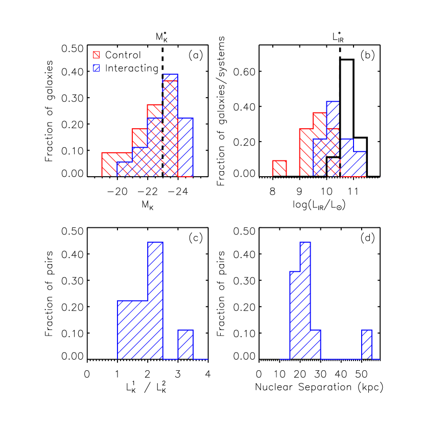
Figure 1.— Properties of the control and interacting galaxies samples: (a) $K$-band absolute magnitude; (b) $8-1000$µm infrared luminosity; (c) $K$-band luminosity ratio; and (d) nuclear separation. The control and interacting samples are shown as red and blue hatched histograms. In (b), the open histogram is the total system luminosity for the interacting sample. In (c), the convention is such that the luminosity ratio is always $>$1. The control and interacting samples are very similar in $M_{K}$, but the interacting galaxies have higher infrared luminosities. The interacting galaxies have luminosities near $L^{*}$, mass ratios in the range 1:1$-$1:2.5, and (projected) nuclear separations in the range $15-30$ kpc.

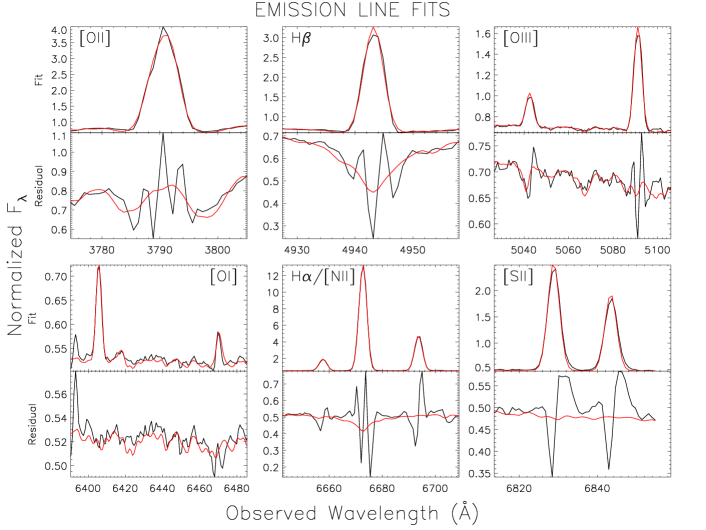
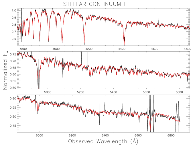
Figure 2.— Example fits to a high-flux and low-flux H II region spectrum from our sample (the latter has 1% of the H$\alpha$ flux of the former). These demonstrate the high fidelity of our fits over a large range of signal-to-noise. The top panels show close-ups of various emission line fits, with the residuals underneath each fit. The bottom panels show the fits to the stellar continuum, with the emission-line fits subtracted. Black is our data, and red is the fit. The spectra are shown in the observed frame.

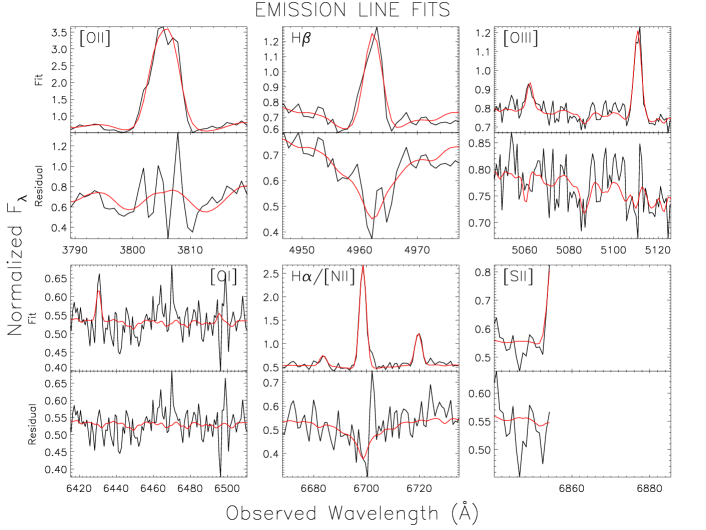
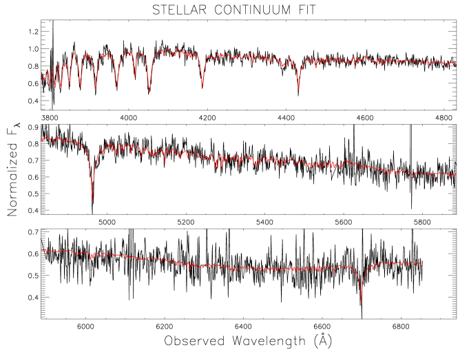
Figure 2.— Continued.

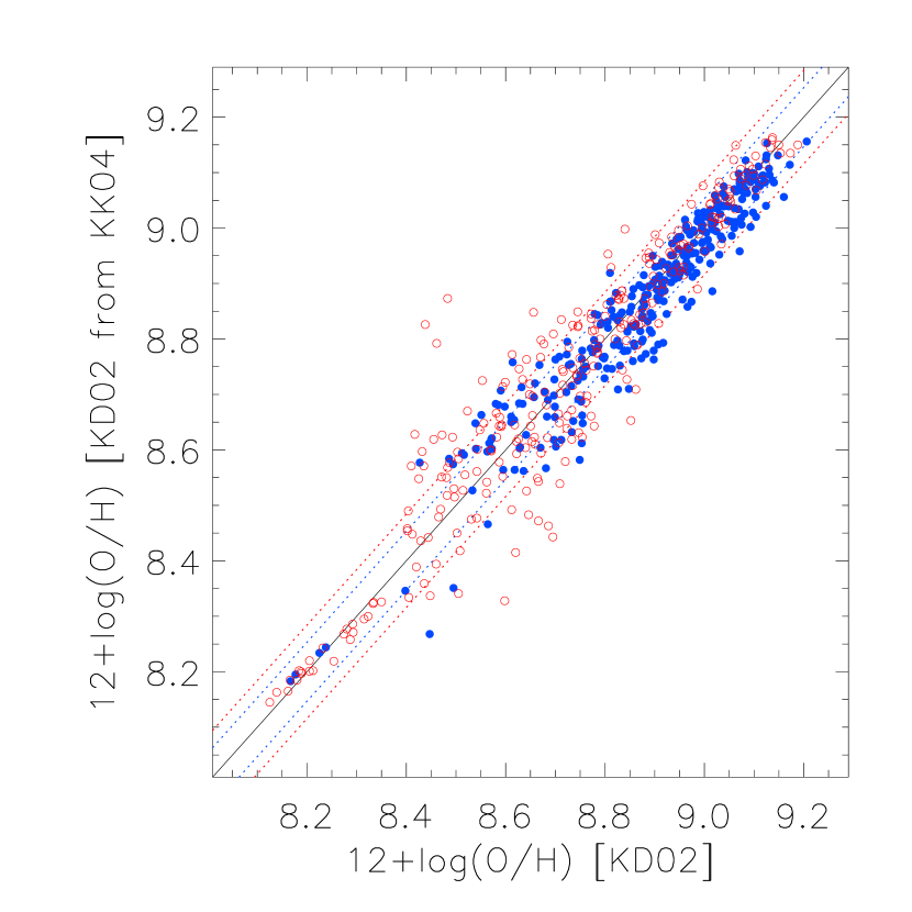
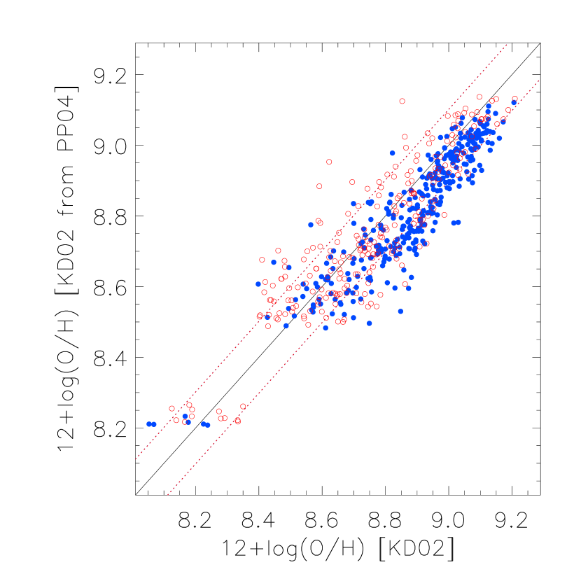
Figure 3.— Comparisons between different strong-line methods of calculating abundances, within the control sample (red open circles) and the interacting sample (blue filled circles). The diagonal black line shows equality, and the blue and red dashed lines show the RMS dispersion of each sample ($0.05-0.1$ dex) about equality. We compare our chosen diagnostic (KD02) with KK04 and PP04, converted into KD02 using Kewley & Ellison (2008) (§3.2). A small shift (0.05 dex) is seen toward higher metallicity when comparing KD02 and PP04, but this is well within the uncertainties of the calibrations and cross-calibrations. The good agreement between these methods points to the absence of strong systematic errors in our measurement of line fluxes.

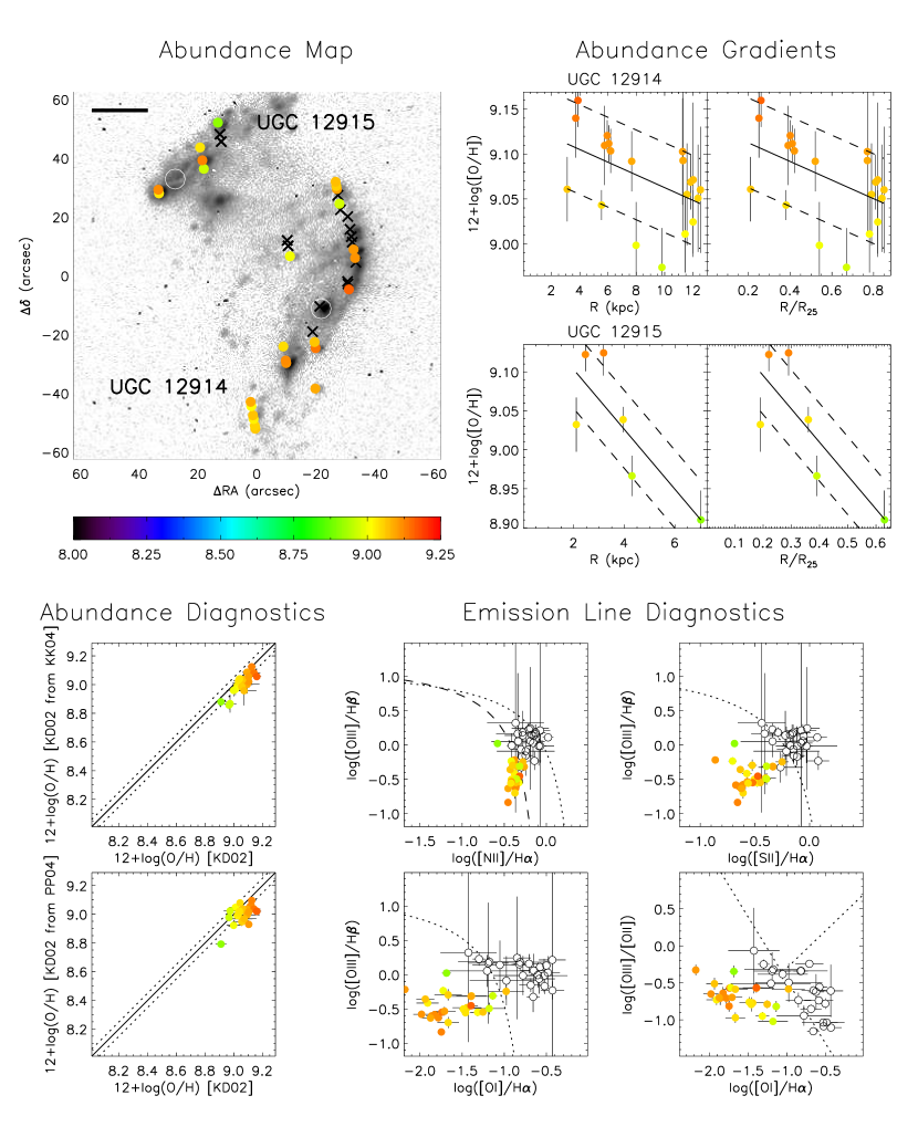
Figure 4.— Results of emission-line analysis of each system, including a map of the oxygen abundance from the [N II]/[O II] method, overplotted on an H$\alpha$ image (or F435W HST image in the cases of Arp 256 and Arp 298); abundance gradients for each galaxy, versus radius in kpc and radius normalized to R₂₅; comparisons between the KD02 abundance diagnostic and the KK04 and PP04 diagnostics; and the emission line ratio diagnostics from Kewley et al. (2006b). In each plot, the data points are colored according to the KD02 abundance (see color bar). The images show the near-infrared nuclear position as a white open circle, and a horizontal bar in the upper-left corner represents 5 kpc. The gradient panels show our formal fit and the average RMS (0.05 dex) around this. For the abundance comparisons, the KK04 and PP04 abundances are converted to the KD02 diagnostic using the conversions of Kewley & Ellison (2008). We overplot the line of equality and the RMS scatter in the Kewley & Ellison (2008) SDSS sample after this conversion ($\sim$0.05 dex). In the emission line diagnostics, points used in the abundance calculations are solid symbols; points rejected based on the [N II]/H$\alpha$ and [O I]/H$\alpha$ diagrams are open symbols. These rejected points are plotted as black crosses on the images.

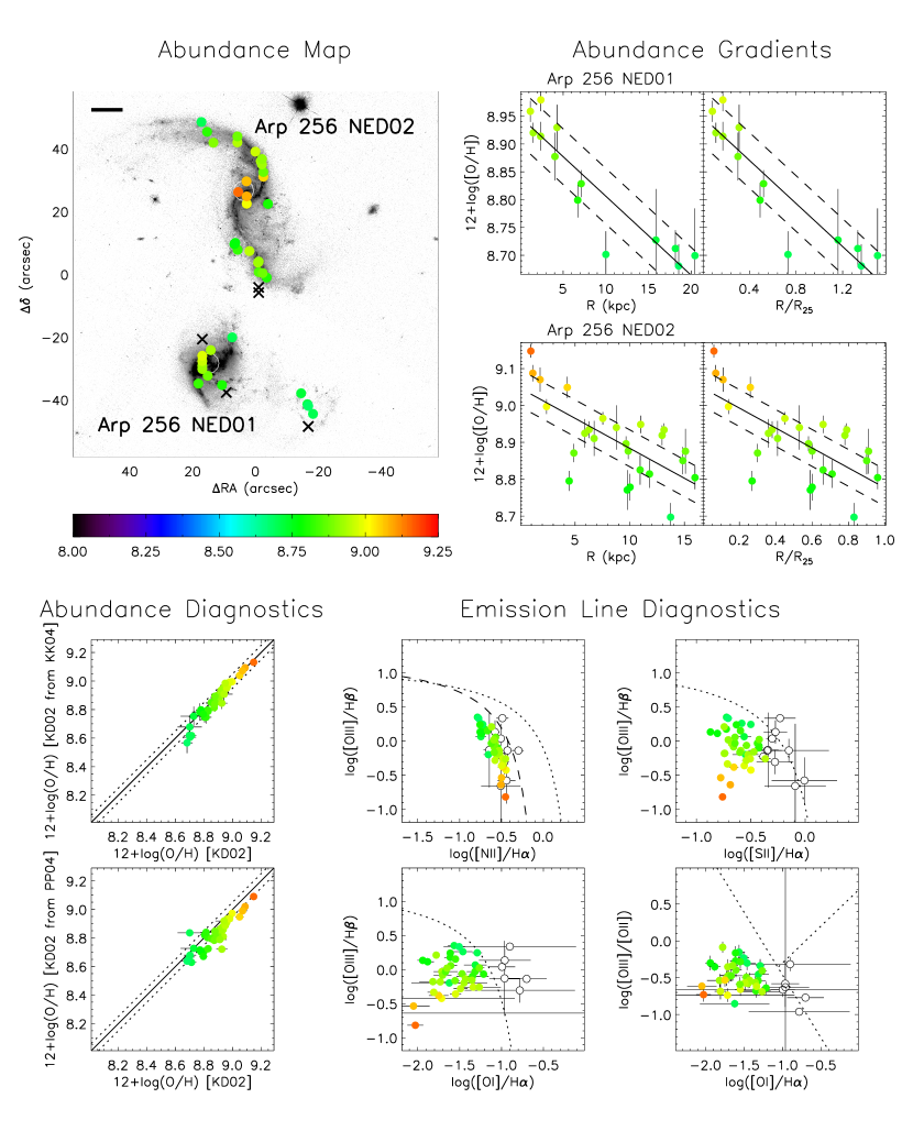
Figure 4.— Continued.

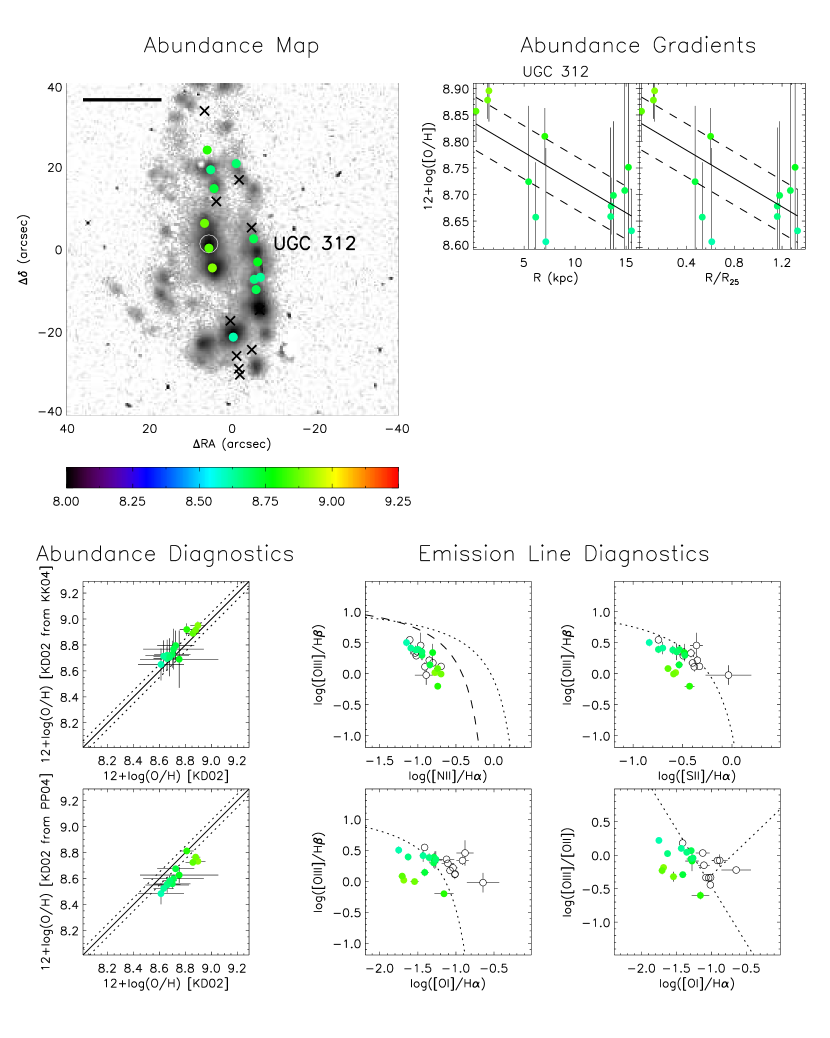
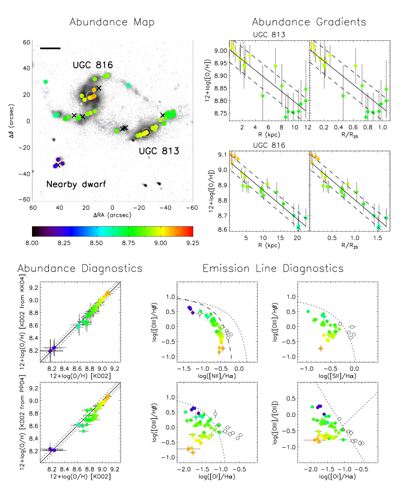
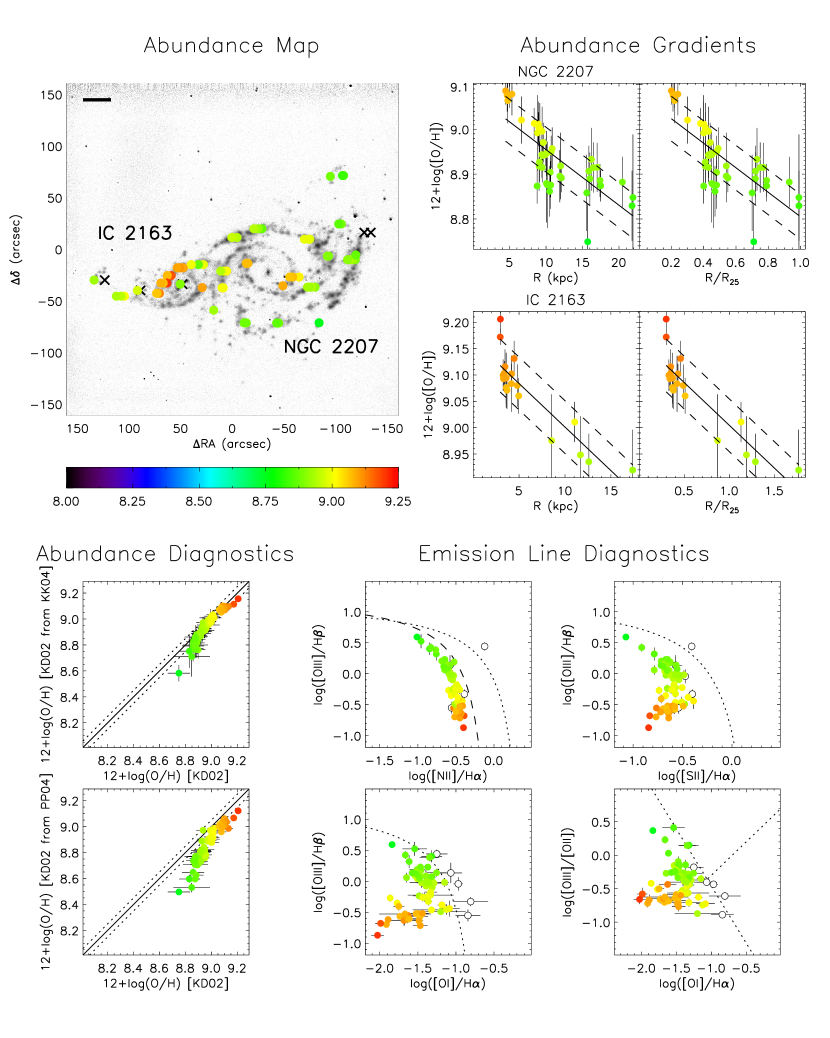
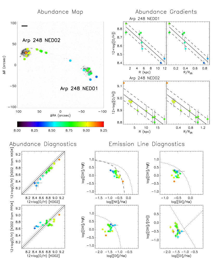
Figure 4.— Continued.

Figure 4.— Continued.

Figure 4.— Continued.

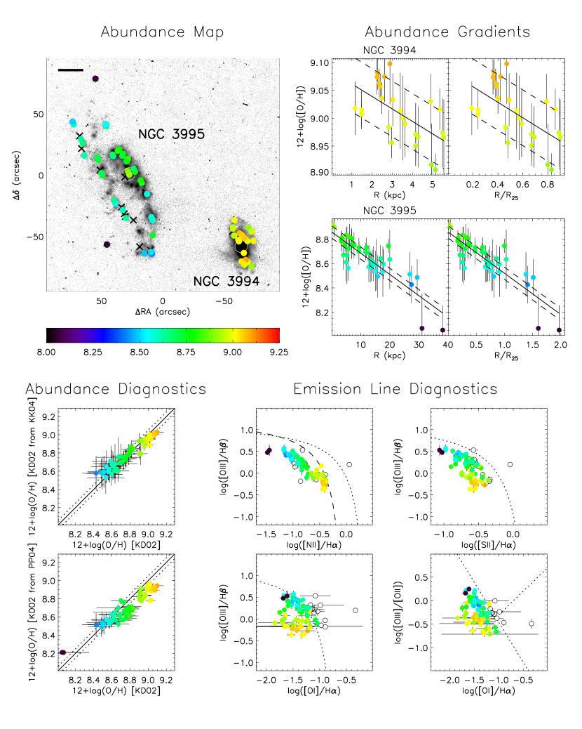
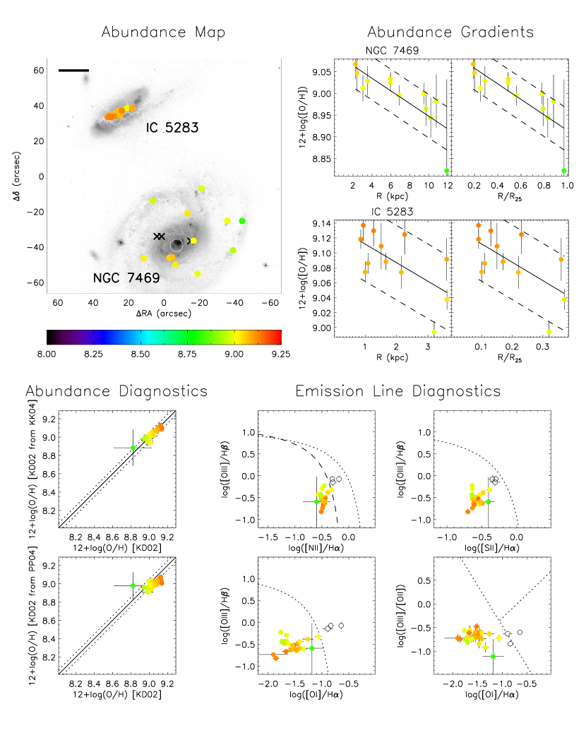
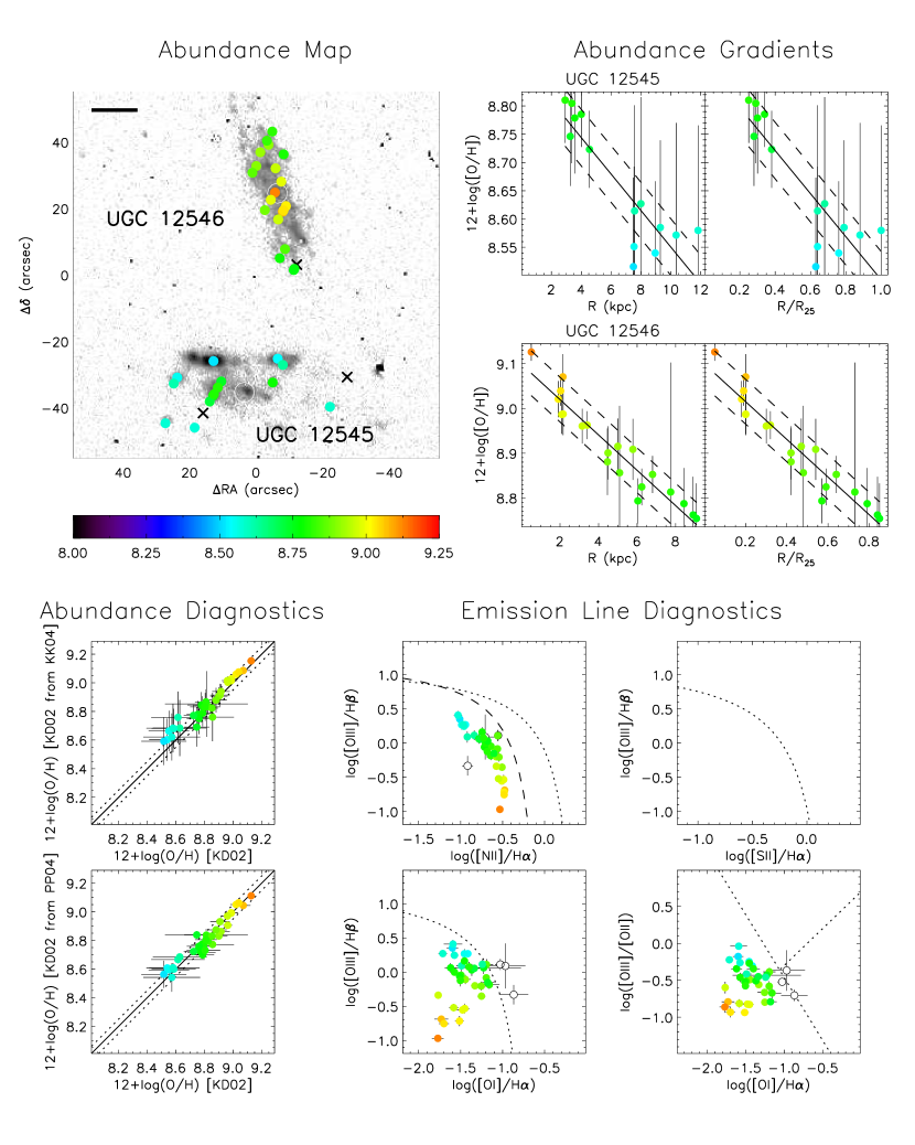
Figure 4.— Continued.

Figure 4.— Continued.

Figure 4.— Continued.

Figure 4.— Continued.

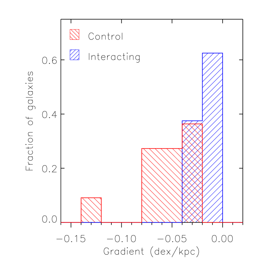
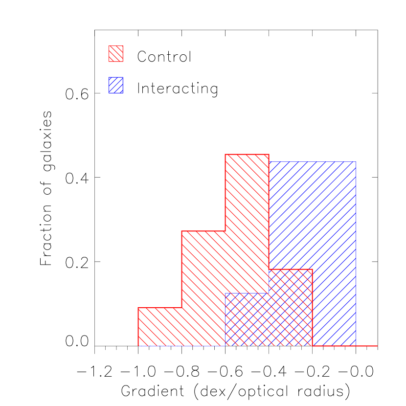
Figure 5.— Histograms of gradients in the control and interacting samples, in both dex/kpc (left) and dex/R₂₅ (right). The control sample has gradients that are twice as steep as the interacting sample.

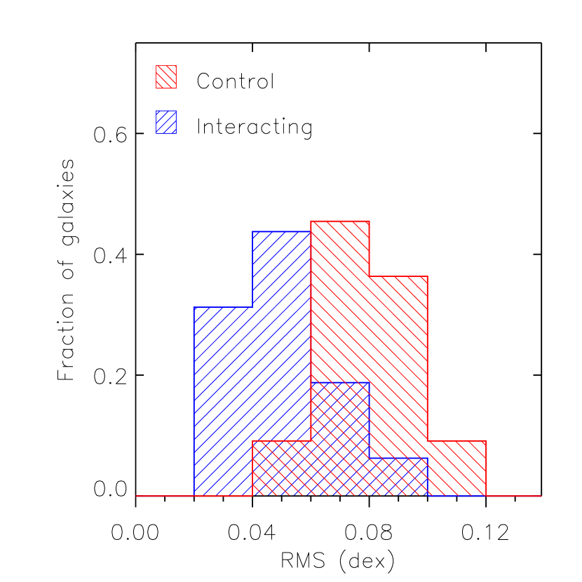
Figure 6.— Distribution of RMS residuals from a straight-line gradient, for the interacting and control samples. The interacting sample shows smaller, rather than larger, RMS residuals. This implies that the metallicity scatter in galaxies does not increase due to a merger; the observed decrease in the scatter is likely an artifact of the relative homogeneity of our data compared to the control sample.

Figure 7.— Gradients vs. galaxy properties: $K$-band and total infrared luminosities. Open circles are the control sample, and closed circles are the interacting sample. Arrows represent systems with unresolved infrared luminosity; in these cases the total system luminosity is an upper limit to the luminosity of each galaxy. No significant trends are apparent within either subsample.

Figure 8.— Gradients vs. system properties: nuclear separation, mass ratio (as traced by $K$-band luminosity), and total infrared luminosity. Pairs are connected by straight lines, and the most massive galaxy in each pair is circled. No significant trends are apparent.

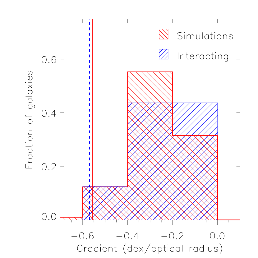
Figure 9.— Distribution of gradients in the interacting sample compared to the distribution predicted from the simulations of Rupke et al. (2010). The blue, dashed vertical line shows the average gradient in the control sample, and the red, solid vertical line shows the initial gradient for each simulation. The simulated distribution is computed assuming that the galaxies lie between first and second pericenter. Very good agreement is evident.

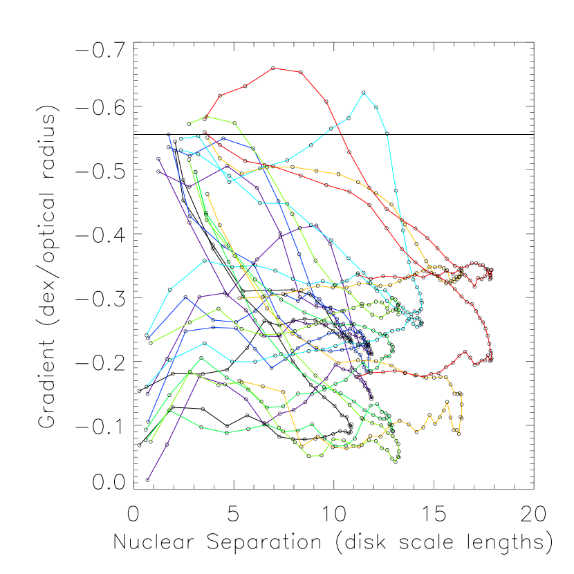
Figure 10.— Simulated dependence of gradient on (actual) nuclear separation between first and second pericenter (Rupke et al., 2010). Each point represents a time step for one of two galaxies in one of eight simulations. Points are connected for each galaxy, with a different color assigned to each simulation. The horizontal solid line is the initial gradient for each simulation. At the statistical level, no clear dependence of gradient on nuclear separation is expected, consistent with what is observed (Figure 8). It is also evident that in most systems, the gradient flattens quickly after first pericenter, as discussed in Rupke et al. (2010).

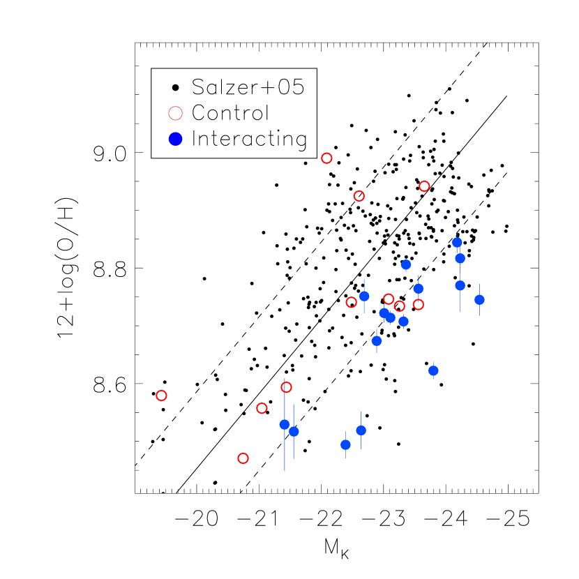
Figure 11.— Near-infrared luminosity-metallicity relation. The small black points are emission-line galaxies from Salzer et al. (2005); the open red circles are the control sample; and the filled blue circles are the interacting galaxies. Nuclear abundances for our sample are computed at $R=0.1$R₂₅. The solid line is the bisector of the Y on X and X on Y unweighted least-squares fits to the Salzer et al. (2005) sample, with RMS dispersion illustrated by the dashed lines. The control and interacting samples are shifted down by 0.3 dex so that the control sample lies atop the $L-Z$ relation. The interacting sample falls well beneath the $L-Z$ relation delineated by the control and Salzer et al. (2005) samples.

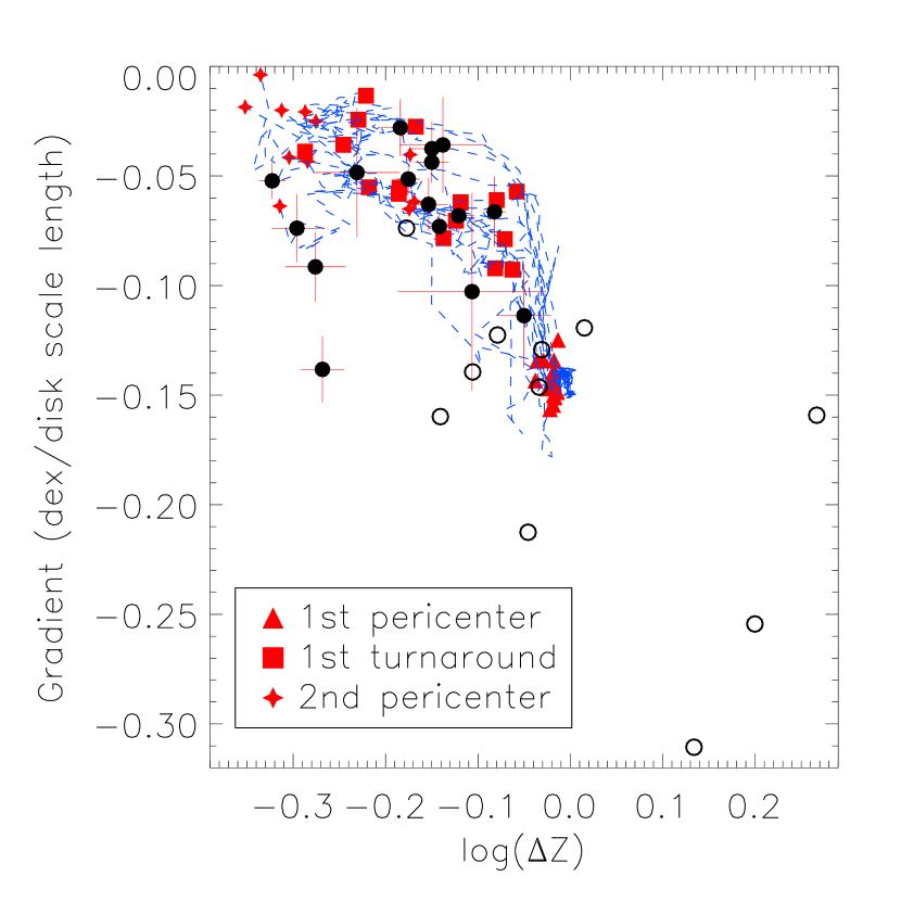
Figure 12.— Estimated offset from the $L-Z$ relation vs. metallicity gradient. Open circles are the control sample, and filled circles are the interacting sample. Dashed blue lines illustrate the time evolution in this phase space of the eight major merger models from Rupke et al. (2010). The models move from the center to the upper left. The triangles, squares, and star indicate various important points in the evolution of the simulated merger. The input gradient for the simulations is chosen to match the average gradient per stellar disk scale length from the control sample. Given both the measurement and systematic uncertainties in this procedure, there is excellent agreement between the data and models. The data are consistent with the typical system lying near first turnaround.

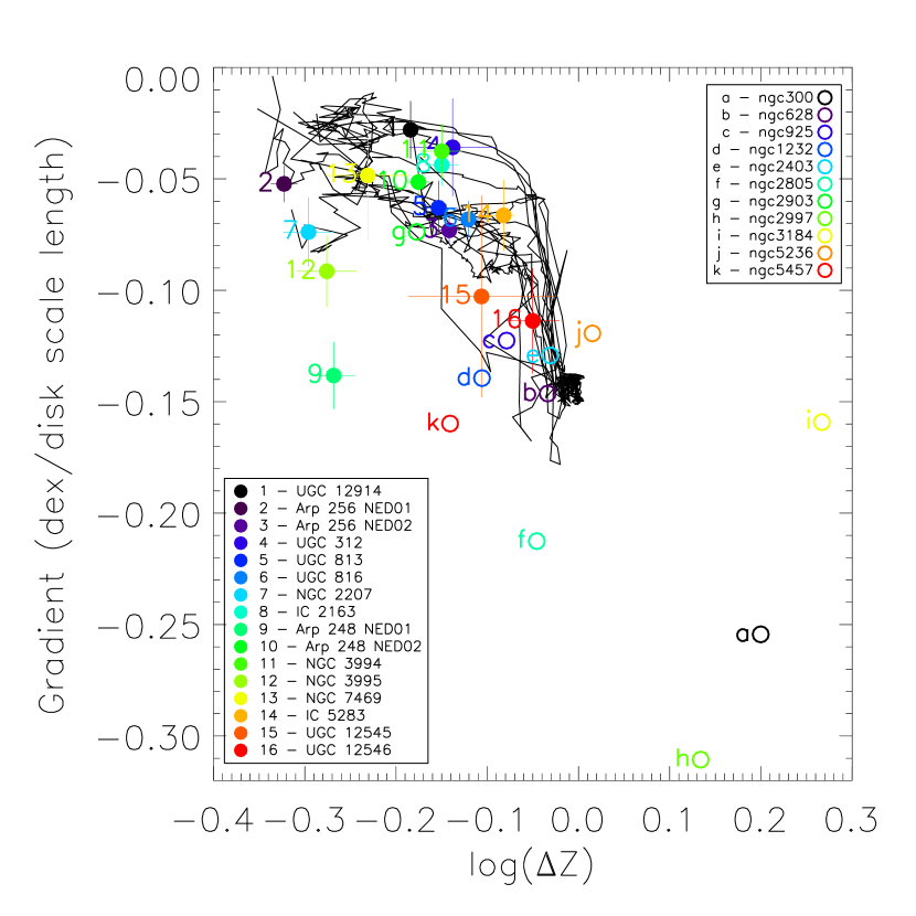
Figure 13.— Estimated offset from the $L-Z$ relation vs. metallicity gradient. See Figure 12 for more details. Individual galaxies are indicated.

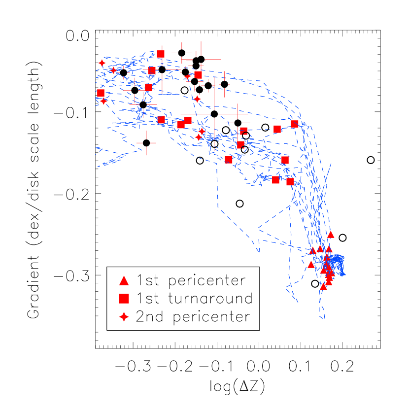
Figure 14.— Estimated offset from the $L-Z$ relation vs. metallicity gradient. See Figure 12 for more details. In the simulations displayed here, we used for initial conditions the steepest gradients observed in the control sample, and the corresponding $L-Z$ relation offsets. The overlap between data and simulations is poorer than in Fig. 12, and this scenario would require most of the pairs to lie near second pericenter rather than first turnaround. The data thus favor the shallower progenitor gradients illustrated in Fig. 12.

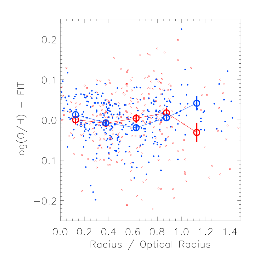
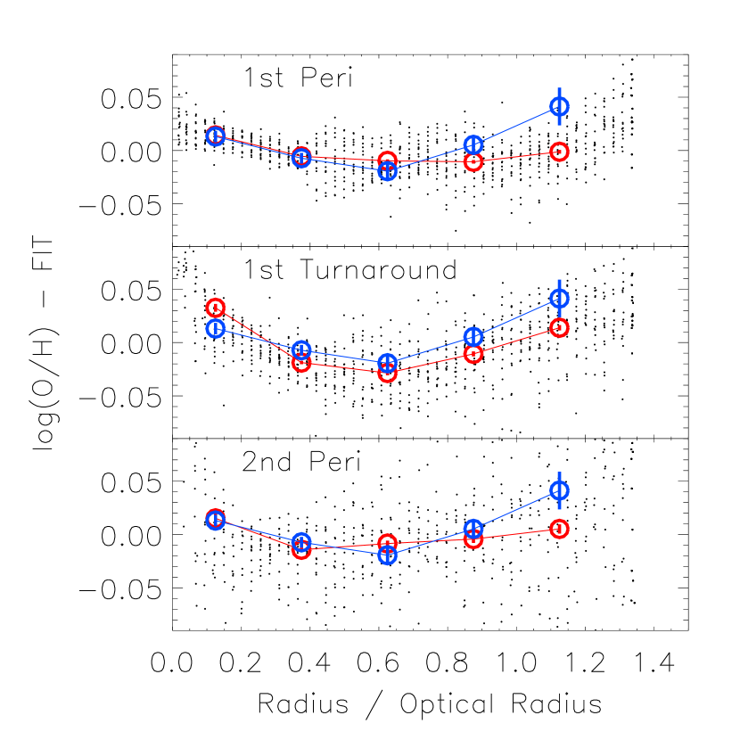
Figure 15.— (left) Metallicity residual from a straight line fit vs. radius for all H II regions in the control (open red circles) and the interacting (filled blue circles) samples. Binned points are averages over bins of size 0.25R₂₅, with the standard error shown as vertical error bars. The control sample is consistent with a mostly flat profile, while the interacting sample shows a “concave up” shape. (right) The same, but for the simulations (black points and red, open circles), with the binned data for the interacting sample overplotted. The best agreement in shape is found between the interacting sample and the simulations at first turnaround, which both have a “concave up” profile residual. Exact quantitative agreement is lacking, but this comparison is consistent with the idea that our sample lies on average near first turnaround.

Table 1Sample

Galaxy	System	$cz$	Nuc. Sep.	$M_{K}$	log($L_{\mathrm{IR}}$/$L_{\sun}$)	R25	$i$	PAnodes	Ref.
(1)	(2)	(3)	(4)	(5)	(6)	(7)	(8)	(9)	(10)
UGC 12914	VV254	4371	$\cdots$	-24.23	10.36	14.69	54	160	2,3,4
UGC 12915	VV254	4336	17.40	-23.70	10.76	11.11	73	135	2,3,4
Arp 256 NED02	Arp 256	8193	$\cdots$	-23.11	$\cdots$	16.58	0$-$45	70	1,3,4
Arp 256 NED01	Arp 256	8125	28.20	-23.80	11.35	13.66	61	80	1,3,4
UGC 312	HCG 2	4364	$\cdots$	-21.56	9.93	11.67	79	8	2
Mrk 552	HCG 2	4349	21.10	-22.33	10.38	$\cdots$	$\cdots$	$\cdots$	2
UGC 314	HCG 2	4271	65.40	-20.52	$\cdots$	$\cdots$	$\cdots$	$\cdots$	$\cdots$
UGC 813	WBL 036	5344	$\cdots$	-22.89	10.68	11.16	72	110	2
UGC 816	WBL 036	5188	16.50	-23.01	10.68	13.33	62	190	2
CGCG 551-011	WBL 036	5373	42.60	-23.27	$\cdots$	$\cdots$	$\cdots$	$\cdots$	2
NGC 2207	NGC 2207/IC 2163	2741	$\cdots$	-24.54	11.00	22.11	35	140	3,4
IC 2163	NGC 2207/IC 2163	2765	15.80	-24.18	$\cdots$	9.80	35	128	3,4
Arp 248 NED01	Arp 248	5167	$\cdots$	-22.39	10.66	13.90	66	43	1
Arp 248 NED02	Arp 248	5167	54.60	-23.32	10.66	13.27	0$-$45	109	1
Arp 248 NED03	Arp 248	5276	93.10	-20.82	$\cdots$	$\cdots$	$\cdots$	$\cdots$	1
NGC 3994	Arp 313	3086	$\cdots$	-23.56	10.55	6.18	58	10	1,2,3,4
NGC 3995	Arp 313	3254	24.70	-22.64	10.42	19.40	69	45	1,2,3,4
NGC 3991	Arp 313	3192	50.10	-22.51	10.26	$\cdots$	$\cdots$	$\cdots$	4
NGC 7469	Arp 298	4892	$\cdots$	-24.23	11.46	12.22	30	127	1,3,4
IC 5283	Arp 298	4804	23.30	-23.36	$\cdots$	9.90	60	105	1,3,4
UGC 12545	WBL 713	5754	$\cdots$	-21.41	10.28	11.81	63	85	2
UGC 12546	WBL 713	6055	21.90	-22.69	10.28	10.64	63	20	2

References. — 1 = Arp (1966); 2 = Barton et al. (2000); 3 = Sanders et al. (2003); 4 = Surace et al. (2004)

Note. — Col.(1): Galaxy name. Col.(2): System label from optical identification. In order of preference: Arp = Arp (1966); VV = Vorontsov-Velyaminov (1977); HCG = Hickson Compact Group = Hickson (1982); WBL = White et al. (1999) catalog of poor clusters. Col.(3): Redshift from NED, in km s^-1. Col.(4): Projected nuclear separation from first galaxy listed for system, in kpc, using. Col.(5): $K$-band magnitude down to 20 mag/arcsec² isophote, from 2MASS. Col.(6): 8$-$1000µm luminosity, determined using the formula in Sanders & Mirabel (1996) and fluxes from Surace et al. (2004), the IRAS Faint Source Catalog, or Johnson et al. (2007) in the case of HCG 2. Col.(7): $B$-band optical radius from 25 mag/arcsec² isophote, in kpc, from HyperLeda (Paturel et al., 2003). Col.(8): Inclination in degrees, from HyperLeda except for Arp 248 NED02 and Arp 256 NED02. For these cases, we assume 30^∘; the actual inclination is in the range $0-45^{\circ}$. Col.(9): Position angle of the galaxy line of nodes, in degrees east of north; from HyperLeda except for Arp 256 and WBL 036 (used H I data from Chen et al. 2002 and Condon et al. 2002). Col.(10): Sample selection reference (§2.1).

Table 2Control Sample

Galaxy	Type	Distance	Dist. Ref.	$M_{K}$	log($L_{\mathrm{IR}}$/$L_{\sun}$)	R25	Rd	Rd Ref.	$i$	PAnodes	$i$/PA Ref.	H II Ref.
(1)	(2)	(3)	(4)	(5)	(6)	(7)	(8)	(9)	(10)	(11)	(12)	(13)
NGC  300	SAd	2.08	a	-19.43	8.43	5.90	2.26	B	40	114	aa	1
NGC  628 (M74)	SAc	8.59	b	-22.48	9.82	13.08	3.57	A	7	25	cc	6,7
NGC  925	SABd	7.38	e	-20.75	9.21	12.04	2.60	D	61	107	aa	7
NGC 1232	SABc	14.50	d	-23.08	9.91	14.59	4.51	C	33	270	aa,ee	3,7
NGC 2403	SABcd	3.16	a	-21.05	9.19	9.17	1.72	C	60	127	aa	4,7
NGC 2805	SABd	28.00	c	-21.44	9.68	14.42	8.96	E	36	290	aa,bb	7
NGC 2903	SABbc	8.55	e	-23.56	10.22	14.95	3.09	E	56	23	aa	3,7
NGC 2997	SABc	7.08	e	-22.61	9.82	11.55	4.84	F	41	110	aa	3
NGC 3184	SABcd	8.70	c	-22.09	9.48	9.60	2.59	G	24	135	aa	7
NGC 5236 (M83)	SABc	4.92	a	-23.66	10.37	10.34	2.89	F	27	45	aa	2,3
NGC 5457 (M101)	SABcd	6.96	a	-23.26	10.23	29.19	5.19	E	37	18	dd	5

References. — Distances: a = Jacobs et al. (2009); b = Herrmann et al. (2008); c = Tully (1988); d = Tully et al. (2009); e = Tully et al. (2008). R₂₅: A = Boroson (1981); B = Carignan (1985); C = Elmegreen & Elmegreen (1984); D = Elmegreen & Elmegreen (1985); E = Koopmann et al. (2006); F = Simien & de Vaucouleurs (1986); G = van Zee et al. (1998). $i$/PA: aa = HyperLeda (Paturel et al. 2003); bb = Bosma et al. (1980); cc = Kamphuis & Briggs (1992); dd = Kennicutt & Garnett (1996); ee = van Zee & Bryant (1999). H II regions: 1 = Bresolin et al. (2009a); 2 = Bresolin et al. (2009b); 3 = Bresolin et al. (2005); 4 = Garnett et al. (1997); 5 = Kennicutt et al. (2003); 6 = McCall et al. (1985); 7 = van Zee et al. (1998).

Note. — Col.(1): Galaxy name. Col.(2): Morphological type, from NED. Col.(3-4): Distance, in Mpc, and reference. Col.(5): $K$-band magnitude down to 20 mag/arcsec² isophote, from 2MASS. Col.(6): 8$-$1000µm luminosity, determined using the formula in Sanders & Mirabel (1996) and infrared fluxes from NED. Col.(7): $B$-band optical radius from 25 mag/arcsec² isophote, in kpc, from HyperLeda (Paturel et al. 2003; except for M101, which is from the RC3). Col.(8-9): $B$-band stellar exponential disk scale length, in kpc, and reference. Col. (10-12): Inclination, in degrees; position angle of the galaxy line of nodes, in degrees east of north; and reference for these. Col.(13): Reference for emission-line data.

Table 3Gradient Fits

Galaxy	$N_{reg}$	$\Delta$(dex/kpc)	$\Delta$(dex/R25)	Intercept
(1)	(2)	(3)	(4)	(5)
Control Sample
NGC 300	27	-0.1246	-0.664	8.95
NGC 628	25	-0.0410	-0.536	9.10
NGC 925	44	-0.0471	-0.568	8.83
NGC 1232	22	-0.0310	-0.451	9.10
NGC 2403	25	-0.0750	-0.689	8.93
NGC 2805	15	-0.0237	-0.342	8.93
NGC 2903	17	-0.0239	-0.357	9.08
NGC 2997	14	-0.0642	-0.741	9.30
NGC 3184	17	-0.0613	-0.590	9.35
NGC 5236	38	-0.0413	-0.427	9.29
NGC 5457	25	-0.0310	-0.899	9.13
Interacting Galaxies Sample
UGC 12914	20	-0.0071$\pm$ 0.0033	-0.104$\pm$ 0.048	9.13$\pm$ 0.02
Arp 256 NED01	13	-0.0142$\pm$ 0.0022	-0.193$\pm$ 0.031	8.95$\pm$ 0.01
Arp 256 NED02	25	-0.0162$\pm$ 0.0014	-0.271$\pm$ 0.023	9.05$\pm$ 0.01
UGC 312	13	-0.0114$\pm$ 0.0070	-0.133$\pm$ 0.081	8.84$\pm$ 0.05
UGC 813	20	-0.0210$\pm$ 0.0040	-0.233$\pm$ 0.045	9.00$\pm$ 0.02
UGC 816	21	-0.0189$\pm$ 0.0023	-0.252$\pm$ 0.030	9.05$\pm$ 0.02
NGC 2207	43	-0.0124$\pm$ 0.0026	-0.273$\pm$ 0.057	9.08$\pm$ 0.03
IC 2163	19	-0.0165$\pm$ 0.0036	-0.162$\pm$ 0.035	9.17$\pm$ 0.02
Arp 248 NED01	8	-0.0368$\pm$ 0.0040	-0.512$\pm$ 0.056	8.85$\pm$ 0.02
Arp 248 NED02	11	-0.0144$\pm$ 0.0020	-0.190$\pm$ 0.026	9.03$\pm$ 0.01
NGC 3994	25	-0.0224$\pm$ 0.0072	-0.139$\pm$ 0.045	9.08$\pm$ 0.02
NGC 3995	41	-0.0175$\pm$ 0.0030	-0.339$\pm$ 0.059	8.86$\pm$ 0.03
NGC 7469	12	-0.0146$\pm$ 0.0089	-0.179$\pm$ 0.109	9.09$\pm$ 0.05
IC 5283	12	-0.0249$\pm$ 0.0060	-0.246$\pm$ 0.059	9.14$\pm$ 0.01
UGC 12545	14	-0.0323$\pm$ 0.0142	-0.381$\pm$ 0.168	8.87$\pm$ 0.08
UGC 12546	20	-0.0395$\pm$ 0.0082	-0.421$\pm$ 0.087	9.10$\pm$ 0.03

Note. — Col.(1): Galaxy name. Col.(2): Number of H II regions used in fit. Col.(3-4): Radial oxygen abundance gradient, in dex/kpc and dex/R₂₅. Col.(5). Intercept of oxygen abundance vs. radius fit, expressed as 12$+$log(O/H).

References

- Allen et al. (2008) Allen, M. G., Groves, B. A., Dopita, M. A., Sutherland, R. S., & Kewley, L. J. 2008, ApJS, 178, 20, arXiv:0805.0204
- Arp (1966) Arp, H. 1966, Atlas of peculiar galaxies (Pasadena: California Inst. Technology), ADS
- Barnes (1998) Barnes, J. E. 1998, in Saas-Fee Advanced Course 26: Galaxies: Interactions and Induced Star Formation, ed. R. C. Kennicutt Jr., F. Schweizer, J. E. Barnes, D. Friedli, L. Martinet, & D. Pfenniger, 275, ADS
- Barnes (2004) Barnes, J. E. 2004, MNRAS, 350, 798, arXiv:astro-ph/0402248
- Barnes & Hernquist (1996) Barnes, J. E., & Hernquist, L. 1996, ApJ, 471, 115, ADS
- Barton et al. (2000) Barton, E. J., Geller, M. J., & Kenyon, S. J. 2000, ApJ, 530, 660, arXiv:astro-ph/9909217
- Boroson (1981) Boroson, T. 1981, ApJS, 46, 177, ADS
- Bosma et al. (1980) Bosma, A., Casini, C., Heidmann, J., van der Hulst, J. M., & van Woerden, H. 1980, A&A, 89, 345, ADS
- Bresolin et al. (2009a) Bresolin, F., Gieren, W., Kudritzki, R., Pietrzyński, G., Urbaneja, M. A., & Carraro, G. 2009a, ApJ, 700, 309, arXiv:0905.2791
- Bresolin et al. (2009b) Bresolin, F., Ryan-Weber, E., Kennicutt, R. C., & Goddard, Q. 2009b, ApJ, 695, 580, arXiv:0901.1127
- Bresolin et al. (2005) Bresolin, F., Schaerer, D., González Delgado, R. M., & Stasińska, G. 2005, A&A, 441, 981, ADS
- Brooks et al. (2007) Brooks, A. M., Governato, F., Booth, C. M., Willman, B., Gardner, J. P., Wadsley, J., Stinson, G., & Quinn, T. 2007, ApJ, 655, L17, arXiv:astro-ph/0609620
- Bundy et al. (2009) Bundy, K., Fukugita, M., Ellis, R. S., Targett, T. A., Belli, S., & Kodama, T. 2009, ApJ, 697, 1369, arXiv:0902.1188
- Cardelli et al. (1989) Cardelli, J. A., Clayton, G. C., & Mathis, J. S. 1989, ApJ, 345, 245, ADS
- Carignan (1985) Carignan, C. 1985, ApJS, 58, 107, ADS
- Charlot & Longhetti (2001) Charlot, S., & Longhetti, M. 2001, MNRAS, 323, 887, arXiv:astro-ph/0101097
- Chen et al. (2002) Chen, J., Lo, K. Y., Gruendl, R. A., Peng, M., & Gao, Y. 2002, AJ, 123, 720, arXiv:astro-ph/0110627
- Chien et al. (2007) Chien, L.-H., Barnes, J. E., Kewley, L. J., & Chambers, K. C. 2007, ApJ, 660, L105, arXiv:astro-ph/0703510
- Condon et al. (2002) Condon, J. J., Helou, G., & Jarrett, T. H. 2002, AJ, 123, 1881, ADS
- Condon et al. (1993) Condon, J. J., Helou, G., Sanders, D. B., & Soifer, B. T. 1993, AJ, 105, 1730, ADS
- Dalcanton (2007) Dalcanton, J. J. 2007, ApJ, 658, 941, arXiv:astro-ph/0608590
- de Ravel et al. (2009) de Ravel, L. et al. 2009, A&A, 498, 379, arXiv:0807.2578
- Di Matteo et al. (2009) Di Matteo, P., Pipino, A., Lehnert, M. D., Combes, F., & Semelin, B. 2009, A&A, 499, 427, arXiv:0903.2846
- Dutil & Roy (1999) Dutil, Y., & Roy, J. 1999, ApJ, 516, 62, ADS
- Ekta & Chengalur (2010) Ekta, B., & Chengalur, J. N. 2010, MNRAS, 406, 1238, arXiv:1003.6026
- Ellison et al. (2008) Ellison, S. L., Patton, D. R., Simard, L., & McConnachie, A. W. 2008, AJ, 135, 1877, arXiv:0803.0161
- Elmegreen & Elmegreen (1985) Elmegreen, B. G., & Elmegreen, D. M. 1985, ApJ, 288, 438, ADS
- Elmegreen et al. (2000) Elmegreen, B. G. et al. 2000, AJ, 120, 630, arXiv:astro-ph/0007200
- Elmegreen et al. (1995) Elmegreen, B. G., Sundin, M., Kaufman, M., Brinks, E., & Elmegreen, D. M. 1995, ApJ, 453, 139, ADS
- Elmegreen & Elmegreen (1984) Elmegreen, D. M., & Elmegreen, B. G. 1984, ApJS, 54, 127, ADS
- Friedli et al. (1994) Friedli, D., Benz, W., & Kennicutt, R. 1994, ApJ, 430, L105, ADS
- Garnett et al. (1997) Garnett, D. R., Shields, G. A., Skillman, E. D., Sagan, S. P., & Dufour, R. J. 1997, ApJ, 489, 63, ADS
- González Delgado et al. (2005) González Delgado, R. M., Cerviño, M., Martins, L. P., Leitherer, C., & Hauschildt, P. H. 2005, MNRAS, 357, 945, arXiv:astro-ph/0501204
- Herrmann et al. (2008) Herrmann, K. A., Ciardullo, R., Feldmeier, J. J., & Vinciguerra, M. 2008, ApJ, 683, 630, arXiv:0805.1074
- Hickson (1982) Hickson, P. 1982, ApJ, 255, 382, ADS
- Jacobs et al. (2009) Jacobs, B. A., Rizzi, L., Tully, R. B., Shaya, E. J., Makarov, D. I., & Makarova, L. 2009, AJ, 138, 332, arXiv:0902.3675
- Johnson et al. (2007) Johnson, K. E., Hibbard, J. E., Gallagher, S. C., Charlton, J. C., Hornschemeier, A. E., Jarrett, T. H., & Reines, A. E. 2007, AJ, 134, 1522, arXiv:0706.4461
- Kamphuis & Briggs (1992) Kamphuis, J., & Briggs, F. 1992, A&A, 253, 335, ADS
- Kauffmann et al. (2003) Kauffmann, G. et al. 2003, MNRAS, 346, 1055, arXiv:astro-ph/0304239
- Kennicutt et al. (2003) Kennicutt, Jr., R. C., Bresolin, F., & Garnett, D. R. 2003, ApJ, 591, 801, arXiv:astro-ph/0303452
- Kennicutt & Garnett (1996) Kennicutt, Jr., R. C., & Garnett, D. R. 1996, ApJ, 456, 504, ADS
- Kewley & Dopita (2002) Kewley, L. J., & Dopita, M. A. 2002, ApJS, 142, 35, arXiv:astro-ph/0206495
- Kewley et al. (2001) Kewley, L. J., Dopita, M. A., Sutherland, R. S., Heisler, C. A., & Trevena, J. 2001, ApJ, 556, 121, arXiv:astro-ph/0106324
- Kewley & Ellison (2008) Kewley, L. J., & Ellison, S. L. 2008, ApJ, 681, 1183, arXiv:0801.1849
- Kewley et al. (2006a) Kewley, L. J., Geller, M. J., & Barton, E. J. 2006a, AJ, 131, 2004, arXiv:astro-ph/0511119
- Kewley et al. (2006b) Kewley, L. J., Groves, B., Kauffmann, G., & Heckman, T. 2006b, MNRAS, 372, 961, arXiv:astro-ph/0605681
- Kewley et al. (2010) Kewley, L. J., Rupke, D. S. N., Zahid, J., Geller, M. J., Barton, B. J., & Chien, L.-H. 2010, ApJ, in press, arXiv:1008.2204
- Kobulnicky & Kewley (2004) Kobulnicky, H. A., & Kewley, L. J. 2004, ApJ, 617, 240, arXiv:astro-ph/0408128
- Kochanek et al. (2001) Kochanek, C. S. et al. 2001, ApJ, 560, 566, arXiv:astro-ph/0011456
- Koopmann et al. (2006) Koopmann, R. A., Haynes, M. P., & Catinella, B. 2006, AJ, 131, 716, arXiv:astro-ph/0510374
- Köppen et al. (2007) Köppen, J., Weidner, C., & Kroupa, P. 2007, MNRAS, 375, 673, arXiv:astro-ph/0611723
- Lee et al. (2004) Lee, J. C., Salzer, J. J., & Melbourne, J. 2004, ApJ, 616, 752, arXiv:astro-ph/0408342
- Maraston (2005) Maraston, C. 2005, MNRAS, 362, 799, arXiv:astro-ph/0410207
- Martin (1995) Martin, P. 1995, AJ, 109, 2428, ADS
- Martin & Roy (1995) Martin, P., & Roy, J. 1995, ApJ, 445, 161, ADS
- McCall et al. (1985) McCall, M. L., Rybski, P. M., & Shields, G. A. 1985, ApJS, 57, 1, ADS
- McCarthy et al. (1998) McCarthy, J. K. et al. 1998, in SPIE Conference, Vol. 3355, SPIE Conference Series, ed. S. D’Odorico, 81–92, ADS
- Michel-Dansac et al. (2008) Michel-Dansac, L., Lambas, D. G., Alonso, M. S., & Tissera, P. 2008, MNRAS, 386, L82, arXiv:0802.3904
- Mihos & Hernquist (1996) Mihos, J. C., & Hernquist, L. 1996, ApJ, 464, 641, arXiv:astro-ph/9512099
- Montuori et al. (2010) Montuori, M., Di Matteo, P., Lehnert, M. D., Combes, F., & Semelin, B. 2010, ArXiv e-prints, arXiv:1003.1374
- Moustakas & Kennicutt (2006) Moustakas, J., & Kennicutt, Jr., R. C. 2006, ApJS, 164, 81, arXiv:astro-ph/0511729
- Oke et al. (1995) Oke, J. B. et al. 1995, PASP, 107, 375, ADS
- Paturel et al. (2003) Paturel, G., Petit, C., Prugniel, P., Theureau, G., Rousseau, J., Brouty, M., Dubois, P., & Cambrésy, L. 2003, A&A, 412, 45, ADS
- Peeples et al. (2009) Peeples, M. S., Pogge, R. W., & Stanek, K. Z. 2009, ApJ, 695, 259, arXiv:0809.0896
- Pettini & Pagel (2004) Pettini, M., & Pagel, B. E. J. 2004, MNRAS, 348, L59, arXiv:astro-ph/0401128
- Rich et al. (2010) Rich, J. A., Dopita, M. A., Kewley, L. J., & Rupke, D. S. N. 2010, ApJ, in press, arXiv:1007.3495
- Robaina et al. (2010) Robaina, A. R., Bell, E. F., van der Wel, A., Somerville, R. S., Skelton, R. E., McIntosh, D. H., Meisenheimer, K., & Wolf, C. 2010, ArXiv e-prints, arXiv:1002.4193
- Roy & Walsh (1997) Roy, J., & Walsh, J. R. 1997, MNRAS, 288, 715, arXiv:astro-ph/9705032
- Rupke et al. (2010) Rupke, D. S. N., Kewley, L. J., & Barnes, J. E. 2010, ApJ, 710, L156, arXiv:1001.1728
- Rupke et al. (2008) Rupke, D. S. N., Veilleux, S., & Baker, A. J. 2008, ApJ, 674, 172, arXiv:0708.1766
- Salzer et al. (2005) Salzer, J. J., Lee, J. C., Melbourne, J., Hinz, J. L., Alonso-Herrero, A., & Jangren, A. 2005, ApJ, 624, 661, arXiv:astro-ph/0502202
- Sanders et al. (2003) Sanders, D. B., Mazzarella, J. M., Kim, D.-C., Surace, J. A., & Soifer, B. T. 2003, AJ, 126, 1607, arXiv:astro-ph/0306263
- Sanders & Mirabel (1996) Sanders, D. B., & Mirabel, I. F. 1996, ARA&A, 34, 749, ADS
- Sanders et al. (1991) Sanders, D. B., Scoville, N. Z., & Soifer, B. T. 1991, ApJ, 370, 158, ADS
- Simien & de Vaucouleurs (1986) Simien, F., & de Vaucouleurs, G. 1986, ApJ, 302, 564, ADS
- Sol Alonso et al. (2010) Sol Alonso, M., Michel-Dansac, L., & Lambas, D. G. 2010, A&A, 514, A57+, arXiv:1001.4605
- Surace et al. (2004) Surace, J. A., Sanders, D. B., & Mazzarella, J. M. 2004, AJ, 127, 3235, arXiv:astro-ph/0402531
- Tremonti et al. (2004) Tremonti, C. A. et al. 2004, ApJ, 613, 898, arXiv:astro-ph/0405537
- Tully (1988) Tully, R. B. 1988, Nearby Galaxies Catalog (Cambridge and New York, Cambridge University Press, 1988), ADS
- Tully et al. (2009) Tully, R. B., Rizzi, L., Shaya, E. J., Courtois, H. M., Makarov, D. I., & Jacobs, B. A. 2009, AJ, 138, 323, ADS
- Tully et al. (2008) Tully, R. B., Shaya, E. J., Karachentsev, I. D., Courtois, H. M., Kocevski, D. D., Rizzi, L., & Peel, A. 2008, ApJ, 676, 184, arXiv:0705.4139
- van Zee & Bryant (1999) van Zee, L., & Bryant, J. 1999, AJ, 118, 2172, arXiv:astro-ph/9907278
- van Zee et al. (1998) van Zee, L., Salzer, J. J., Haynes, M. P., O’Donoghue, A. A., & Balonek, T. J. 1998, AJ, 116, 2805, arXiv:astro-ph/9808315
- Vila-Costas & Edmunds (1992) Vila-Costas, M. B., & Edmunds, M. G. 1992, MNRAS, 259, 121, ADS
- Vorontsov-Velyaminov (1977) Vorontsov-Velyaminov, B. A. 1977, A&AS, 28, 1, ADS
- White et al. (1999) White, R. A., Bliton, M., Bhavsar, S. P., Bornmann, P., Burns, J. O., Ledlow, M. J., & Loken, C. 1999, AJ, 118, 2014, arXiv:astro-ph/9907283
- Zahid et al. (2010) Zahid, H. J., Kewley, L. J., & Bresolin, F. 2010, ApJ, submitted, arXiv:1006.4877
- Zaritsky et al. (1994) Zaritsky, D., Kennicutt, Jr., R. C., & Huchra, J. P. 1994, ApJ, 420, 87, ADS