Will the tachyonic Universe survive the Big Brake?

Abstract

We investigate a Friedmann universe filled with a tachyon scalar field, which behaves as dustlike matter in the past, while it is able to accelerate the expansion rate of the universe at late times. The comparison with type Ia supernovae (SNIa) data allows for evolutions driving the universe into a Big Brake. Some of the evolutions leading to a Big Brake exhibit a large variation of the equation of state parameter at low redshifts which is potentially observable with future data though hardly detectable with present SNIa data. The soft Big Brake singularity occurs at finite values of the scale factor, vanishing energy density and Hubble parameter, but diverging deceleration and infinite pressure. We show that the geodesics can be continued through the Big Brake and that our model universe will recollapse eventually in a Big Crunch. Although the time to the Big Brake strongly depends on the present values of the tachyonic field and of its time derivative, the time from the Big Brake to the Big Crunch represents a kind of invariant timescale for all field parameters allowed by SNIa.

I Introduction

Dark energy (DE) models aim to explain the accelerated expansion rate of the universe at late times. This phenomenon was originally discovered using supernovae Ia (SNIa) data cosm and has since then been confirmed by many other observations (see e.g. Tsuji and references therein). Still, the nature of dark energy, and the precise physical mechanism producing the accelerated expansion remains to date an outstanding mystery for cosmologists and for theoretical physicists.

The $\Lambda$CDM model, based on a cosmological constant and cold dark matter, appears to be in good agreement with most of the present observational data on large cosmological scales. However, this model has well known theoretical problems dark and it also encounters difficulties in explaining some of the data on the scales of structures and even on very large scales, like peculiar flows (see e.g. P08 ).

Alternatives to the $\Lambda$CDM model are dark energy models with a time varying equation of state (EoS) parameter $w$ dark , and these are not yet excluded by data. In this context, many scalar field models have been considered, either minimally coupled with a standard kinetic term, or more complicated ones, e.g. Dirac-Born-Infeld (DBI) models with kinetic terms involving a square root BI . Interest in DBI type models was revived in the framework of string theory, where the respective scalar fields are called tachyons tachyons ,FKS02 . These models are possible dark energy candidates, as they can be interpreted as perfect fluids with a sufficiently negative pressure in order to produce the late-time accelerated expansion.

There is a large arbitrariness in the choice of the potential for tachyonic cosmological models. In Ref we-tach (to be referred henceforth as I) a specific tachyon potential, containing trigonometric functions, was considered. This model turns out to be surprisingly rich, in that it admits a large variety of cosmological evolutions depending on the choice of initial conditions. Thus, in I two interesting properties were found. First, for positive values of the model parameter $k$, the sign of the pressure can change during evolution. Second, while under certain initial conditions the universe will expand indefinitely towards a de Sitter attractor, under different initial conditions, after a long period of accelerated expansion the pressure becomes positive and the acceleration turns into deceleration. Accordingly, the tachyon field will drive the universe towards a new type of cosmological singularity, the Big Brake, characterized by a sudden stop of the cosmic expansion. At this singularity, the universe has a finite size, a vanishing Hubble parameter and an infinite negative acceleration. In contrast to this dynamical picture, similar evolutions were analyzed earlier from a purely kinematical standpoint and named sudden future singularities sudden . As already stressed earlier for some tachyon models FKS02 , the addition of dust is a non-trivial problem as is also the behavior of the model at the level of perturbations. So our model cannot be viewed yet as a fully viable cosmological scenario but rather as a toy model that could lead to a viable one after suitable improvements. In a recent paper tach-obs (to be referred henceforth as II) we have confronted our tachyon cosmological model with SNIa data SN2007 (see also tach-Invisible ). The strategy was the following: for fixed values of the model parameter $k$, we scanned the pairs of present values of the tachyon field and of its time derivative (points in phase space) and we propagated them backwards in time, comparing the corresponding luminosity distance - redshift curves with the observational data from SNIa. Then, those pairs of values which appeared to be compatible with the data, were chosen as initial conditions for the future cosmological evolution. Though the constraints imposed by the data were severe, both evolutions took place: one very similar to $\Lambda$CDM and ending in an exponential (de Sitter) expansion; another with a tachyonic crossing where the pressure turns positive from negative, ending in a Big Brake. It was found that a larger value of the model parameter $k$ enhances the probability to evolve into a Big Brake. For a set of initial conditions favored by the SNIa data, we have also computed in II the time to the tachyonic crossing, and the Big Brake, respectively. These time-scales were found to be comparable with the present age of the Universe.

The purpose of the present paper is twofold. First we propose to shed more light on the evolution of the tachyon field in the distant and in the more recent past; and second, to explore in detail what happens when the universe reaches the Big Brake. As this singularity is a soft one, with only the second derivative of the scale factor diverging, it is expected that it may be possible for geodesic observers to cross the singularity. Indeed, the traversability of a rather generic class of sudden future singularities by causal geodesics was put in evidence in FJL . Strings can also pass through BD .

In Section II we consider the late-time evolution of the tachyon field, its energy density $\rho$, pressure $p$ and EoS parameter (barotropic index) $w$ defined as $p\equiv w\rho$. In particular, we investigate whether some observable signature today may point towards a Big Brake singularity in the future.

In Section III we discuss the Big Brake singularity, both in terms of curvature characteristics and by analyzing the geodesic deviation equation. In Section IV we discuss what happens to the tachyon universe after the Big Brake. Finally, we summarize our results with some comments in the Concluding Remarks.

II Tachyon scalar field cosmology

First, we briefly give the basic equations of tachyon cosmology. The Lagrangian of a tachyon field is

$$L=-V(T)\sqrt{1-g^{\mu\nu}T_{,\mu}T_{,\nu}},$$ (1)

where $V(T)$ is some suitable tachyon potential. A homogeneous tachyon field $T(t)$ in a Friedmann-Lemaître-Robertson-Walker (FLRW) universe with metric

$$ds^{2}=-dt^{2}+a^{2}(t)\left[dr^{2}+r^{2}\left(d\theta^{2}+\sin^{2}\theta d\varphi^{2}\right)\right]~{},$$ (2)

can be thought of as an ideal (isotropic) comoving perfect fluid with energy density $\rho$ given by

$$\rho=\frac{V(T)}{\sqrt{1-\dot{T}^{2}}}~{},$$ (3)

and pressure $p$ given by

$$p=-V(T)\sqrt{1-\dot{T}^{2}}~{},$$ (4)

where a dot denotes the derivative with respect to cosmic time $t$. The Friedmann equation is then

$$H^{2}=\frac{8\pi G}{3}\frac{V(T)}{\sqrt{1-\dot{T}^{2}}},$$ (5)

while the equation of motion for the tachyon field $T$ reads

$$\frac{\dot{s}}{1-s^{2}}+3Hs+\frac{V_{,T}}{V}=0~{},$$ (6)

where

$$s\equiv\dot{T}.$$ (7)

Here we consider the following potential we-tach

$$V(T)=\frac{\Lambda}{\sin^{2}\left[\frac{3}{2}{\sqrt{\Lambda\,(1+k)}\ T}\right]}\sqrt{1-(1+k)\cos^{2}\left[\frac{3}{2}{\sqrt{\Lambda\,(1+k)}\,T}\right]}\ ,$$ (8)

where $k$ and $\Lambda$ are free model parameters.

¿From the present values $T_{0}$ and $s_{0}$ of the phase space variables $T$ and of its time derivative $s=\dot{T}$ we found convenient in II to introduce the parameters $y_{0}$ and $x_{0}$ (denoted $w_{0}$ in II) defined as

$$y_{0}=\cos\left[\frac{3}{2}{\sqrt{\Lambda\,(1+k)}\,T_{0}}\right]~{},$$ (9)

$$x_{0}=\frac{1}{1+s_{0}^{2}}~{}.$$ (10)

The Hubble parameter $H$ as a function of the redshift $z$ is expressed as

$$H^{2}(z)=H_{0}^{2}~{}\Omega_{T,0}~{}\frac{\rho(z)}{\rho_{0}}~{},$$ (11)

with $\Omega_{T,0}\equiv\frac{\rho_{0}}{\rho_{cr,0}}$, which can be computed in principle as follows

$$\frac{\rho(z)}{\rho_{0}}=\exp\left[3\int_{0}^{z}dz^{\prime}~{}\frac{1+w(z^{\prime})}{1+z^{\prime}}\right]~{},$$ (12)

where $w=\frac{p}{\rho}$ can be obtained from (3) and (4).

As mentioned in the Introduction, we consider here a model containing only the tachyon field $T$. Hence, with respect to the expansion rate, the EoS parameter $w$ of $T$ should be compared to what is usually called $w_{\mathrm{eff}}\equiv w_{\mathrm{DE}}\Omega_{\mathrm{DE}}$, for a universe filled with a dark energy component and dust-like matter. In particular, for $\Lambda$CDM we have $w_{\mathrm{eff}}=-\Omega_{\Lambda}$.

Finally it is instructive to write down the second Friedmann equation

$$\frac{\ddot{a}}{a}=-\frac{4\pi G}{3}(\rho+3p)~{}.$$ (13)

The Big Brake corresponds to vanishing energy density $\rho$ and infinite (positive) pressure $p$. Hence $\dot{a}=0$ from (5) while $\ddot{a}=-\infty$ from (13) at the Big Brake (whence the name). It is reached for finite time and finite value of the scale factor.

II.1 Evolution of the system

We consider the evolution of the trajectories of the model compatible with the supernovae data SN2007 at the 1-$\sigma$ level. To this purpose we first display on Fig 1 the behavior of the distance modulus and of the luminosity distance as functions of redshift $z$, for 4 different models, all of them fitting within 1-$\sigma$ accuracy the data (actually, the curves have the best fits in their respective model classes). We recall that the distance modulus $\mu$ is defined as

$$\mu=5\log_{10}\frac{d_{L}\left(z\right)}{\text{Mpc}}+25~{},$$ (14)

where $d_{L}(z)$ is the luminosity distance which, for a flat Friedmann universe, is given by ($c=1$)

$$d_{L}\left(z\right)=\left(1+z\right)\int_{0}^{z}\frac{dz^{\ast}}{H\left(z^{\ast}\right)}~{}.$$ (15)

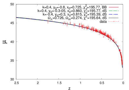
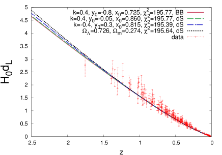
Figure 1: (Color online) The distance modulus (left panel) and dimensionless version (with $c=1$) of the luminosity distance (right panel) in recent cosmological times. The models shown here are $\Lambda$CDM (black); the tachyonic model with $k=-0.4$ evolving into de Sitter (dS, blue); tachyonic models with $k=0.4$ evolving into de Sitter (green) and into a Big Brake (BB, red).  The curves are all in very good agreement with the SNIa data, as they pass close to the local minimum of the (respective regions of the) 1-$\sigma$ domains selected by supernovae (see Figs 2 and 3 of II.)

For these specific evolutions we also show the normalized dimensionless energy density $\frac{\rho}{\rho_{cr,0}}$, pressure $\frac{p}{\rho_{cr,0}}=w\frac{\rho}{\rho_{cr,0}}$ and EoS parameter $w$ (being $w_{\mathrm{eff}}$ for the $\Lambda$CDM model) as function of the redshift (both in the past and in the future) on Figs 2-3.

Four curves appear on each graph on Figs 1-3. The black curves refer to the $\Lambda$CDM model (with value of $\Omega_{\Lambda,0}$ taken from WMAP analysis WMAP ). The dark matter component evolves here as $(1+z)^{3}$. The other three curves are for the toy model containing only the tachyon field. The three curves differ in the model parameter $k$, and in the initial data $x_{0}$, $y_{0}$. All three curves pass close to the local minimum of the respective 1-$\sigma$ domains selected by type Ia supernovae. They are characterized by the model parameter $k=-0.4$ (blue) and $k=0.4$, respectively. For the latter we have picked up both types of allowed evolutions, one going into de Sitter (green), the other ending in a Big Brake (red).

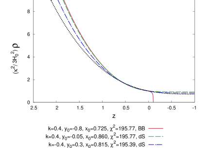
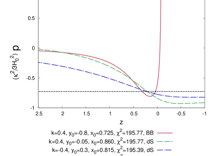
Figure 2: (Color online) The evolution in the recent past of the universe and in the future of the normalized energy density $\frac{\rho}{\rho_{cr,0}}$ (left panel) and of the normalized pressure $\frac{p}{\rho_{cr,0}}$ (right panel) is shown for four models. One of the models leads to a Big Brake singularity in the future while the other three models shown tend asymptotically to a de Sitter space.

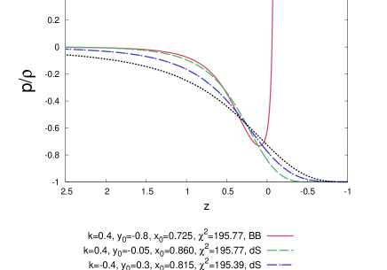
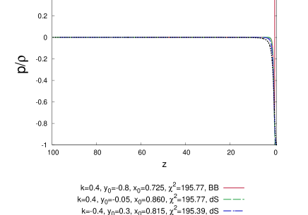
Figure 3: (Color online) The evolution of the EoS parameter $w$ ($w_{\mathrm{eff}}$ for the $\Lambda$CDM model) in the recent past and in the future is shown for the same four models, at late times from $z=2.5$ to $z=-1$ (left panel); and in the distant past from $z=100$ on (right panel). It is seen that the tachyon field behaves essentially as dustlike matter at high redshifts.

Note also that nowadays we have $w_{0}\equiv w(z=0)\in[-0.8,-0.6]$ in all the evolutions displayed. These values are similar to $\Lambda$CDM where $w_{\mathrm{eff,0}}=-\Omega_{\Lambda,0}\approx-0.74$. As expected from viable cosmological evolutions, the parameter $w$ approaches zero in the past, corresponding to dust-like behavior at early times. For all parameters, the pressure remains very slightly negative for the whole positive $z$ range plotted, thus $w$ stays below zero (although it gets very close to it). Under the assumption that this behavior is unchanged when dust is added, we expect to have a model where dark energy (here the tachyon field) remains nonnegligible in the early stages of the universe, with $\Omega_{T}$ remaining roughly constant (actually slightly increasing) during the matter era before it would start dominating at late times. A similar behavior can also be achieved in some scalar-tensor DE models, see e.g. GP08 .

II.2 Observable signature of the Big Brake?

Though the Big Brake is a singularity taking place in the future, it is interesting to investigate whether models leading to a Big Brake exhibit some signature in our present-day universe. As one can see from Fig 4, this is indeed the case for some of the universes with a Big Brake in the future which have a characteristic behavior of the EoS parameter $w$ in our past: a “dip” at low redshifts. This happens when the Big Brake is not too far in the future, in other words when the final redshift is substantially larger than $-1$. It is then interesting to investigate whether such a behavior can be detected. Actually large variations of $w$ at low redshifts can easily hide in luminosity-distance curves. Therefore, we expect that it is very difficult to observe this peculiar behavior with present SNIa data. Let us consider why this is the case in more details.

In our model we have only one component, the tachyon field, so what we call here $w$ is actually what should be called $w_{eff}$ when more fluids are present. However, it would be easy to extend our analysis to the case when a dust-like component is also present. The EoS parameter $w$ has a minimum at some small redshift $z_{min}$ with $z_{min}\sim 0.2$ in the most favorable cases. In principle this can be tested and it is straightforward to derive the following equality

$$(1+z_{min})\frac{d\ln f}{dz}\Big{|}_{z_{min}}=-1~{},$$ (16)

as well as the inequalities

$$(1+z)\frac{d\ln f}{dz} < -1~{}~{}~{}~{}~{}~{}~{}~{}~{}~{}~{}~{}~{}~{}~{}~{}~{}~{}~{}~{}~{}~{}~{}~{}~{}z<z_{min}$$ (17)

$$(1+z)\frac{d\ln f}{dz} > -1~{}~{}~{}~{}~{}~{}~{}~{}~{}~{}~{}~{}~{}~{}~{}~{}~{}~{}~{}~{}~{}~{}~{}~{}~{}z>z_{min}~{},$$ (18)

where the quantity $f$ is easily expressed in terms of the luminosity-distance, viz.

$$f=-2\frac{d}{dz}\left[\ln\left(\frac{d_{L}}{1+z}\right)^{\prime}\right]~{},$$ (19)

a prime standing for the derivative with respect to $z$.

Hence it is seen that the (in)equalities (16),(17),(18) imply a condition on the third derivative of the luminosity distance $d_{L}$! It is clear that even small uncertainties on $d_{L}(z)$ can lead to large uncertainties on its derivatives thereby rendering the (in)equalities (16),(17),(18) ineffective. In addition, as we have to apply these conditions on low redshifts, these involve third order contributions in $z$ to $d_{L}(z)$ which are inevitably small. Obviously, observational uncertainties are presently too high in order to make use of (16),(17),(18) with existing SNIa data.

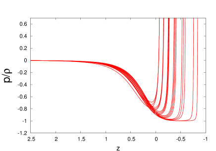
Figure 4: (Color online) The evolution of the EoS parameter $w$ in the recent past and in the future for model parameters leading to a Big Brake and in the 1-$\sigma$ domain of supernova data. All evolutions have a dip (when, as $z$ decreases, the decrease in $w$ turns into an increase), some of them already in the recent past.

Still, we have tried to see whether a standard $\chi^{2}$ analysis making use only of SNIa data in the range $0\leq z\leq z_{min}$ could differentiate models with and without dip. This means that we assume a priori that the model with the dip at $z_{min}$ is the correct one and that we investigate whether a simple statistical analysis of this relevant part of the data could hint at its presence. As could be expected, even in this case we find no statistical evidence for the detection of a dip with the present SNIa data. Note that even the Constitution dataset CfA09 contains only 147 SN data at redshifts $z\leq 0.2$. Though more refined statistical tools should clearly be used (see e.g. HPZ09 ), it is quite obvious that the present data do not allow for an unambiguous detection. Note that in some models a characteristic smoother variation of w can take place on a larger range of redshifts (see e.g. DHRS09 ) which should be easier to detect. Models involving a very large variation of $w$ at extremely low redshifts $z\ll 1$ were considered in MHH09 and it was found that they could escape all high precision measurements. In our case, variations, though not as large, are located at higher redshifts. We conjecture that future SNIa surveys, like e.g. the Large Synoptic Survey Telescope (LSST) and Wide Field InfraRed Survey Telescope (WFIRST) containing many more supernovae and reducing significantly the systematic and statistical errors could allow for such a detection. Future surveys like Euclid involving weak-lensing are also promising in this respect. We believe this could be an interesting scientific goal for these surveys especially if peculiar models with a large variation of their EoS parameter at low, but not too low, redshifts, like some of our Big Brake models with a dip, are in good agreement with observations and are theoretically motivated candidates.

III The Big Brake singularity

III.1 Curvature

The 3-spaces with $t=$const have vanishing Riemann curvature

$${}^{\left(3\right)}\mathcal{R}_{abcd}=0\,\ .$$ (20)

The 4-dimensional Riemann curvature tensor has therefore but few nonvanishing independent components:

$$R_{trtr} = -\ddot{a}a\,\ ,$$

$$R_{t\varphi t\varphi} = R_{t\theta t\theta}\sin^{2}\theta=-\ddot{a}ar^{2}\sin^{2}\theta\,\ ,$$

$$R_{r\varphi r\varphi} = R_{r\theta r\theta}\sin^{2}\theta=\dot{a}^{2}a^{2}r^{2}\sin^{2}\theta\,\ ,\,\$$

$$R_{\theta\varphi\theta\varphi} = \dot{a}^{2}a^{2}r^{4}\sin^{2}\theta\ ,$$ (21)

and the corresponding components arising from symmetry. Remarkably, all components which diverge at the Big Brake are of the type $R_{tata}$. Therefore, the singularity arises in the mixed spatio-temporal components.

III.2 Geodesic deviation

The geodesic deviation equation along the integral curves of $u=\partial/\partial t$ (which are geodesics with affine parameter $t$) is

$$\dot{u}^{a}=-R_{\ \ cbd}^{a}\eta^{b}u^{c}u^{d}\ ,$$ (22)

where $\eta^{b}$ is the deviation vector separating neighboring geodesics, chosen to satisfy $\eta^{b}u_{b}=0$. In the coordinate system (2) we obtain

$$\dot{u}^{a}=-R_{\ \ tbt}^{a}\eta^{b}\propto\ddot{a}\ ,$$ (23)

which at the Big Brake diverges as $-\infty$. Therefore, when approaching the Big Brake, the tidal forces manifest themselves as an infinite braking force stopping the further increase of the separation of geodesics. This can be also seen from the behavior of the velocity

$$v^{a}=u^{b}\nabla_{b}\eta^{a}\propto H~{},$$ (24)

which at the Big Brake vanishes. Immediately after, the negative acceleration will cause the geodesics to approach each other. Therefore a contraction phase will follow: everything that has reached the Big Brake will bounce back.

We conclude the section with the remark that despite the singularity of the geometry (the second derivative $\ddot{a}$ of the scale factor diverges at $t=t_{BB}$), its soft character ($\dot{a}$ stays regular) assures that a continuation of the evolution is still possible in the following sense. We indeed need to know $\ddot{a}$ to follow the evolution of the spacetime but we only need to know $\dot{a}$ to follow the evolution of free particles. This means that despite not being able to continue the evolution of the geometry in a direct way, we can univocally continue the individual world lines of freely falling test particles (geodesics), each of these being perfectly regular at $t=t_{BB}$. The singularity is not experienced by any individual freely falling particle, but makes itself felt only through the equation of geodesic deviation, which at $t=t_{BB}$ indicates that the expansion of the geodesic congruence turns negative from positive.

Once the particles have gone through the Big Brake, we can again start to evolve the geometry itself, thus following the further evolution of the universe beyond the singularity. As will be shown in the following section, the tachyonic universe will evolve along similar trajectories to those starting from a Big Bang, but in the opposite direction (with $s\rightarrow-s$),  arriving therefore into a Big Crunch.

IV From the Big Brake to the Big Crunch

IV.1 How the universe crosses the Big Brake singularity

To understand how the crossing of the Big Brake singularity takes place, and what is going on after the crossing, it is convenient to refer to the phase portrait of the model at some positive value of the parameter $k$. This portrait was drawn in Paper I and we reproduce it here, see Fig. 5.

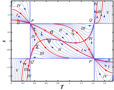
Figure 5: (Color online) Phase portrait evolution for $k>0$ ($k=0.44$)

The accessible phase space of the model consists of a rectangle $(T_{3}\leq T\leq T_{4},-1\leq s\leq 1)$ and four stripes. The values

$$T_{3}=\frac{2}{3\sqrt{(1+k)\Lambda}}\mathrm{arccos}\frac{1}{\sqrt{1+k}},$$

$$T_{4}=\frac{2}{3\sqrt{(1+k)\Lambda}}\left(\pi-\mathrm{arccos}\frac{1}{\sqrt{1+k}}\right)$$ (25)

are those for which the potential (8) vanishes. Inside the rectangle the dynamics of the system is described by the Lagrangian (1) with the potential (8), while in the strips the Lagrangian is given by

$$L=W(T)\sqrt{g^{\mu\nu}T_{,\mu}T_{,\nu}-1},$$ (26)

with the potential

$$W(T)=\frac{\Lambda}{\sin^{2}\left[\frac{3}{2}{\sqrt{\Lambda\,(1+k)}\ T}\right]}\sqrt{(1+k)\cos^{2}\left[\frac{3}{2}{\sqrt{\Lambda\,(1+k)}\,T}\right]-1}\ .$$ (27)

Consider a trajectory entering the left lower strip through the point Q’ having coordinates ($T=T_{3},s=-1$). The analysis of the equations of motion, carried out in Paper I, has shown that the universe encounters a Big Brake (BB) singularity after a finite time. This singularity is characterized by some value of the tachyon field $T_{BB}$, of the time $t_{BB}$ and of the value of the cosmological radius $a_{BB}$. These values are found numerically up to normalization, as was done in II.

The equation of motion (6) for the expanding universe in the left lower strip can be written as

$$\dot{s}=\frac{3s(s^{2}-1)\sqrt{\Lambda}}{\sin\frac{3\sqrt{\Lambda(1+k)}T}{2}}\left(\frac{(k+1)\cos^{2}\frac{3\sqrt{\Lambda(1+k)}T}{2}-1}{s^{2}-1}\right)^{1/4}$$

$$-\frac{3\sqrt{\Lambda(1+k)}(s^{2}-1)}{2}\cot\frac{3\sqrt{\Lambda(1+k)}T}{2}$$

$$\times\frac{(k+1)\cos^{2}\frac{3\sqrt{\Lambda(1+k)}T}{2}+(k-1)}{(k+1)\cos^{2}\frac{3\sqrt{\Lambda(1+k)}T}{2}-1}.$$ (28)

¿From the analysis of this equation we find that, approaching the Big Brake singularity in the lower left strip of the phase diagram, the tachyon field $T$, its time derivative $s$, the cosmological radius $a$, its time derivative $\dot{a}$ and the Hubble variable $H$ behave respectively as

$$T=T_{BB}+\left(\frac{4}{3W(T_{BB})}\right)^{1/3}(t_{BB}-t)^{1/3},$$ (29)

$$s=-\left(\frac{4}{81W(T_{BB})}\right)^{1/3}(t_{BB}-t)^{-2/3},$$ (30)

$$a=a_{BB}-\frac{3}{4}a_{BB}\left(\frac{9W^{2}(T_{BB})}{2}\right)^{1/3}(t_{BB}-t)^{4/3},$$ (31)

$$\dot{a}=a_{BB}\left(\frac{9W^{2}(T_{BB})}{2}\right)^{1/3}(t_{BB}-t)^{1/3},$$ (32)

$$H=\left(\frac{9W^{2}(T_{BB})}{2}\right)^{1/3}(t_{BB}-t)^{1/3}.$$ (33)

To arrive to formulae (29)–(33) we have used the following strategy. Assume that in the neighborhood of the Big Brake singularity the tachyon field behaves as

$$T=T_{BB}+A(t_{BB}-t)^{\alpha},$$ (34)

where $A$ and $\alpha$ are some real parameters to be determined. Then, $s$ behaves as

$$s=-\alpha A(t_{BB}-t)^{\alpha-1},$$ (35)

while its time derivative is

$$\dot{s}=\alpha(\alpha-1)A(t_{BB}-t)^{\alpha-2}.$$ (36)

A simple calculation shows that the first “friction” term, proportional to the Hubble variable in the right-hand side of Eq. (28), has the behavior

$$s^{5/2}\sim(t_{BB}-t)^{5(\alpha-1)/2},$$ (37)

which is stronger than the corresponding behavior of the second potential term in the right-hand side of Eq. (28) which is

$$s^{2}\sim(t_{BB}-t)^{2(\alpha-1)}.$$ (38)

This means that the term $\dot{s}$ in the left-hind side of Eq. (28) should have the same asymptotic as the friction term in the right-hand side of the same equation and, hence

$$\alpha-2=\frac{5}{2}(\alpha-1),$$ (39)

which gives immediately

$$\alpha=\frac{1}{3}.$$ (40)

Comparing the coefficients of the leading terms in Eq. (28) we find that

$$A=\left(\frac{4}{3W(T_{BB})}\right).$$ (41)

Thus, we arrive at Eq. (29). Eq. (30) follows right away. Using the Friedmann equation we obtain the value of the Hubble parameter (Eq. (33)), which, in turn, gives formulae (31) and (32) for the cosmological radius and for its time derivative.

The expressions (29)–(33) can be continued in the region where $t>t_{BB}$, which amounts to crossing the Big Brake singularity. Only the expression for $s$ is singular at $t=t_{BB}$, but this singularity is integrable and not dangerous.

Upon reaching the Big Brake, it is impossible for the system to stop there because the infinite deceleration eventually leads to the decrease of the scale factor. This is because after the Big Brake crossing the time derivative of the cosmological radius (32) and of the Hubble variable (33) change their signs. The expansion is then followed by a contraction.

Corresponding to given initial conditions, we can find numerically the values of $T_{BB}$, $t_{BB}$ and $a_{BB}$ (see Paper II). Then, in order to see what happens after the Big Brake crossing, we can choose as initial conditions for the “after-Big-Brake-contraction phase” some value $t=t_{BB}+\varepsilon$ and the corresponding expressions for $T,s,H,a$ and $\dot{a}$ following from relations (29)–(33), and integrate numerically the equations of motion, thus arriving eventually to a Big Crunch singularity.

IV.2 What is going on after the Big Brake crossing ?

After the Big Brake crossing the universe has a negative value of the variable $s$, less than $-1$. This means that its evolution should end in a finite period of time. Remember that the universe is now squeezing. The equation of motion for $s$ then looks as follows:

$$\dot{s}=-\frac{3s(s^{2}-1)\sqrt{\Lambda}}{\sin\frac{3\sqrt{\Lambda(1+k)}T}{2}}\left(\frac{(k+1)\cos^{2}\frac{3\sqrt{\Lambda(1+k)}T}{2}-1}{s^{2}-1}\right)^{1/4}$$

$$-\frac{3\sqrt{\Lambda(1+k)}(s^{2}-1)}{2}\cot\frac{3\sqrt{\Lambda(1+k)}T}{2}$$

$$\times\frac{(k+1)\cos^{2}\frac{3\sqrt{\Lambda(1+k)}T}{2}+(k-1)}{(k+1)\cos^{2}\frac{3\sqrt{\Lambda(1+k)}T}{2}-1}.$$ (42)

In principle, the evolution of the universe can either end at the vertical line $T=0$ at some value of $s$ or at the horizontal line $s=-1$ at some value of $T$. One can find the corresponding points on the phase diagram by direct analysis of the system of equations of motion. However, such an analysis is rather cumbersome. Thus it is convenient to use some results of the analysis of the trajectories for the expanding universe given in Paper I. Begin by writing down the equation for the trajectories describing the expanding universe in the phase space ($T,s$), eliminating the time parameter $t$:

$$\frac{ds}{dT}=-\frac{3(1-s^{2})\sqrt{\Lambda}}{\sin\frac{3\sqrt{\Lambda(1+k)}T}{2}}\left(\frac{1-(k+1)\cos^{2}\frac{3\sqrt{\Lambda(1+k)}T}{2}}{1-s^{2}}\right)^{1/4}+$$

$$-\frac{3\sqrt{\Lambda(1+k)}}{2}\frac{1-s^{2}}{s}\cot\left(\frac{3\sqrt{\Lambda(1+k)}T}{2}\right)\frac{(k+1)\cos^{2}\frac{3\sqrt{\Lambda(1+k)}T}{2}+(k-1)}{1-(k+1)\cos^{2}\frac{3\sqrt{\Lambda(1+k)}T}{2}}.$$ (43)

This equation is valid in both the rectangle of the phase diagram and in the strips. In I we have considered it in the upper left strip and saw there that the trajectories of the phase diagram can have their beginning only in the points $(T=0,s=\sqrt{\frac{k+1}{k}})$, $(T=0,s=\sqrt{k+1})$ or $(T=T_{\ast},s=1),0<T_{\ast}<T_{3}$. Now, it is easy to see from Eq. (6) that the simultaneous change of sign of the Hubble parameter $\dot{a}/a$ and of the time derivative of the tachyon field leaves this equation invariant. This means that the trajectories describing the expansion from the Big Bang singularity in the upper left strip are symmetrical reflections with respect to the axis $s=0$ of the trajectories describing the contraction towards the Big Crunch singularity in the lower left strip. Thus, equation (43) written above describes also the trajectories of the contracting universe in the lower left strip. In turn, this implies that all the contracting trajectories can only end at the points $(T=0,s=-\sqrt{\frac{k+1}{k}})$, $(T=0,s=-\sqrt{k+1})$ or $(T=T_{\ast},s=-1),0<T_{\ast}<T_{3}$.

We are now in a position to analyze the behavior of all these trajectories, describing the contracting universe, using the results obtained for the corresponding trajectories, born in the left upper strip, describing the expanding universe. First, all the contracting trajectories encountering the Big Crunch singularity at the point $(T=T_{\ast},s=-1)$, where $0<T_{\ast}<T_{3}$ and the unique trajectory ending in the point $(T=0,s=-\sqrt{k+1})$ enter the lower left strip from the rectangle of the phase diagram through the corner $(T=T_{3},s=-1)$ without arriving from the Big Brake singularity (indeed, they originate from the repelling de Sitter node). These trajectories are the time-reversed of the corresponding expanding trajectories, having their origin at the points $(T=T_{\ast},s=+1)$ and of the unique trajectory originating at the point $(T=0,s=+\sqrt{k+1})$, which enter into the rectangle through the point P (see Fig. 5) and which do not undergo any change of the expansion regime.

Thus, the only point where the trajectories coming from the crossing of the Big Brake singularity can end to is $(T=0,s=-\sqrt{\frac{k+1}{k}})$. Now recall (see Paper I) that the trajectories born at $(T=0,s=\sqrt{\frac{k+1}{k}})$ behave at the beginning of their evolution as

$$s\approx\sqrt{\frac{k+1}{k}}+DT^{\frac{2(1-k)}{1+k}},$$ (44)

where the parameter $D$ can take any real value. Among these, those with a sufficiently large positive value of $D$, say, $D_{sep}<D$ grow without limit and do not achieve a maximal value of the variable $s$. Instead, they approach asymptotically to the vertical line $T=T_{BB},s\rightarrow+\infty$, thus encountering a Big Brake shortly after the Big Bang (such a possibility was overlooked in I). Instead, the trajectories, for which $D<D_{sep}$ achieve some maximal value of the variable $s$ after which they turn down and enter the rectangle of the phase diagram through P. Such trajectories were described in detail in Paper I. The trajectory characterized by the critical value of the parameter $D=D_{sep}$ plays the role of separatrix between these two sets of the evolutions.

The trajectories approaching the Big Crunch at the point $(T=0,s=-\sqrt{\frac{k+1}{k}})$ behave as

$$s\approx-\sqrt{\frac{k+1}{k}}-DT^{\frac{2(1-k)}{1+k}}.$$ (45)

Those with $D>D_{sep}$ are the evolutions which underwent the Big Brake crossing in the left lower strip.

It is interesting to study the properties of the special cosmological evolution mentioned above ($D=D_{sep}$) which separates in the upper left strip the subset of trajectories attaining a maximum value of $s$ and then entering the rectangle at point P from the subset of those trajectories for which $s$ is not bounded above and which encounter the Big Brake already in the left upper strip. This separatrix is composed by two branches, one in the upper left strip and a symmetrical one in the lower left strip both having the vertical line $T=T_{3}$ as asymptote.

Table 1: Key moments in the evolution of the tachyon universes for $k=0.2$. Columns (1) and (2) report different pairs of values of the magnitudes $y_{0}$ and $x_{0}$ which are compatible with the supernovae data within 1$\sigma$ confidence level. Columns (3), (4), (5) and (6) report respectively the times $t_{\ast}$, $t_{BB}$ and $t_{BC}$ elapsing from the present to the tachyonic crossing, to the attainment of the Big Brake and to the later attainment of the Big Crunch, and the time lapse between the Big Brake and the subsequent Big Crunch. (The values of $t_{\ast}$, $t_{BB}$ and $t_{BC}$ have been calculated assuming for the Hubble parameter the value $H_{0}=73$ km/s/Mpc.)

$y_{0}$	$x_{0}$	$t_{\ast}\left(10^{9}yrs\right)$	$t_{BB}\left(10^{9}yrs\right)$	$t_{BC}\left(10^{9}yrs\right)$	$\left(t_{BC}-t_{BB}\right)$ $\left(10^{9}yrs\right)$
$-0.90$	$0.635$	$0.334$	$1.042$	$1.412$	$0.198$
$-0.85$	$0.845$	$2.377$	$3.093$	$3.300$	$0.207$
$-0.85$	$0.860$	$2.438$	$3.146$	$3.352$	$0.206$
$-0.85$	$0.875$	$2.505$	$3.206$	$3.410$	$0.204$
$-0.80$	$0.890$	$6.237$	$6.927$	$7.135$	$0.206$
$-0.80$	$0.905$	$6.663$	$7.348$	$7.554$	$0.206$
$-0.80$	$0.920$	$7.197$	$7.877$	$8.082$	$0.205$

Table 2: As in Table 1, for $k=0.4$.

$y_{0}$ $x_{0}$ $t_{\ast}\left(10^{9}yrs\right)$ $t_{BB}\left(10^{9}yrs\right)$ $t_{BC}\left(10^{9}yrs\right)$ $\left(t_{BC}-t_{BB}\right)$ $\left(10^{9}yrs\right)$ $-0.80$ $0.710$ $0.836$ $1.644$ $1.933$ $0.289$ $-0.80$ $0.725$ $0.841$ $1.629$ $1.915$ $0.286$ $-0.80$ $0.740$ $0.847$ $1.616$ $1.900$ $0.284$ $-0.75$ $0.815$ $2.153$ $2.952$ $3.247$ $0.295$ $-0.75$ $0.830$ $2.195$ $2.983$ $3.277$ $0.294$ $-0.75$ $0.845$ $2.242$ $3.020$ $3.312$ $0.292$ $-0.70$ $0.845$ $3.845$ $4.635$ $4.932$ $0.297$ $-0.70$ $0.860$ $3.964$ $4.746$ $5.043$ $0.297$ $-0.70$ $0.875$ $4.097$ $4.871$ $5.168$ $0.297$ $-0.70$ $0.890$ $4.247$ $5.015$ $5.310$ $0.295$ $-0.65$ $0.860$ $6.182$ $6.959$ $7.259$ $0.300$ $-0.65$ $0.875$ $6.473$ $7.243$ $7.540$ $0.297$ $-0.65$ $0.890$ $6.808$ $7.573$ $7.870$ $0.297$ $-0.65$ $0.905$ $7.204$ $7.963$ $8.259$ $0.296$ $-0.60$ $0.875$ $10.253$ $11.016$ $11.314$ $0.298$ $-0.60$ $0.890$ $11.108$ $11.866$ $12.163$ $0.297$ $-0.60$ $0.905$ $12.203$ $12.956$ $13.251$ $0.295$ $-0.55$ $0.875$ $19.517$ $20.274$ $20.570$ $0.296$ $-0.55$ $0.890$ $25.030$ $25.782$ $26.077$ $0.295$

Table 3: As in Table 1, for $k=0.6$.

$y_{0}$ $x_{0}$ $t_{\ast}\left(10^{9}yrs\right)$ $t_{BB}\left(10^{9}yrs\right)$ $t_{BC}\left(10^{9}yrs\right)$ $\left(t_{BC}-t_{BB}\right)$ $\left(10^{9}yrs\right)$ $-0.75$ $0.665$ $0.548$ $1.369$ $1.693$ $0.324$ $-0.70$ $0.755$ $1.434$ $2.289$ $2.624$ $0.335$ $-0.70$ $0.770$ $1.451$ $2.289$ $2.623$ $0.334$ $-0.70$ $0.785$ $1.469$ $2.292$ $2.625$ $0.333$ $-0.70$ $0.800$ $1.489$ $2.299$ $2.628$ $0.329$ $-0.65$ $0.815$ $2.561$ $3.401$ $3.740$ $0.339$ $-0.65$ $0.830$ $2.614$ $3.443$ $3.782$ $0.339$ $-0.65$ $0.845$ $2.671$ $3.490$ $3.827$ $0.337$ $-0.60$ $0.830$ $3.854$ $4.692$ $5.036$ $0.344$ $-0.60$ $0.845$ $3.960$ $4.788$ $5.131$ $0.343$ $-0.60$ $0.860$ $4.077$ $4.897$ $5.237$ $0.340$ $-0.60$ $0.875$ $4.206$ $5.018$ $5.359$ $0.341$ $-0.55$ $0.845$ $5.510$ $6.336$ $6.682$ $0.346$ $-0.55$ $0.860$ $5.711$ $6.530$ $6.875$ $0.345$ $-0.55$ $0.875$ $5.937$ $6.749$ $7.091$ $0.342$ $-0.55$ $0.890$ $6.194$ $6.999$ $7.339$ $0.340$ $-0.50$ $0.845$ $7.460$ $8.281$ $8.629$ $0.348$ $-0.50$ $0.860$ $7.803$ $8.617$ $8.963$ $0.346$ $-0.50$ $0.875$ $8.193$ $9.002$ $9.345$ $0.343$ $-0.50$ $0.890$ $8.645$ $9.447$ $9.790$ $0.343$ $-0.45$ $0.860$ $10.668$ $11.478$ $11.823$ $0.345$ $-0.45$ $0.875$ $11.370$ $12.174$ $12.519$ $0.345$ $-0.45$ $0.890$ $12.208$ $13.008$ $13.349$ $0.341$ $-0.45$ $0.905$ $13.237$ $14.033$ $14.373$ $0.340$ $-0.40$ $0.860$ $15.044$ $15.851$ $16.196$ $0.345$ $-0.40$ $0.875$ $16.471$ $17.273$ $17.615$ $0.342$ $-0.40$ $0.890$ $18.313$ $19.110$ $19.453$ $0.343$ $-0.40$ $0.905$ $20.838$ $21.631$ $21.972$ $0.341$ $-0.35$ $0.860$ $23.487$ $24.291$ $24.635$ $0.344$ $-0.35$ $0.875$ $27.874$ $28.674$ $29.016$ $0.342$ $-0.35$ $0.890$ $36.194$ $36.989$ $37.328$ $0.339$ $-0.30$ $0.845$ $43.469$ $44.276$ $44.621$ $0.345$

It encounters the Big Brake singularity at $T_{3}$ at some time moment $t=t_{BB}$. Now, analyzing Eq. (28) for this trajectory, we find that in the left neighborhood of $t=t_{BB}$ the dynamical variables behave as follows:

$$T=T_{3}-A_{0}(t_{BB}-t)^{2/7},$$ (46)

$$s=\frac{2}{7}A_{0}(t_{BB}-t)^{-5/7},$$ (47)

$$H=\left(\frac{147\sqrt{\Lambda k(k+1)}}{4A_{0}}\right)^{1/4}(t_{BB}-t)^{3/7},$$ (48)

where

$$A_{0}=\left(\frac{49}{12}\right)^{1/6}\Lambda^{-5/12}(1+k)^{-5/12}k^{1/4}.$$ (49)

The analysis leading to these formulae is analogous to the one which led us to formulae (29)–(33).

If we continue (46)–(49) beyond $t=t_{BB}$ we see that the expansion turns into a contraction, the tachyon field $T$ starting to decrease, while its time derivative jumps at $t=t_{BB}$ from an infinite positive value to an infinite negative one. Thus, at $t>t_{BB}$ the universe finds itself in the lower left strip. It leaves the Big Brake along the asymptotic line $T=T_{3},s=-\infty$, and eventually attains the Big Crunch singularity at the point $(T=0,s=-\sqrt{\frac{k+1}{k}})$. In the lower left strip the separatrix separates the trajectories exiting from the Big Brake singularity at some value $T_{BB}<T_{3}$ from those which enter the strip from the rectangle, attain a minimum value of $s$ and end in the Big Crunch.

In summary, the expansion phase of the universe, which originated from a Big Bang, stops at $t=t_{BB}$ and turns there into a phase of contraction leading eventually to a Big Crunch.

IV.3 The time lapse from the Big Brake to the Big Crunch

We give here the Tables 1-3 which, for a selection of values of the model parameter $k$, report the times elapsing from today to the tachyonic crossing, to the attainment of the Big Brake and to the later attainment of the Big Crunch for some trajectories which are compatible with SNIa data within a 1-$\sigma$ confidence level.

As we can see, although the time to the tachyonic crossing and to the Big Brake both depend strongly on the initial data within the 1-$\sigma$ domain selected by supernovae, the time interval between the Big Brake and the Big Crunch do not show the same dependence. Nevertheless, this interval exhibits a slight increase with the model parameter $k.$

V Conclusions

As shown in II there are tachyon cosmologies described by Eqs.(1)-(13) which are compatible with the supernovae data and which are subject to a Big Brake in the future. In this paper we have addressed some questions about this model: how it behaves in the distant past, whether these model universes can produce observational signatures today and whether they can be continued beyond the Big Brake singularity.

Having in mind the eventual construction of fully viable models, we are comforted by the fact that the tachyonic field has a (quasi) dust-like behavior in the past regardless of its future evolution in the parameter range allowed by supernovae. Present supernovae data can hardly discriminate between the evolutions going into a de Sitter phase and those leading to a Big Brake. However, we emphasize that the large variation of the EoS parameter at low redshifts occurring in some of the evolutions leading to a Big Brake might be detectable with future high precision data.

The main result of the paper is the study of the cosmological evolutions going into a Big Brake. These evolutions can be extended beyond the Big Brake, despite the geometry becoming singular, which apparently forbids such a continuation. However, this singularity is a soft one, as only the second derivative $\ddot{a}$ of the scale factor diverges at $t=t_{BB}$, while $\dot{a}$ does not. We need to know $\ddot{a}$ to follow the evolution of the spacetime but we only need to know $\dot{a}$ to follow the evolution of free particles. This means that we can not continue the evolution of the geometry, but we can univocally continue the individual world lines of freely falling test particles (geodesics), each of these being perfectly regular at $t=t_{BB}$. The singularity is not experienced by any individual freely falling particle, but makes itself felt only through the equation of geodesic deviation, which at $t=t_{BB}$ indicates that the expansion of the geodesic congruence turns negative from positive.

Since the geometry can be reconstructed by the knowledge of each of its geodesics, the evolution of the universe does not stop at the Big Brake. Once the particles have gone through the Big Brake, they will determine the geometry anew and we can start to evolve the universe beyond the singularity. A phase of contraction follows, leading eventually to a Big Crunch.

We have analytically and numerically analyzed the evolution of the tachyonic universe from the Big Brake to the Big Crunch. Quite remarkably, the numerical study showed that although the time to the tachyonic crossing and to the Big Brake both depend strongly on the initial data chosen from the 1-$\sigma$ domain selected by supernovae, the time intervals between the Big Brake and the Big Crunch do not exhibit the same dependence and they only slightly depend on the model parameter $k$ (within a factor of two). This seems to provide an invariant timescale for the class of tachyonic scalar cosmologies considered, presumably related to the fact that some information (the behavior of the higher derivatives of the scale factor) is lost while passing through the Big Brake.

References

- (1) A. Riess et al., Astron. J. 116, 1009 (1998); S. J. Perlmutter et al., Astroph. J. 517, 565 (1999).
- (2) S. Tsujikawa, in Dark Matter and Dark Energy: a Challenge for Cosmology, edited by S. Matarrese, M. Colpi, V. Gorini, and U. Moschella (Springer, New York, to be published).
- (3) V. Sahni and A.A. Starobinsky, Int. J. Mod. Phys. D 9, 373 (2000); 15, 2105 (2006); T. Padmanabhan, Phys. Rep. 380, 235 (2003); P.J.E. Peebles and B. Ratra, Rev. Mod. Phys. 75, 559 (2003); E.J. Copeland, M. Sami and S.Tsujikawa, Int. J. Mod. Phys. D 15, 1753 (2006).
- (4) L. Perivolaropoulos, arxiv:0811.4684.
- (5) M. Born and L. Infeld, Proc. Roy. Soc. Lond. A 144, 425 (1934).
- (6) A. Sen, JHEP 0207, 065 (2002); G.W. Gibbons, Phys. Lett. B 537, 1 (2002); A. Feinstein, Phys. Rev. D 66, 063511 (2002); T. Padmanabhan, Phys. Rev. D 66, 021301 (2002); N. Barnaby, JHEP 0407, 025 (2004); R. Herrera, D. Pavon and W. Zimdahl, Gen. Rel. Grav. 36, 2161 (2004); J. M. Aguirregabiria and R. Lazkoz, Mod. Phys. Lett. A 19, 927 (2004); A. Sen, Phys. Scripta T117, 70 (2005); E. J. Copeland, M. R. Garousi, M. Sami and S. Tsujikawa, Phys. Rev. D 71, 043003 (2005); R. Lazkoz, Int. J. Mod. Phys. D 14, 635 (2005); V. Gorini, A. Kamenshchik, U. Moschella, V. Pasquier and A. Starobinsky, Phys. Rev. D 72, 103518 (2005); E. Elizalde and J. Q. Hurtado, Int. J. Mod. Phys. D 14, 1439 (2005); C. Quercellini, M. Bruni and A. Balbi, Class. Quant. Grav. 24, 5413 (2007); J. Martin and M. Yamaguchi, Phys. Rev. D 77, 123508 (2008).
- (7) A. Frolov, L. Kofman and A. Starobinsky, Phys. Lett. B 545, 8 (2002).
- (8) V. Gorini, A.Yu. Kamenshchik, U. Moschella, and V. Pasquier, Phys. Rev. D 69, 123512 (2004).
- (9) J. D. Barrow, G. J. Galloway, and F. J. Tipler, Mon. Not. Roy. Astron. Soc. 223, 835- 844 (1986); J. D. Barrow Phys. Lett. B 235, 40-43 (1990); J. D. Barrow, Class. Quant. Grav. 21, L79 (2004); J. D. Barrow, Class. Quant. Grav. 21, 5619 (2004); J. D. Barrow, A. B. Batista, J. C. Fabris, and S. Houndjo, Phys. Rev. D 78, 123508 (2008); M. P. Dabrowski, T. Denkiewicz, and M. A. Hendry, Phys. Rev. D 75, 123524 (2007); J. D. Barrow and S. Z. W. Lip, Phys. Rev. D 80, 043518 (2009).
- (10) Z. Keresztes, L. Á. Gergely, V. Gorini, U. Moschella, A.Yu. Kamenshchik, Phys. Rev. D 79, 083504 (2009). The model parameter was denoted there by and the energy density by .
- (11) W. M. Wood-Vasey et al. [ESSENCE Collaboration], Astrophys. J. 666, 694 (2007).
- (12) L. Á. Gergely, Z. Keresztes, A. Yu. Kamenshchik, V. Gorini, U. Moschella, AIP Conf. Proc. 1241, 884 (2010).
- (13) L. Fernández-Jambrina, R. Lazkoz, Phys. Rev. D 70, 121503(R) (2004).
- (14) A. Balcerzak, M. P. Dabrowski, Phys. Rev. D 73, 101301(R) (2006).
- (15) E. Komatsu, J. Dunkley, M. R. Nolta at al., Astrophys. J. Suppl. 180 330 (2009)
- (16) R. Gannouji, D. Polarski JCAP 0805, 018 (2008).
- (17) M. Hicken et. al., Astrophys. J. 700 1097 (2009).
- (18) Hojjati, L. Pogosian, Gong-Bo Zhao, JCAP 1004, 007 (2010).
- (19) M. Mortonson, W. Hu, D. Huterer, Phys. Rev. D 80, 067301 (2009).
- (20) S. Dutta, S.D.H. Hsu, D. Reeb, R. J. Scherrer, Phys. Rev. D 79 103504 (2009).