Isentropic Curves at Magnetic Phase Transitions

Abstract

Experiments on cold atom systems in which a lattice potential is ramped up on a confined cloud have raised intriguing questions about how the temperature varies along isentropic curves, and how these curves intersect features in the phase diagram. In this paper, we study the isentropic curves of two models of magnetic phase transitions- the classical Blume-Capel Model (BCM) and the Fermi Hubbard Model (FHM). Both Mean Field Theory (MFT) and Monte Carlo (MC) methods are used. The isentropic curves of the BCM generally run parallel to the phase boundary in the Ising regime of low vacancy density, but intersect the phase boundary when the magnetic transition is mainly driven by a proliferation of vacancies. Adiabatic heating occurs in moving away from the phase boundary. The isentropes of the half-filled FHM have a relatively simple structure, running parallel to the temperature axis in the paramagnetic phase, and then curving upwards as the antiferromagnetic transition occurs. However, in the doped case, where two magnetic phase boundaries are crossed, the isentrope topology is considerably more complex.

I. Introduction

In systems of interacting degrees of freedom, decreasing the thermal fluctuations often leads to the formation of ordered states. The traditional, and natural, measure of these fluctuations is the temperature $T$ itself, which then forms one axis of the associated phase diagrams. However entropy $S$ can also be used to quantify the amount of disorder. Indeed, a phase diagram using $S$ as an axis naturally provides a somewhat different perspective on the topology of the ordered and disordered regions- since the entropy changes more rapidly where transitions occur, it magnifies these interesting portions of the phase diagram.

Recent experimentsjaksch98 ; greiner02 ; bloch04 ; lewenstein07 on trapped ultracold atoms in optical lattices have provided a further motivation for employing the entropy as one of the variables in describing phase diagrams.optlatS ; optlatS2 In these systems, the temperature and entropy of the atomic cloud are known prior to the adiabatic ramp-up of the optical lattice, but the precise change in temperature during this process is uncertain. Thus the determination of the entropy values at which various phenomena occur, like local moment formation, magnetic ordering, and so forth, is important, supplementing the more typical discussion of the temperatures at which these phenomena occur. Furthermore, since attaining low temperatures is crucial for the emulation of many-body ordering effects seen in solid state systems, a central question is whether $T$ rises or falls (adiabatic heating or cooling) as the optical lattice is established.

This work examines the isentropic curves of two models of magnetic phase transitions. The two-dimensional Blume-Capel Model (BCM)blume66 ; capel66 is studied first, and its thermodynamics are computed both in Mean Field Theory (MFT) and with Monte Carlo (MC) methods. An itinerant (quantum) Hamiltonian, the Fermion Hubbard Model (FHM) is next examined within MFT. The isentropes of the FHM are compared with recent Quantum Monte Carlo (QMC)paiva10 results at half-filling, a density at which QMC can be performed to low temperatures. The isentropes are also computed when the system is doped away from half-filling, a parameter regime where phases with long range order are inaccessible to QMC. The BCM and FHM form an interesting pair of models to compare, since both contain two energy scales, one which controls the density and the other which tunes the strength of spin-spin interactions.

The paper is organized as follows: Sec. II presents both the BCM and the FHM, and the computational methods used. Sec. III then details the isentropes of the BCM, while Sec. IV focused on the FHM. Sec. V summarizes and further discusses the results.

II. Models and Computational Approach

.1 Blume Capel Model

The Blume-Capel Modelblume66 ; capel66 is,

$$E=-J\sum_{\langle{\bf ij}\rangle}S_{\bf i}S_{\bf j}+D\sum_{\bf i}S_{\bf i}^{2}\,\,.$$ (1)

The spins $S_{\bf i}$ can take three values $S_{\bf i}=0,\pm 1$, where the value $S_{\bf i}=0$ can be regarded as a ‘vacancy’. The first term in the energy represents a ferromagnetic coupling $J$ between near-neighbor spins. The second term provides an ’impurity’ chemical potential $D$ for the vacancies. When $D$ is large and negative, vacancies are suppressed, and the BCM maps onto the Ising model. Here we will consider a square lattice geometry.

The presence of a three component spin gives rise to the possibility of first order transitions and tricritical behavior, as first emphasized in [griffiths73, ]. Part of the original motivation for the BCM was to provide a description of the tricritical phenomena induced by ³He vacancies in superfluid ⁴He.graf67 ; goellner71 ; ahlers74 Since its introduction, the BCM has been extensively studied,berker76 ; burkhardt77 ; saul74 ; jain80 ; wang87 ; hoston91 ; beale86 ; rachadi03 both in the form given in Eq. 1, and in several variants which include additional terms in the energyblume71 ; mukamel74 and generalizations to vector spins which more correctly capture the continuous symmetry of the superfluid order parameter.cardy79 ; berker79 ; chamati07 ; dillon10

The solution of the BCM within MFT is straightforward. The results for the free energy and entropy (per site) are,

$$f = \left(\frac{Jzm^{2}}{2}\right)-\frac{1}{\beta}\ln\ [2\cosh(\beta Jzm)+e^{\beta D}]+D$$ (2)

$$s = -\beta[Jzm^{2}+(1-\rho)D]+\ln[2\cosh(\beta Jzm)+e^{\beta D}]$$

where z is the coordination number ($z=4$ for square lattice). The magnetization $m$ and density of spin states $\rho$ are given by the self-consistency equations:

$$m = \frac{2\sinh(\beta Jmz)}{e^{\beta D}+2\cosh(\beta Jmz)}$$

$$\rho = \frac{2\cosh(\beta Jmz)}{e^{\beta D}+2\cosh(\beta Jmz)}$$ (3)

Here we set $J=1$ as a unit of energy, and solve Eqs. 2,3 to obtain the free energy and entropy for any values of independent variables D and $\beta$ .

We compared two different MC approaches for computing entropy in the BCM: thermodynamic integration and the Wang-Landau (WL) algorithm. With thermodynamic integration, the entropy is computed by making multiple MC runs at different, fixed inverse temperatures $\beta$ and integrating,

$$s(\beta)=s(\infty)+\beta e-\int_{\beta}^{\infty}e(\beta)d\beta\,\,,$$ (4)

where $s$ and $e$ are the entropy and energy per site, respectively. Equation 4 is obtained by applying integration by partsbinder81 ; tremblay07 ; paiva10 to the standard relation of entropy to the specific heat: $S(T)=\int_{0}^{T}C(T^{\prime})/T^{\prime}\,dT^{\prime}$. For the BCM, $s(\infty)=\ln 3$, reflecting the three possible choices of spin. In most instances, this approach produces better results, since it does not rely on the determination of specific heat $C(T)$, which is noisier than the energy $e(T)$.

The WL algorithm is a flat-histogram MC method for calculating the density of states $g(E)$. In this method, a random walk is performed in the energy space of the BCM, sampling $E$ with a probability proportional to $1/g(E)$ and adjusting the distribution of $g(E)$ until each energy (E) value has close to the same probability. Ultimately, this process produces a flat histogram of occurrence for all energy states in the random walk. Since the density of energy states that results is independent of temperature, we can compute the partition function $Z=\sum_{E}g(E)e^{-\beta E}$ for any temperature. Consequently, we can determine the value for any thermodynamic variable of interest- in our case, the free energy and entropy- without performing multiple MC simulations at different $\beta$.

Figures and analysis reported for BCM will be those from WL results on 16x16 lattices. The values obtained for the entropy with the two methods, however, were found to be equivalent to within a fraction of a percent.

.2 Hubbard Hamiltonian

The Fermion Hubbard Model,hubbard63

$$H= - t\sum_{\langle{\bf ij}\rangle\,\sigma}(c_{{\bf i}\sigma}^{\dagger}c_{{\bf j}\sigma}^{\vphantom{dagger}}+c_{{\bf j}\sigma}^{\dagger}c_{{\bf i}\sigma}^{\vphantom{dagger}})$$ (5)

$$+ U\sum_{{\bf i}}n_{{\bf i}\uparrow}n_{{\bf i}\downarrow}-\mu\sum_{{\bf i}\sigma}n_{{\bf i}\sigma}\,\,,$$

describes the magnetism of itinerant electrons, in contrast to the static spins of the Blume-Capel model. Here $c_{{\bf i}\sigma}^{\dagger}(c_{{\bf i}\sigma}^{\vphantom{dagger}})$ are creation(destruction) operators for fermions of spin $\sigma$ on lattice site ${\bf i}$, and $n_{{\bf i}\sigma}$ are the associated number operators. $t=1$ sets the kinetic energy scale for the hopping of fermions between near neighbor sites of a square lattice. $U$ is an on-site energy cost for double occupancy, and the chemical potential $\mu$ controls the filling.

One interesting property of the square lattice, near-neighbor hopping is that the associated dispersion relation $\epsilon(k_{x},k_{y})=-2t[{\rm cos}k_{x}+{\rm cos}k_{y}]$ has a (logarithmic) divergent density of states at half-filling. As a consequence, the Stoner criterion suggests that an arbitrarily small interaction $U$ will induce a magnetic instability. This is reflected in the phase diagrams shown in Figs. 5 and 6.

The FHM has been widely used to study strong correlation effects in solids, from magnetism to metal-(Mott) insulator transitions, and high temperature superconductivity.hubbard63 ; rasetti91 ; montorsi92 ; fazekas99 Recently, the FHM and its bosonic counterpart have attracted considerable interest for describing the behavior of cold atoms trapped in an optical lattice produced by interfering laser beams.jaksch98 Compared with traditional condensed matter experiments, these optical lattice systems are thought to more precisely mimic the FHM, while allowing tunable control over parameters like $U$ and $t$. As mentioned in the introduction, this provides a central motivation for this paper.

Our MFT approach is the usual one in which each term of the interaction is decoupled: $Un_{{\bf i}\uparrow}n_{{\bf i}\downarrow}\rightarrow Un_{{\bf i}\uparrow}\langle n_{{\bf i}\downarrow}\rangle+U\langle n_{{\bf i}\uparrow}\rangle n_{{\bf i}\downarrow}-U\langle n_{{\bf i}\uparrow}\rangle\langle n_{{\bf i}\downarrow}\rangle$. The resulting quadratic Hamiltonians $H_{\sigma}$ are diagonalized, and the expectation values $\langle n_{{\bf i}\sigma}\rangle$ recomputed. The process is iterated to self-consistency, a process which minimizes the free energy $F$. To be somewhat more precise, the MFT calculation is actually performed in momentum space by making particular, simple, paramagnetic (P), ferromagnetic (F), and antiferromagnetic (AF) ansatz for the real space expectation values $\langle n_{{\bf i}\sigma}\rangle$. Such a choice does not allow for more complex spatial patterns of charge and spin such as are present in striped phases.zaanen89

Our results for the isentropic curves of the FHM will be obtained exclusively within MFT. It is possible to obtain these curves using more exact approaches like QMC,paiva10 but only in parameter regimes like half-filling where there is no sign problem.Previous Dynamical Mean Field Theory work has also reported data for the isentropes on a cubic lattice.werner05 ; optlatS2

III. Isentropic Curves of the Blume-Capel Model

Single Site Limit

We begin our analysis of the isentropic curves by discussing the $J=0$ limit of a collection of independent spin-1 sites. The partition function is,

$$Z=1+2e^{-\beta D}\,\,,$$ (6)

from which we can derive the internal energy, free energy, and entropy,

$$\langle E\rangle = Z^{-1}2De^{-\beta D}$$

$$F = -\frac{1}{\beta}\,{\rm ln}\,Z$$

$$S = \beta(\langle E\rangle-F)\,\,.$$ (7)

Since only the combination $\beta D$ enters the expressions in Eq. 7, the isentropic condition, $S=S_{0}$ implies that $\beta D=c$, where the constant $c$ is obtained by solving the transcendental equation,

$$S_{0}=\frac{2c\,e^{-c}}{1+2e^{-c}}+\ln(1+2e^{-c})\,\,.$$ (8)

We immediately see that the isentropic curves are straight lines $D=cT$. Note that for values of $S_{0}$ greater than $\ln 2\sim.693$, there are two solutions for $c=D/T$, one positive and one negative, representing positive and negative values of $D$. In this single site limit, values of $D$ less than zero will suppress all vacancies, preventing entropy values less than $\ln 2$.

Despite the simple nature of this calculation, it allows us to make some immediate statements about adiabatic heating and cooling. We see that in traveling along an isentrope of increasing $D$ from $D=-\infty$, the temperature $T$ decreases, since one moves along a line with $c<0$. Ultimately, one reaches $D=0$ where the sign of $c$ changes to positive, and further movement along the isentrope results in an increase in temperature.

The interesting question is, of course, how the topology of the isentropes of the noninteracting systems is altered by interactions and, in particular by the strong collective effects which occur near the magnetic phase boundary.

Mean Field Theory

Having discussed the $J=0$ limit, we now address the isentropic curves of the BCM treated within MFT. Solving the self-consistency Eq 3, we show the resulting isentropes in Fig. 1 along with the mean-field phase boundary (PB). The PB consists of a first order line (shown in full red) and second order boundary (dashed green), which meet at the tricritical point (TP): $(T_{\rm tp},D_{\rm tp})=(\frac{4}{3},\frac{8}{3}\ln 2)$. The TP and second order PB can be obtained analytically by expanding the free energy in powers of the magnetization $m$ and computing the Landau coefficient for the $m^{2}$ term, thus fixing the transition line. (See Ref. [blume66, ].)

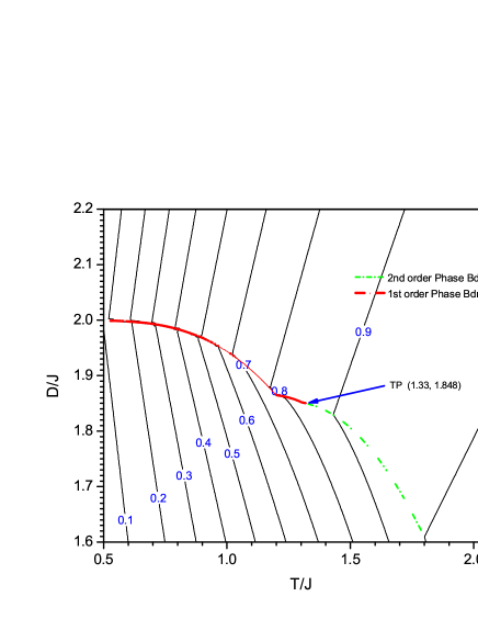
Figure 1: (color online). Mean-Field Theory calculation of the isentropes of the Blume-Capel model. The temperature $T$ decreases as $D$ increases along the isentropes in the ordered phase, and then rises in the paramagnetic phase. $S$ jumps at the phase boundary below the tricritical point, and is continuous above.

At the first order phase boundary, the entropy shows a characteristic “jump,” or discontinuity, as the isentropes take a sharp jog to the left (smaller $T$) in passing through the boundary (Fig. 1). The entropy decreases in this traversal of the PB to higher $D$ values at fixed $T$ due to the large reduction in the spin density $\rho$. Below the PB in the ferromagnetic phase (F), spin-0 “vacancies” are sparse, resulting in an effective (Ising-like) two spin state region and lower entropy. Above the PB, all three spin states are present with higher entropy.

In contrast, at the second order boundary (dashed green line in Fig. 1), the isentropes are continuous, but exhibit a change in slope at the PB. As we will see shortly, the precise details of this behavior are peculiar to the MFT and do not carry over to the exact (MC) solutions which incorporate short range correlations and fluctuations. Nevertheless the general topology of the isentropes in MFT agree with those of MC.

Monte Carlo- Wang-Landau

The phase diagram of the BCM was determined by first using the WL density of states to compute thermodynamic variables, the free energy $f$, entropy $s$, specific heat $C(T)$, and magnetic susceptibility $\chi(T)$, for a fine grid of points in the ($D$,$T$)-plane. We then examined specific conditions to locate the phase transition points. For 1st order transitions, we looked for jumps in the entropy coinciding with a vanishing magnetic order parameter ($m$). For 2nd order transitions, we located peaks in specific heat and magnetic susceptibility curves plotted as a function of temperature for fixed $D$.

Representative results are shown in Fig. 2. Here $C(T)$ is obtained for fixed impurity chemical potentials $D=0.0,0.5,1.0,$ and $1.5$. Peaks are observed at temperatures which are associated with the large fluctuations at the second order phase transition. Finite size scaling, and other sophisticated techniques can be exploited to locate $T_{c}$ very precisely. For example, as $D$ is increased further, it is known that a tricritical point exists in the BCM at $(T_{\rm tp},D_{\rm tp})=(.610,1.965)$. This change in behavior can be seen numerically by monitoring, the appearance of hysteresis loops when MC simulations are done sweeping $D$ at fixed $T<T_{\rm tp}$.

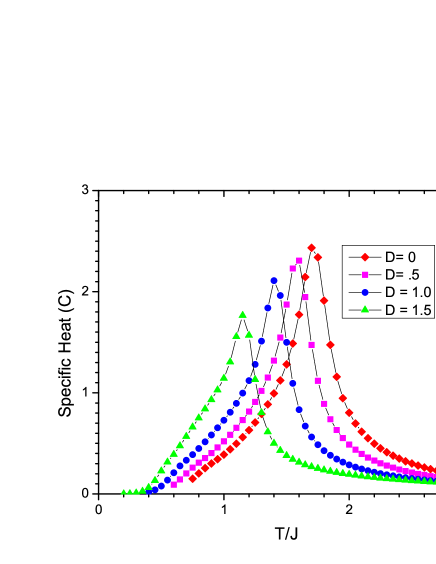
Figure 2: (color online). Wang-Landau MC results for the specific Heat $C(T)$ for different values of the vacancy chemical potential $D=0.0,0.5,1.0,1.5$ in the second order phase transition region. The peak positions give one estimate of the phase boundary.

Plots like that of Fig. 2 for different values of $D$, as well as sweeps in $D$ at fixed $T$, were used to locate the phase transition line in the $T-D$ plane. This is shown as the black dashed line in Fig. 4. The phase boundary thus obtained is in good agreement (less than a percent difference) with published results. The new aspect of Fig. 4 is the inclusion of the isentropic curves.

The gross linear structure of the isentropes for large $T/J$ and $D/J$ is well explained by the $J=0$ (single site) analysis earlier in this section. However, at intermediate $T/J$ and $D/J$, the isentropes are rounded, especially in the vicinity of the phase boundary. Indeed, the boundary between adiabatic heating and cooling does not precisely follow the PB but instead occurs along a separate trajectory of somewhat larger impurity chemical potential.

As discussed in [mahmud10, ], the key qualitative feature of the isentropes is that they move out to higher $T$ as they leave either side of the phase boundary (into the paramagnetic or ferromagnetic phases). The simple picture of this result is that the boundary represents a line of a high degree of competition between different phases, and hence a high entropy $S$. In order for $S$ to remain constant as we move away from the boundary, the temperature must increase. If an experiment were performed in which $D$ were ramped, the lattice would cool as the phase boundary is approached from the ferromagnetic side, and heat as one moves away into the paramagnet.

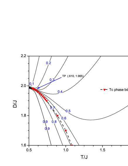
Figure 3: (color online). Wang-Landau MC results for the spin density contours of the Blume-Capel model. The vacancy density increases as the temperature $T$ or chemical potential $D$ rise. Ferromagnetic order is lost when roughly one third of the sites are vacant.

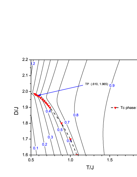
Figure 4: (color online). Wang-Landau MC results for the isentropes of the Blume-Capel model. As for the MFT calculation, the isentropes exhibit adiabatic cooling in the ferromagnetic phase, and heating in the paramagnetic phase. The entropy curves become discontinuous at the tricritical point.

Comparing the isentrope contours, Fig. 4, with the those for spin density as shown in Fig. 3, we see that as we traverse the first order phase boundary, the spin density changes more rapidly as the temperature $T$ approaches zero. In fact, this is consistent with Clausius-Clapeyron equation which relates the slope of the phase boundary with the change in entropy and spin density by,

$$\frac{dD}{dT}=-\frac{s_{\rm fm}-s_{\rm pm}}{\rho_{\rm fm}-\rho_{\rm pm}}$$ (9)

where $s_{\rm fm}$ and $s_{\rm pm}$ stand for entropy in the ferromagnetic and paramagnetic phases respectively. We have verified that our results satisfy this condition quantitatively.

IV. Isentropic Curves of the Hubbard Hamiltonian

We now turn to the isentropic curves of the Hubbard Hamiltonian. The ground state MFT phase diagram is shown in Fig. 5, and consists of paramagnetic $P$ regions adjacent to empty and fully occupied fillings ($\rho=0,2$). In the center, closer to half-filling, magnetic phases arise, with antiferromagnetism AF predominating immediately adjacent to $\rho=1$ and ferromagnetism F a bit farther away, at sufficiently large $U$. The phase diagram is symmetric about $\rho=1$, as a consequence of the particle-hole symmetry of the Hubbard model on a bipartite lattice with near-neighbor hopping.

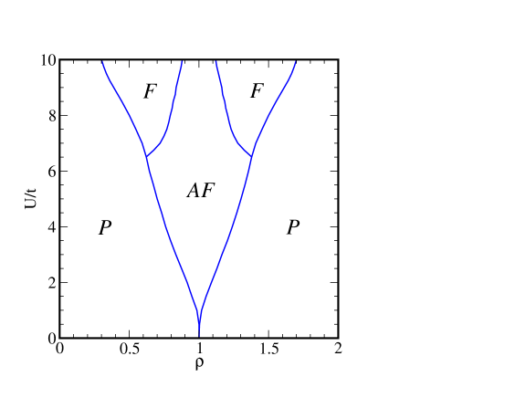
Figure 5: (color online). Ground state MFT phase diagram of the two dimensional square lattice Hubbard model. Antiferromagnetism is favored at and near half-filling, and extends all the way to $U=0$ as a consequence of the divergence of the $\rho=1$ density of states. Ferromagnetic regions are present at stronger coupling.

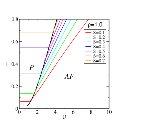
Figure 6: (color online). Isentropic curves of the half-filled square lattice Hubbard model. $S$ is independent of $U$ in the paramagnetic phase. The isentropic curves are continuous and bend upwards upon entering the ordered antiferromagnetic region. The entire $T=0$ axis is AF. (See text and Fig. 5.)

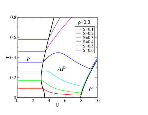
Figure 7: (color online). Isentropic curves of the square lattice Hubbard model at density $\rho=0.8$. As at $\rho=1.0$ (Fig. 6), $S$ is independent of $U$ in the paramagnetic phase. The isentropic curves are continuous upwards upon entering the ordered antiferromagnetic region, trending upwards for large $S$ and downwards for small $S$. The isentropic curves are discontinuous at the AF $\rightarrow$ F transition. As $U$ is increased at $T=0$, there is first a P $\rightarrow$ AF transition, followed by a AF $\rightarrow$ F transition. (See text and Fig. 5.)

Figure 6 shows the phase boundary in the $T/t-U/t$ plane at half-filling $\rho=1$. As discussed earlier, the associated isentropes are parallel to the $U/t$ axis in the paramagnetic phase. They then bend to higher $T/t$ as $U/t$ increases in the antiferromagnet. This adiabatic heating is explained by the same reasoning as for the classical BCM case: The phase boundary represents a location of particularly high entropy, so that for $S$ to remain fixed as one leaves its vicinity the temperature must increase. The gross morphology for the isentropes found in Fig. 6 agrees well with exact QMC calculationspaiva10 which can be performed with no sign problem in this half-filled case. The QMC method, which is exact, of course captures the fact that there is no finite temperature phase transition in the square lattice FHM. The role of the phase boundary there is played by the temperature scale of the mean field charge gap, which is determined by the plateau in $\rho$ versus $\mu$.

Figure 7 shows the analogous phase boundaries and isentropes for $\rho=0.8$. Here the structure is much richer since there are three possible phases for this density, with the paramagnet first giving way to antiferromagnetic order as $U/t$ is increased, followed by a second transition to ferromagnetism. In this case the isentropes can bend either to higher or to lower $T$ as the AF boundary is left with increasing $U$. The decrease in $T$ occurs at lower $T/t$ where the F boundary is more proximate to the AF one. The isentropes move to higher $T$ as $U/t$ decreases from the F phase boundary. The other interesting feature of Fig. 7, not present in Fig. 6, is the discontinuity in the isentropes at the AF-F boundary. This occurs here, similar to the situation for temperatures below the tricritical point in the BCM model, because of the first-order nature of the transition. As with the BCM, we have verified that the entropy jump along the first order boundary satisfies the Clausius-Clapeyron relation, which here takes the form,

$$\frac{dU}{dT}=\frac{s_{\rm fm}-s_{\rm afm}}{{\cal D}_{\rm fm}-{\cal D}_{\rm afm}}\,\,.$$ (10)

Here $\frac{dU}{dT}$ is the slope of the AF-F phase boundary, $s_{\rm fm},s_{\rm afm}$ are the associated entropies, and ${{\cal D}_{\rm fm},{\cal D}_{\rm afm}}$ are the double occupations in the two phases.

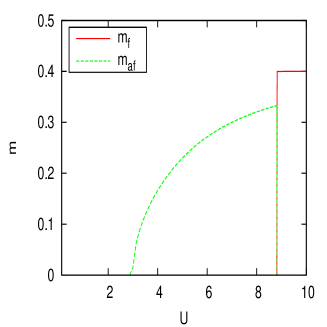
Figure 8: (color online). The antiferro- and ferro-magnetic order parameters are shown for $\rho=0.8$ and $T=0.2$. As $U$ increases from zero there is a continuous transition to an AF phase followed by a discontinuous transition to a F phase.

The behavior of the ferromagnetic, $m_{\rm f}$, and antiferromagnetic, $m_{\rm af}$, order parameters for $\rho=0.8$ and $T=0.2$ is shown in Fig. 8. Both change discontinuously through the first order AF-F transition at $U\approx 8.8t$. However at the second order P-AF transition at $U\approx 3t$, $\,m_{\rm af}$ increases continuously from zero with the MFT exponent $\beta=\frac{1}{2}$.

An interesting feature of the P $\rightarrow$ AF phase boundary at $\rho=0.8$ is that the critical $U$ initially decreases as the temperature $T$ increases. Put another way, as $T$ is lowered for $U\approx 3.2$ there is a P $\rightarrow$ AF ordering transition, but then there is a re-entrance to the P phase as $T$ is reduced further. We have verified that this phenomenon is obtained also within an independent random phase approximation calculation, in which the magnetic susceptibility is given by,

$$\chi({\bf q},T) = \frac{\chi_{0}({\bf q},T)}{1-U\chi_{0}({\bf q},T)}$$

$$\chi_{0}({\bf q},T) = \sum_{\bf k}\frac{f(\epsilon_{{\bf k}+{\bf q}})-f(\epsilon_{{\bf k}})}{\epsilon_{{\bf k}}-\epsilon_{{\bf k}+{\bf q}}}\,\,.$$ (11)

The critical temperature is then determined from Eq. 11 via the Stoner criterion $1-U\chi_{0}({\bf q},T)=0$, and exhibits the same re-entrant phenomenon as the MFT calculation.

Finally, we show in Fig. 9 the phase diagram and isentropes for quarter filling. At zero temperature (see Fig. 5) there is a paramagnetic to ferromagnetic transition as $U$ increases. However, at higher $T$ an intermediate antiferromagnetic phase intervenes. The general trend is towards adiabatic heating as $U$ rises.

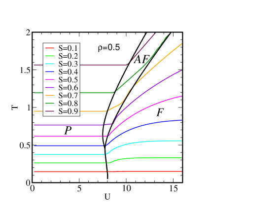
Figure 9: (color online). Phase diagram and isentropes for quarter filling. For $T>0.5t$, an antiferromagnetic region appears between the paramagnetic region at weak coupling and ferromagnetic region at strong coupling.

V. Conclusions

In this paper, the isentropic curves of a classical system of magnetism, the Blume-Capel model, and of the quantum fermion Hubbard Hamiltonian, have been determined.

In the case of the BCM, Mean Field Theory and Monte Carlo (Wang-Landau) calculations give a qualitatively similar pictures in which adiabatic heating is observed as one moves away from the phase boundary, although the precise, quantitative location of the transition is, of course, different in the two methods. The behavior of the isentropes is made somewhat more complex by the presence of a tricritical point on the BCM phase boundary, so that there is a region at low $T$ and large vacancy fraction where the curves are discontinuous.

For the FHM, we have presented only MFT results, since the sign problem in general prevents Quantum Monte Carlo simulations at low temperatures. The topology of the isentropes, like the phase diagram itself, is relatively simple at half-filling, consisting of lines parallel to the $U$ axis in the paramagnetic phase, and then trending upwards as the antiferromagnetic boundary is crossed. For this half-filled case, QMC is possible, and we have compared our MFT results to those calculations. The isentropes are considerably more elaborate in the doped case, where MFT exhibits competing transitions to ferro- and antiferro-magnetic orders. In these cases the dependence of the temperature along the isentropes is non-monotonic.

It is well known that MFT predicts some qualitatively incorrect features of the FHM phase diagram, including, for example, the existence of a finite temperature Neél transition. Nevertheless, the rough morphology of the isentropes within MFT and QMC are similar, with the role of the MFT phase boundary played by the temperature of the charge gap, which is clearly seen to open at nonzero temperatures. This provides some assurance that the MFT results will remain qualitatively accurate in the doped case, even in the absence of exact QMC results at low temperatures there.

Optical lattice experiments for bosonsspielman0708 ; jimenez10 ; gemelke09 ; trotzky09 and fermionsjordens08 ; schneider08 have reached temperatures ($T\simeq t$ in the bosonic case) that provide strong evidence of the Mott transition. A reduction in the experimentally accessible entropy per fermionic atom, $s\simeq{\rm ln}2$, by a factor of 2-3 will allow the observation of local spin correlations.paiva10 One possibility raised by the results of Fig. 7 is that adiabatic cooling can occur in the proximity of two competing types of order. However, Fig. 7 also suggests that this cooling only occurs when $T$ is already sufficiently low.

We acknowledge financial support from ARO Award W911NF0710576 with funds from the DARPA OLE program.

References

- (1) D. Jaksch, C. Bruder, J.I. Cirac, C.W. Gardiner, and P. Zoller, Phys. Rev. Lett. 81, 3108 (1998).
- (2) M. Greiner, O. Mandel, T. Esslinger, T.W. Hänsch, and I. Bloch, Nature 415, 39 (2002).
- (3) I. Bloch, “Quantum gases in optical lattices”, Physicsworld.com, (April, 2004).
- (4) M. Lewenstein, A. Sanpera, V. Ahufinger, B. Damski, A. Sen, and U. Sen, Advances in Physics 56, 243 (2007).
- (5) See, for example, P. B. Blakie and J. V. Porto Phys. Rev. A69, 013603 (2004); and A. S. Sørensen, Ehud Altman, Michael Gullans, J. V. Porto, Mikhail D. Lukin, and Eugene Demler Phys. Rev. A81, 061603 (2010).
- (6) R. Jördens, L. Tarruell, D. Greif, T. Uehlinger, N. Strohmaier, H. Moritz, T. Esslinger, L. De Leo, C. Kollath, A. Georges, V. Scarola, L. Pollet, E. Burovski, E. Kozik, and M. Troyer Phys. Rev. Lett. 104, 180401 (2010).
- (7) M. Blume, Phys. Rev. 141, 517 (1966).
- (8) H.W. Capel, Physica (Utr.) 32, 966 (1966).
- (9) T. Paiva, R.T. Scalettar, M. Randeria, and N. Trivedi, Phys. Rev. Lett. 104, 066406 (2010).
- (10) R.B. Griffiths and B. Widom, Phys. Rev. A8, 2173 (1973).
- (11) E.H. Graf, D.M. Lee, and J.D. Reppy, Phys. Rev. Lett. 19, 417 (1967).
- (12) G. Goellner and H. Meyer, Phys. Rev. Lett. 26, 1534 (1971).
- (13) G. Ahlers, in The Physics of Liquid and Solid Helium, edited by J.B. Ketterson and K.H. Bennemann (Wiley, New York, 1974).
- (14) A.N. Berker and M. Wortis, Phys. Rev. B14, 4946 (1976).
- (15) T.W. Burkhardt and H.J.F. Knops, Phys. Rev. B15, 1602 (1977).
- (16) D.M. Saul, M. Wortis, and D. Stauffer, Phys. Rev. B9, 4964 (1974).
- (17) A.K. Jain and D.P. Landau, Phys. Rev. B22, 445 (1980).
- (18) Y.-L. Wang, F. Lee, and J.D. Kimel, Phys. Rev. B36(R), 8945 (1987).
- (19) W. Hoston and A.N. Berker, Phys. Rev. Lett. 67, 1027 (1991).
- (20) P.D. Beale, Phys. Rev. B33, 1717 (1986).
- (21) A. Rachadi and A. Benyoussef, Phys. Rev. B68, 064113 (2003).
- (22) D. Mukamel and M. Blume, Phys. Rev. A10, 610 (1974).
- (23) M. Blume, V.J. Emery, and R.B. Griffiths, Phys. Rev. A4, 1071 (1971).
- (24) H. Chamati and S. Romano, Phys. Rev. B75, 184413 (2007), and referenced cited therein.
- (25) B. Dillon, S. Chiesa, and R.T. Scalettar, unpublished.
- (26) J.L. Cardy and D.J. Scalapino, Phys. Rev. B19, 1428 (1979).
- (27) A.N. Berker and D.R. Nelson, Phys. Rev. B19, 2488 (1979).
- (28) K. Binder, Z. Phys. 45, 61 (1981).
- (29) A.-M. Dare, L. Raymond, G. Albinet, and A.-M. S. Tremblay, Phys. Rev. B 76, 064402 (2007).
- (30) J. Hubbard, Proc. Roy. Soc. London A276, (1963).
- (31) The Hubbard Model- Recent Results, M. Rasetti, World Scientific (1991).
- (32) The Hubbard Model, Arianna Montorsi, World Scientific (1992).
- (33) Lecture Notes on Electron Correlation and Magnetism, P. Fazekas, World Scientific (1999).
- (34) E.Y. Loh, J.E. Gubernatis, R.T. Scalettar, S.R. White, D.J. Scalapino, and R.L. Sugar, Phys. Rev. B41, 9301 (1990).
- (35) J. Zaanen and O. Gunnarsson, Phys. Rev. B40, 7391 (1989).
- (36) F. Werner, O. Parcollet, A. Georges, and S.R. Hassan Phys. Rev. Lett. 95, 056401 (2005).
- (37) K.W. Mahmud, G.G. Batrouni, and R. T. Scalettar, Phys. Rev. A81, 033609 (2010).
- (38) I. B. Spielman, W. D. Phillips, and J. V. Porto, Phys. Rev. Lett. 98, 080404 (2007); Phys. Rev. Lett. 100, 120402 (2008).
- (39) K. Jimenez-Garcia, R.L. Compton, Y.-J. Lin, W.D. Phillips, J.V. Porto, I.B. Spielman, arXiv:1003:1541.
- (40) N. Gemelke, X. Zhang, C-L. Hung, and Cheng Chin, Nature 460, 995 (2009).
- (41) S. Trotzky, L. Pollet, F. Gerbier, U. Schnorrberger, I. Bloch, N.V. Prokof’ev, B. Svistunov, M. Troyer, arXiv:0905:4882.
- (42) R. Jordens, N. Strohmaier, K. Gunter, H. Moritz, and T. Esslinger, Nature 455, 204 (2008).
- (43) U. Schneider, L. Hackermuller, S. Will, Th. Best, I. Bloch, T.A. Costi, R.W. Helmes, D. Rasch and A. Rosch, Science 322, 1520 (2008).