Finite temperature collective modes in a two phase coexistence region of asymmetric nuclear matter

Abstract

The relation between collective modes and the phase transition in low density nuclear matter is examined. The dispersion relations for collective modes in a linear approach are evaluated within a Landau-Fermi liquid scheme by assuming coexisting phases in thermodynamical equilibrium. Temperature and isospin composition are taken as relevant parameters. The in-medium nuclear interaction is taken from a recently proposed density functional model. We found significative modifications in the energy spectrum, within certain range of temperatures and isospin asymmetry, due to the separation of matter into independent phases. We conclude that detailed calculations should not neglect this effect.

PACS: 21.30.Fe, 21.65.-f, 71.10.Ay, 26.60.-c

1 Introduction

A known feature of the low density regime of the nuclear interaction is that matter undergoes a phase transition of the liquid-gas type. There is significative evidence of its existence in nuclear collisions experiments at medium and high energies. It would also manifest in the crust of neutrons stars, where nuclear correlations have a determinant effect on the transport properties and, therefore, in the cooling process of stellar matter.
Under the conditions of interest, namely low density and temperature, matter is essentially composed of protons, neutrons, and circumstantially leptons. Therefore, we have a strongly interacting binary system, with more than one conserved charge. A characteristic aspect of this kind of phase transitions is that conserved charges do not distribute homogeneously among the coexisting phases. This property give rise to the isospin fractionation observed in heavy ion collisions.

Another interesting phenomenon of the bulk nuclear matter is the excitation of collective modes with a definite energy spectrum. This is a well studied subject because of its multiple consequences. For example, in astrophysical applications it has been established that collective modes propagating in neutron matter modify substantially the neutrino scattering rates [1].
A close relation exists between collective modes and the liquid-gas nuclear transition, in particular the unstable ones are the precursor of the thermodynamical instability. There is a great amount of research concerning on one hand the collective modes and on the other one the low density phase transition in nuclear matter, however a few number of investigations deal with the relation between them [2, 3]. For instance, in [3] the spinodal instability and the collective modes are studied in a neutral mixture of nucleons and electrons, including both iso-scalar and iso-vector density fluctuations. This is an appropriate scenario if the system evolves out of equilibrium. However for characteristic times large enough, a succession of coexisting phases must be taken into account.
In this letter we aim to study the propagation of collective modes in a medium composed of different phases in thermodynamical equilibrium. In contrast to [2, 3] we have chosen the coexistent phases as the reference state over which perturbations are applied. We assume the system is well described in a Fermi liquid scheme, and a linear approximation to the transport equation is taken. For this purpose we used a model of the nuclear interaction recently proposed [4], inspired by the Kohn-Sham density functional approach. Its concise formulation enables us to include temperature and isospin composition, and to concentrate on the physical aspects instead of calculational complexities.
Our conclusions could be related to the evaluation of cooling rates mediated by neutrinos in proto-neutron stars.

2 The model and its equation of state

The Density Functional Theory (DFT) seems to be an appropriate field where different formulations of the in-medium nuclear interaction could converge. Dissimilar approaches like Brueckner-Hartree-Fock calculations with free-space two nucleon potentials, relativistic field models in mean field approximation, non-relativistic effective forces or in-medium chiral perturbation theory, provide material for DFT. It has the advantage to yield accurate results within relatively simple calculations.
The Kohn-Sham DFT reduces the description of a complex interacting system to a simple energy functional resembling that of independent particles moving in an external potential. This procedure is justified by the Hohenberg and Kohn theorem [5].
Within this framework, it has been proposed recently an energy functional for finite nuclei [4], which can be decomposed according to $E=K+E_{SO}+E_{int}^{\infty}+E_{int}^{RS}+E_{C}$. The first and second terms contain the uncorrelated contributions to the kinetic energy and the spin-orbit splitting respectively, $E_{C}$ stands for the Coulomb energy, and $E_{int}^{\infty}+E_{int}^{FR}$ represents the independent nucleons moving in a mean nuclear potential. While $E_{int}^{\infty}$ describes the bulk matter behavior, the remaining term collects finite range effects. Since we are concerned with infinite homogeneous matter, only kinetic and bulk terms are retained, in particular we have

$$E_{int}^{\infty}=\int d^{3}r\left[P_{s}(x)(1-w^{2})+P_{n}(x)w^{2}\right]n$$

Here $n=n_{1}+n_{2}$ is the total baryonic density number, sum of the proton $n_{1}$ and neutron $n_{2}$ densities, $w=(n_{2}-n_{1})/n$ is the isospin asymmetry fraction, and $P_{s}(x),\;P_{n}(x)$ are interpolating polynomials for symmetric and neutron matter respectively. They are written in terms of $x=n/n_{0}$ with $n_{0}=0.17$ fm^-3, the number density at saturation,

$$P_{s}(x) = \left\{\begin{array}[]{ll}\sum_{1}^{5}b_{k}^{(s)}\,x^{k},\;\;\;x\leq 1\\ P_{s}(1)+a_{1}\,(x-1)+a_{2}(x-1)^{2},\;\;x>1\end{array}\right.$$ (3)

$$P_{n}(x) = \sum_{1}^{5}b_{k}^{(n)}x^{k}$$ (4)

The coefficients $b_{k}^{(s)},\,b_{k}^{(n)},\,a_{1}$, and $a_{2}$ can be consulted in [4]. The validity of this expansion extends up to $x\sim 1.4$.
The polynomials have been obtained by adjusting the correlation part of the energy per particle for symmetric and pure neutron matter, and then making a quadratic approximation in $w$. A detailed description of the formalism can be found in [6].
Within a Fermi liquid approach, the single particle spectra can be found by a functional derivative $\epsilon_{b}(p)=\delta E/\delta f_{b}^{0}$, with $f_{b}^{0}(T,p)=\left[1+\exp(\epsilon_{b}(p)-\mu_{b})/T\right]^{-1}$ the equilibrium statistical distribution function for a state of isospin $b=1$ (protons) or $b=2$ (neutrons)

$$\epsilon_{b}(p)=\frac{p^{2}}{2\,m} + \left[P_{s}(x)+xP^{\prime}_{s}(x)\right](1-w^{2})+\left[P_{n}(x)+xP^{\prime}_{n}(x)\right]w^{2}+$$

$$2w(w+I_{b})\left[P_{s}(x)-P_{n}(x)\right],$$

where $m$ is the degenerate nucleon mass, and $I_{b}=1(-1)$ for protons (neutrons). The prime symbol indicates derivation with respect to $x$.

For a given temperature and particle density $n_{b}$, the corresponding chemical potential is found by the relation:

$$n_{b}=2\,\int\frac{d^{3}p}{(2\pi)^{3}}\,f_{b}^{0}(T,p)$$

The thermodynamical pressure is given by: $P=\sum_{b}\mu_{b}\,n_{b}-\mathcal{E}+T\mathcal{S}$, where $\mathcal{E}=E/V$ is the energy density, and the entropy per unit volume is

$$\mathcal{S}=-2\,\sum_{b}\int\frac{d^{3}p}{(2\pi)^{3}}\,\left[f_{b}^{0}\log f_{b}^{0}+\left(1-f_{b}^{0}\right)\log\left(1-f_{b}^{0}\right)\right]$$

The numerical factor 2 takes into account the spin degeneracy.
A homogeneous system at temperature $T$ and isospin composition $n_{1},\,n_{2}$ remains thermodynamically stable if the free energy per unit volume $\cal{F}$ is lower than any linear combination of energies corresponding to independent phases, satisfying the conservation laws, i. e.

$$\mathcal{F}(T,n_{1},n_{2})<\lambda\,\mathcal{F}(T,n^{\prime}_{1},n^{\prime}_{2})+(1-\lambda)\,\mathcal{F}(T,n^{\prime\prime}_{1},n^{\prime\prime}_{2}),\;\;0<\lambda<1,$$ (5)

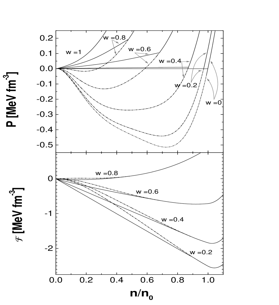
Figure 2: Pressure $P$ and free energy density $\cal{F}$ in terms of the relative density $n/n_{0}$, for ${T=2}$ MeV and several isospin asymmetries $w$. Solid lines represent the equilibrium values for stable matter, the break in the slope of these curves indicates the end point of the transition. $P$ and $\cal{F}$ evaluated for states out of equilibrium in the homogeneous one phase are shown by dashed curves.

where $n_{k}=\lambda\,n^{\prime}_{k}+(1-\lambda)\,n^{\prime\prime}_{k},\;{(k=1,2)}$, set up the conservation requirement for particle and isospin number [7].
Alternatively, the condition (5) can be stated as a set of two equations [8], Det$\mathfrak{F}\geq 0$, Tr$\mathfrak{F}\geq 0$, with $\mathfrak{F}_{ij}=\partial^{2}\mathcal{F}/\partial n_{i}\partial n_{j}$. They determine the spinodal region in the phase diagram.
In a phase transition the emerging phases satisfy the Gibbs condition for equilibrium coexistence: $\mu_{1}^{\prime}(T,n_{1}^{\prime},n_{2}^{\prime})=\mu_{1}^{\prime\prime}(T,n_{1}^{\prime\prime},n_{2}^{\prime\prime})$, $\;\mu_{2}^{\prime}(T,n_{1}^{\prime},n_{2}^{\prime})=\mu_{2}^{\prime\prime}(T,n_{1}^{\prime\prime},n_{2}^{\prime\prime})$, $\;P(T,n_{1}^{\prime},n_{2}^{\prime})=P(T,n_{1}^{\prime\prime},n_{2}^{\prime\prime})$, which fix the boundary of the binodal region. The binodal encloses the spinodal region since phase separation can occur while the condition (5) is locally satisfied [7]. For a given temperature, the coexistence conditions can be easily interpreted in terms of isobaric representations of the proton and neutron chemical potentials as functions of the proton abundance $Y=n_{1}/n$, as shown in Fig. 1. The points lying on these curves which are the vertices of a rectangle correspond to those equilibrium states which coexist in a phase separation. From these four points, the pair of neutron-proton chemical potentials on the left (right) correspond to the low (high) density coexisting phase. As it is explained below, these points are used to determine the equation of state within the binodal zone.
We have studied the equation of state of the system with variable isospin fraction at low temperatures, some results are shown in Fig. 2. We have used the Gibbs prescription and the conservation laws to evaluate the two-phase coexisting region, which produces an almost linear behavior between the end points corresponding to a single phase state. The free energy of the system is given by $\mathcal{F}(T,n_{1},n_{2})=\lambda\,\mathcal{F}(T,n^{\prime}_{1},n^{\prime}_{2})+(1-\lambda)\,\mathcal{F}(T,n^{\prime\prime}_{1},n^{\prime\prime}_{2})$, where $\lambda,n_{1}^{\prime},n_{2}^{\prime},n_{1}^{\prime\prime},n_{2}^{\prime\prime}$ had been determined previously by the Gibbs construction. It must be pointed out that for symmetric matter each phase keeps $w=0$ with a constant partial density and, as the total density increases, only the relative volume fraction changes. That is, the binodal construction reduces to the standard Maxwell procedure. In the upper panel of this figure the pressure as a function of the baryonic density is shown for several isospin asymmetries and T=2 MeV. The system becomes unstable at very low density, showing a negative compressibility. The only exception corresponds to pure neutron matter. In each case the dashed line represents the theoretical prediction without phase separation. In the lower panel the free energy for T=2 MeV is shown for a selected set of asymmetry values. As in the previous case, dashed lines correspond to the unphysical situation. It can be appreciated that the phase separation effectively causes a lowering of $\cal{F}$.

For a given temperature $T$ the pair of states satisfying the Gibbs condition determine a closed curve as the pressure ranges within the set $0\leq P\leq P_{c}(T)$. This curve is the intersection of an isothermal with the binodal surface, which extends from zero to the critical temperature $T_{c}$. We exhibit in Fig. 3 projections of the binodal into the $P-Y$ plane, corresponding to $T=2,6,$ and $10$ MeV. The area enclosed by the curve decreases with temperature, reducing to a point at $T_{c}$. In our calculations we have found $T_{c}\simeq 12.8$ MeV. The full curve can be separated into two sections with common end points, one having $Y=0.5$ and the other one with $Y=Y_{c}$, the proton abundance at the critical pressure $P_{c}(T)$. Most of the coexisting phases at a given temperature are represented by a pair of points, located in different sections. In such a case lower $Y$ values are associated with the less dense phase. This behavior is compatible with the isospin distillation observed in multifragmentation: the most dense phase approaches to isospin symmetric matter while the other one keeps the neutron excess.

For further development, we describe here the Landau parameters of the model. They are defined in terms of a second variation of the energy density [9], namely $F_{B\,B^{\prime}}=V^{2}\,\partial^{2}\mathcal{E}/\partial f_{B}\,\partial f_{B^{\prime}}$. In order to simplify the notation we have resumed in only one symbol the indices for isospin, spin and linear momentum, i. e. $B\equiv(b,s,\mathbf{p})$. The Landau’s parameters are defined as the Fourier coefficients of an expansion in terms of the Legendre polynomials

$$F^{l}_{BB^{\prime}}=(l+1/2)\int_{-1}^{1}d\nu\,P_{l}(\nu)\;V^{2}\frac{\partial^{2}\mathcal{E}(\nu)}{\partial f_{B}\,\partial f_{B^{\prime}}},$$

where $\nu=\mathbf{p}\cdot\mathbf{p}^{\prime}/(p\,p\,^{\prime})$.
Within the energy functional model used here, $\mathcal{E}$ does not depend on $\nu$, therefore the non-zero components correspond only to $l=0$, giving

$$F_{B\,B^{\prime}}^{0} = F_{b\,b^{\prime}}^{0}=\frac{2}{n}\,[F_{0}+(-1)^{b}\,G_{b\,b^{\prime}}],$$

$$F_{0}\;\; = w^{2}\,(P_{n}-P_{s})+(1+w^{2})\,x\,P_{s}^{\prime}-w^{2}\,x\,P_{n}^{\prime},$$

$$G_{b\,b^{\prime}} = (-1)^{b^{\prime}}\,(P_{n}-P_{s})+2\,\delta_{b\,b^{\prime}}\,w\,[\,P_{n}-P_{s}+x\,(P_{n}^{\prime}-P_{s}^{\prime}\,)]$$ (6)

3 Collective modes at finite temperature

Collective modes are associated to local density fluctuations that propagate in the nuclear mean field. These fluctuations are the effect of small perturbations of the occupation distribution $f_{B}$ around its equilibrium form $f_{B}^{0}$. As a conserved charge the particle density $n_{b}$ can be written as a summation over the level occupation using either $f_{B}$ or $f_{B}^{0}$,

$$n_{b}=\frac{1}{V}\sum_{s,\,\mathbf{p}}f_{B}(T)=\frac{1}{V}\sum_{s,\,\mathbf{p}}f_{B}^{0}(T)$$ (7)

The momentum can be regarded as discrete by imposing appropriate boundary conditions.

Local density fluctuations cause small deviations from the equilibrium distribution, this perturbation is assumed of periodic oscillatory nature

$$f_{B}(T,\mathbf{r},t) = f_{B}^{0}(T)+\delta f_{B}(T,\mathbf{r},t)$$ (8)

$$= f_{B}^{0}(T)+\frac{f_{B}^{\,0}(T)\,[1-f_{B}^{\,0}(T)]}{T}\,u_{B}\,e^{i\,(\mathbf{q}.\mathbf{r}-\omega\,t)}$$

Our present ansatz for the perturbation $\delta f_{B}(T,\mathbf{r},t)$ ensures that in the limit ${T\rightarrow 0}$ only the levels around the Fermi surface contribute to the zero mode propagation. The quasiparticle energies change accordingly, since in the Landau-Fermi liquid model they are obtained in a self-consistent manner from the distribution function [9, 10]

$$\delta\epsilon_{B}(T,\mathbf{r},t)=\frac{1}{V}\sum_{B^{\prime}}F_{B\,B^{\prime}}\,\delta f_{B^{\prime}}(T,\mathbf{r},t)$$ (9)

The propagation of these perturbations at low temperature is governed by the Landau’s kinetic equation. For temperatures well below the Fermi energy of the system $T\ll\epsilon_{F}$, the collision term can be neglected [11]

$$\frac{\partial f_{B}}{\partial t}+\frac{\partial f_{B}}{\partial\mathbf{r}}\,\frac{\partial\epsilon_{B}}{\partial\mathbf{p}}-\frac{\partial f_{B}}{\partial\mathbf{p}}\,\frac{\partial\epsilon_{B}}{\partial\mathbf{r}}=0$$ (10)

Introducing Eq.(8) into Eq.(10) and keeping only linear terms in the fluctuations, we obtain

$$\frac{\partial\delta f_{B}}{\partial t}+\frac{\partial\delta f_{B}}{\partial\mathbf{r}}\,\frac{\partial\epsilon_{B}}{\partial\mathbf{p}}-\frac{\partial f_{B}^{0}}{\partial\mathbf{p}}\,\frac{\partial\delta\epsilon_{B}}{\partial\mathbf{r}}=0$$ (11)

which can be further reduced to

$$\left[\omega-\frac{(\mathbf{p}\,.\mathbf{q}\,)}{m}\right]u_{B}-\frac{1}{V}\,\frac{(\mathbf{p}\,.\mathbf{q}\,)}{m}\,\sum_{B^{\prime}}F_{B\,B^{\prime}}\,\frac{f_{B^{\prime}}^{\,0}(T)\,[1-f_{B^{\prime}}^{\,0}(T)]}{T}\,u_{B^{\prime}}\,=0.$$ (12)

Since the $F_{B\,B^{\prime}}$ do not depend on $\mathbf{p}$, see Eqs. (6), we can write

$$\frac{1}{V}\,\sum_{B^{\prime}}F_{B\,B^{\prime}}\,\frac{f_{B^{\prime}}^{\,0}(T)\,[1-f_{B^{\prime}}^{\,0}(T)]}{T}\,u_{B^{\prime}}\,=\sum_{b^{\prime}}F_{b\,b^{\prime}}^{0}\,w_{b^{\prime}}$$ (13)

where

$$w_{b}=\frac{1}{\pi^{2}\,T}\,\int_{0}^{\infty}dp\,p^{2}\,f_{b}^{\,0}(T,p)\,[1-f_{b}^{\,0}(T,p)]\,u_{b}(p)$$ (14)

and we have used $u_{B}=u_{b}(p)$, $f_{B}^{\,0}(T)=f_{b}^{\,0}(T,p)$ to show explicitly their dependence on $p$. Therefore the system (12) can be rewritten in the form

$$w_{b}+\mathcal{C}_{b}(T)\,\sum_{b^{\prime}=1}^{2}\,F_{b\,b^{\prime}}^{0}\,w_{b^{\prime}}\,=0\;\;\;\;\;(b=1,2)$$ (15)

with

$$\mathcal{C}_{b}(T)=\frac{1}{\pi^{2}\,T}\,\int_{0}^{\infty}dp\,p^{2}\,f_{b}^{\,0}(T,p)\,[1-f_{b}^{\,0}(T,p)]\,\Omega_{0\,0}(V_{z}/v_{p})$$ (16)

where $v_{p}=p/m$, $V_{z}=\omega/q$ is the phase speed of the collective mode, and

$$\Omega_{0\,0}(s)=\int_{\!-1}^{+1}\frac{dy}{2}\,\frac{y}{y-s}=1+\frac{s}{2}\ln\left(\frac{s-1}{s+1}\right)$$ (17)

is the Lindhard function [9].
We shall consider the possibility of damped waves, in which case the real zero-mode frequency $\omega$ acquires an imaginary component, namely ${\omega\rightarrow\omega-i\,\eta}$. Introducing ${\delta=\eta/\omega}$, in the case of slightly damped modes where $0\leq\delta\ll 1$, we have to leading order

$$\mbox{Re}\;\mathcal{C}_{b} \!\!\!\!= \!\!\!\!\frac{1}{\pi^{2}\,T}\,\int_{0}^{\infty}\!dp\,p^{2}\;f_{b}^{\,0}(T,p)\,[1-f_{b}^{\,0}(T,p)]\,\left[\,1+\frac{V_{z}}{2\,v_{p}}\,\ln\left|\frac{V_{z}-v_{p}}{V_{z}+v_{p}}\right|\;\right]$$

$$\mbox{Im}\;\mathcal{C}_{b} \!\!\!\!= \!\!\!\!\frac{\delta}{\pi^{2}\,T}\,\int_{0}^{\infty}\!dp\,p^{2}\;f_{b}^{\,0}(T,p)\,[1-f_{b}^{\,0}(T,p)]\,\left[\,\frac{V_{z}}{2\,v_{p}}\,\ln\left|\frac{V_{z}-v_{p}}{V_{z}+v_{p}}\right|+\frac{V_{z}^{2}}{V_{z}^{2}-v_{p}^{2}}\,\right]$$ (18)

$$\!\!\!\!+ \!\!\!\!\frac{\mbox{sgn}(\delta)}{2\,\pi}\,m^{2}\,V_{z}\,f_{b}^{\,0}(T,m\,V_{z})$$

On the other hand, instability modes are characterized by $\omega=0$ and $\eta<0$, in which case

$$\mbox{Re}\;\mathcal{C}_{b} \!\!\!\!= \!\!\!\!\frac{1}{\pi^{2}\,T}\,\int_{0}^{\infty}\!dp\,p^{2}\;f_{b}^{\,0}(T,p)\,[1-f_{b}^{\,0}(T,p)]\,\left[\,1-\frac{\eta}{q\,v_{p}}\,\arctan\left(q\,v_{p}/\eta\right)\;\right]$$

$$\mbox{Im}\;\mathcal{C}_{b} \!\!\!\!= \!\!\!\!0$$ (19)

The proper frequencies are identified with the roots of the determinant of the system of equations (15), which, neglecting higher orders in $\mbox{Im}\;\mathcal{C}_{b}$, reduces to

$$[1+F_{11}^{0}\,\mbox{Re}\,\mathcal{C}_{1}][1+F_{22}^{0}\,\mbox{Re}\,\mathcal{C}_{2}]-{F_{12}^{0}}^{2}\;\mbox{Re}\,\mathcal{C}_{1}\,\mbox{Re}\,\mathcal{C}_{2} = 0$$

$$F_{11}^{0}\,[1+F_{22}^{0}\,\mbox{Re}\,\mathcal{C}_{2}]\,\mbox{Im}\,\mathcal{C}_{1}+F_{22}^{0}\,[1+F_{11}^{0}\,\mbox{Re}\,\mathcal{C}_{1}]\,\mbox{Im}\,\mathcal{C}_{2}$$

$$-{F_{12}^{0}}^{2}\;\mbox{Im}\,(\mathcal{C}_{1}\,\mathcal{C}_{2}) = 0$$ (20)

It is easy to show from Eqs.(13) and (14), that in the present model the rate of proton to neutron amplitudes is momentum independent, namely $u_{1}/u_{2}=w_{1}\mathcal{C}_{2}/w_{2}\mathcal{C}_{1}$. As done at zero temperature [10], the isospin character of the proper modes can be classified as iso-scalar (iso-vector) for ${\mbox{Re}\,(u_{1}/u_{2})>0\;(<0)}$, respectively [12].

We have verified that along the phase transition the system is composed of two stable independent phases. In particular the instability modes have completely disappeared and only stable eigenmodes are present. Furthermore, in all the cases considered here, no zero sound modes are found propagating in the lower density phase of the coexisting region. The reason is that $F_{22}^{0}$ takes always negative values in this phase.
It is convenient to define an average Fermi velocity $V_{F}$

$$V_{F}=\frac{1}{m}\,\sum_{b=1}^{2}\frac{n_{b}}{n}\,\sqrt{\frac{\int_{0}^{\infty}dp\,p^{4}\,f_{b}^{\,0}(T,p)\,[1-f_{b}^{\,0}(T,p)]}{\int_{0}^{\infty}dp\,p^{2}\,f_{b}^{\,0}(T,p)\,[1-f_{b}^{\,0}(T,p)]}}$$ (21)

as a reference to estimate deviations from the Fermi surface, which gives a measure of the validity of the approximations.
In Fig. 4 we display the typical low temperature dispersion relation for different isospin composition. At finite temperature the proper collective modes arise in pairs. One branch is slightly damped, meanwhile the other one propagates without dissipation.
For the sake of comparison, we also include the unphysical results obtained by neglecting the phase separation. This situation give rise to, among others, the instability modes. In such a case we plot ${|\eta|/q}$ instead of $V_{z}$.
For isospin symmetric matter (Fig. 4, $w=0$) the mixed phase extends up to near $n_{0}$, and as it was noticed each phase stay at constant partial density during the transition. As a consequence the collective modes propagate at constant speed $V_{z}$. At low densities there are two branches of iso-vector character, which propagate in the liquid phase and continue for higher densities, beyond the transition. In addition, a bivaluated stable iso-scalar mode appears at densities about ${1.1n_{0}}$. For iso-vector as well as for iso-scalar modes, the branch above $V_{F}$ corresponds to undamped motion. The dissipation in the iso-vector wave has an average value of ${\delta\approx 0.15}$, meanwhile the iso-scalar one has ${\delta\approx 0.09-0.19}$. Therefore, damping remains very small in agreement with our assumptions.
If phase separation in symmetric matter is disregarded (dashed lines), a double iso-vector mode appears at very low density with small values of $V_{z}$. It grows monotonously with density and joins smoothly with the solutions for the mixed stable phase. It has a moderate damping ${\delta\approx 1}$ at low densities, decreasing to ${\delta\approx 0.15}$ near $n_{0}$. At the same time, a pair of iso-scalar excitations arise at densities below ${0.8\,n_{0}}$. The lower one corresponds to a instability mode reflecting the existence of the spinodal region. In general the instability modes evolving out of thermodynamical equilibrium are iso-scalar since both isospin components are equally affected, in a process which eventually leads to clusterization [12]. The damped stable scalar mode has a dissipation coefficient growing from ${\delta\approx 1}$ to $4$ as the density is increased, mainly because it approaches the unstable configuration.
Turning to asymmetric matter (Fig. 4, $w=0.2-0.6$), this scene changes gradually as the density range of coexistence reduces with increasing $w$. At low and medium densities only iso-vector modes propagate with almost constant velocity ${V_{z}\sim 0.3}$. For ${w>0.5}$ these excitations are strongly suppressed around the medium density zone. In fact in the denser coexisting phase, the only one which can sustain collective motion, the neutron-neutron Landau parameter $F_{22}^{0}$ decreases and can take negative values when $w$ increases. For example, in the case of $w=0.6$ the parameter $F_{22}^{0}$ vanishes around ${n\approx 0.53n_{0}}$, and remains negative up to ${n\approx 0.81n_{0}}$. This explains the suppression of the density collective modes at medium densities. For supranormal densities the parameter $F_{22}^{0}$ grows again, and four collective zero modes reappear. For high isospin asymmetry these four branches are of mixed character, that is, they change from iso-vector to iso-scalar as the density increases.
It must be pointed out that in neutron rich environments such as $w=0.8$ (not shown here), two iso-vector modes with ${V_{z}\approx 0.3}$ persist in the very low density regime. This scenario of collective waves propagating in highly asymmetric nuclear matter is expected to hold within the inner crust of neutron stars. The precise structure of this crust is still doubtful, but condensed nuclear droplets immersed in a uniform fluid environment of almost pure neutron matter constitutes a plausible assumption [13, 14]. Although Coulomb effects are responsible of the existence of the droplets, the mean field properties of the asymmetrical extended fluid are governed by the nuclear forces. In fact, a liquid-gas coexistence of this low density asymmetric nuclear matter environment prevents further instabilities, as it was previously stressed. Moreover, this fluid phase can sustain coherent density fluctuations, which open a channel for neutrino dispersion. These collective excitations are similar to the spin-wave propagation investigated in [1]. Therefore it is reasonable to expect a strengthening of the effects discussed there, in particular a more pronounced reduction of the in-medium mean free path of neutrinos. A further investigation will be presented elsewhere [15].
If the phase separation is not taken into account (dashed lines), a stronger suppression of the collective modes is found, mainly because of the more pronounced decrease of $F_{22}^{0}$ with asymmetry. In this situation medium and high density excitations are affected, and already for $w=0.4$ all of them have practically been extinguished. Only the unstable and stable iso-scalar modes of sub-saturation densities survive in this case.
In general for each damped mode the parameter $\delta$ increases a bit with growing asymmetry $w$, and this enhancement is more important when only the unstable one phase is considered. We can conclude that the binodal phase transition tends to stabilize the density collective zero modes at low and medium densities.

4 Conclusions

We have applied a density functional model of the nuclear interaction fitted to describe asymmetric nuclear matter properties, to determine the coexistence regime of the liquid-gas phase transition at densities below the saturation value $n_{0}$. This study has been performed at several temperatures and isospin asymmetries. The binodal region is diminished as the temperature increases, till its critical value $T_{c}\simeq 12.8$ MeV. For a given temperature this region also decreases with growing isospin asymmetry.

We have also studied the propagation of zero sound modes at finite temperature, using a linearized collisionless Landau kinetic equation. As the method requires a stable reference state which supports density fluctuations, we have chosen the coexisting phases in the binodal instead of the unstable spinodal region. We have found that collective modes are supported only by the denser phase of the coexistence region, which favors their propagation at low total densities. Because of this, the phase speed of the collective excitations remains almost constant in a wide density range. Furthermore, since in the denser phase the proton to neutron fraction is higher than in the lighter one, it favors the stability of the density zero modes in matter with an overall neutron excess. This could have significative consequences, for example, in the scattering rates of neutrinos within the proto-neutron star matter.

Figure 1: The chemical potential $\mu$ for protons (solid lines) and neutrons (dashed lines) as a function of the proton abundance $Y$ for ${T=2}$ MeV and a set of fixed pressures $P$, ${0\leq P\leq 0.19}$ MeV/ fm³. For each isobar both curves for the proton and the neutron chemical potentials are obtained, respectively. The Gibbs construction for a given isobar is shown in the figure inset (dotted line).

Figure 3: The binodal construction as explained in the text, for several temperatures. The curves in the ${(P,Y)}$ plane enclose the zone where two independent phases coexist in thermodynamical equilibrium.

Figure 4: Zero sound dispersion $V_{z}=\omega/q$ at ${T=1}$ MeV for several asymmetries $w$ of the nuclear medium. Solid lines correspond to modes propagating either in the binodal coexisting phase with the higher density for ${n\lesssim n_{0}}$, or in the stable one phase at supra normal densities. Conversely, dashed lines represent collective propagation within the unstable homogeneous phase, as explained in the text. The label isos (isov) indicates the iso-scalar (iso-vector) character, for damped (d) and undamped (u) stable modes. Curves which change its character from iso-vector to iso-scalar are labeled mix. For the unstable iso-scalar curve the ratio ${|\eta|/q}$ is plotted. The average Fermi velocity $V_{F}$ is shown for the stable high density phase (dot line), and the unstable homogeneous phase (dash-dot-dot line).

References

- [1] N. Iwamoto and C. J. Pethick, Phys. Rev. D 25(1982)313.
- [2] V. Greco, M. Colonna, M. Di Toro, and F. Di Toro, Phys. Rev. C 67 (2003) 015203.
- [3] L. Brito, C. Providencia, A. M. Santos, S. S. Avancini, D. P. Menezes, and Ph. Chomaz, Phys. Rev. C 74 (2006) 045801.
- [4] M. Baldo, P. Schuck, and X. Viñas, Phys. Lett. B 663 (2008) 390.
- [5] P. Hohenberg and W. Kohn, Phys. Rev. 136 (1964) B864.
- [6] M. Baldo, C. Maieron, P. Schuck, and X. Viñas, Nucl. Phys. A 736 (2004) 241.
- [7] H. Muller and B. D. Serot, Phys. Rev. C 52 (1995) 2072
- [8] J. Margueron and Ph. Chomaz, Nucl. Phys. A 722 (2003) 315c.
- [9] G. Baym and C. Phethick, Landau Fermi-Liquid Theory, (John Wiley & Sons, 1991).
- [10] R. M. Aguirre and A. L. De Paoli, Phys. Rev. C 75 (2007) 045207
- [11] L. D. Landau and E. M. Lifshitz, Statistical Physics, (Pergamon Press, 1980).
- [12] V. Baran, M. Colonna, V. Greco, M. Di Toro, Phys. Rep. 410, 335 (2005).
- [13] T. Maruyama, T. Tatsumi, D. N. Voskresensky, T. Tanigawa and S. Chiba, Phys. Rev. C 72 (2005) 015802.
- [14] J. Xu, L.-W. Chen, B.-A. Li and H.-R. Ma, Astroph. J. 697 (2009) 1549.
- [15] R. M. Aguirre and A. L. De Paoli, in preparation.