Subsampling weakly dependent times series
and application to extremes

Abstract

This paper provides extensions of the work on subsampling by Bertail et al. (2004) for strongly mixing case to weakly dependent case by application of the results of Doukhan and Louhichi (1999). We investigate properties of smooth and rough subsampling estimators for distributions of converging and extreme statistics when the underlying time series is $\eta$ or $\lambda$-weakly dependent.

1 Introduction

Politis and Romano (1994) [22] established the subsampling estimator for statistics when the underlying sequence is strongly mixing. Bertail et al. (2004) [3] applied this work to subsampling estimators for distributions of diverging statistics. In particular, they constructed an approximation of the distribution of the sample maximum without any information on the tail of the stationary distribution. However the assumption on the strong mixing properties of the time series is sometimes too strong as for the class of first-order autoregressive sequences introduced and studied by Chernick (1981) [6]: for $t\in\mathbb{Z}$, let $X_{t}$ be given by

$$X_{t}=\frac{1}{r}(X_{t-1}+\varepsilon_{t}),$$ (1)

where $r\geq 2$ is an integer, $(\varepsilon_{t})_{t\in\mathbb{Z}}$ are iid and uniformly distributed on the set $\{0,1,\ldots,r-1\}$ and $X_{0}$ is uniformly distributed on $[0,1]$. Andrews (1984) [1] and Ango-Nze and Doukhan (2004) [2] (see page 1009 and Note 5 on page 1028) give arguments to derive that such models are not mixing. The results of Bertail et al. (2004) [3] can not be used although the normalized sample maximum has a non degenerate limiting distribution: let $M_{n}=\max(X_{1},\ldots,X_{n})$, then

$$\lim_{n\rightarrow\infty}\mathbb{P}\big{(}n(1-M_{n})\leq x\big{)}=1-\exp\big{(}-r^{-1}(r-1)x\big{)},\qquad\text{for all }x\geq 0\text{,}$$

(see Theorem 4.1 in Chernick (1981) [6]).

This paper is aimed at weakening the dependence conditions assumed in Bertail et al. (2004) [3] and at studying new smooth subsampling estimators adapted to our weak dependence conditions.

Doukhan and Louhichi (1999) [10] introduced a wide dependence framework that turns out in particular to apply to the previous processes and that widely improves the amount of potentially usable models. This dependence structure is addressed in Section 2. In Section 3 we introduce smooth and rough subsampling estimators for the distribution of converging statistics and studied their asymptotic properties. We consider two subsampling schemes based on overlapping and non-overlapping samples. In the next section we consider subsampling estimators for the distribution of extremes and, to fix ideas, we focus on the case of the normalized sample maximum. We first discuss sufficient conditions adapted to our weak dependence framework such that the normalized maximum converges in distribution. Then we discuss how to estimate the normalizing sequences and we derive the asymptotic properties of the subsampling estimators. A simulation study provides explicit comparisons of the various considered subsamplers in Section 5. Proofs are reported in a last section.

2 Weak dependence

Doukhan and Louhichi (1999) [10] proposed a new idea of weak dependence that makes explicit the asymptotic independence between past and future. Let us consider a strictly stationary time series $X=(X_{t})_{t\in\mathbb{Z}}$ which (for simplicity) will be assumed to be real-valued. Let us denote by $F$ its stationary distribution function. If $X$ is a sequence of iid random variables, then for all $t_{1}\neq t_{2}$, independence between $X_{t_{1}}$ and $X_{t_{2}}$ writes $\mbox{Cov}\,(f(X_{t_{1}}),g(X_{t_{2}}))=0$ for all $f,g$ with $\|f\|_{\infty},\|g\|_{\infty}\leq 1$, where $\|f\|_{\infty}$ denotes the surpremum norm of $f$. For a sequence of dependent random variables, we would like that $\mbox{Cov}\,(f($‘$past$’$),g($‘$future$’$))$ is small when the distance between the past and the future is sufficiently large.
More precisely, for $h:\mathbb{R}^{u}\rightarrow\mathbb{R}$ ($u\in\mathbb{N}^{\ast}$) we define

$\displaystyle{\mathrm{Lip}\,}h=\sup_{(y_{1},\ldots,y_{u})\neq(x_{1},\ldots,x_{u})\in\mathbb{R}^{u}}\frac{\left|h(y_{1},\ldots,y_{u})-h(x_{1},\ldots,x_{u})\right|}{\|y_{1}-x_{1}\|+\cdots+\|y_{u}-x_{u}\|}.$

Definition 1

[10] The process $X$ is $(\varepsilon,\Psi)$-weakly dependent process if, for some classes of functions $\mathcal{F}_{u},\mathcal{G}_{v}$, $E^{u},E^{v}\rightarrow\mathbb{R},u,v\geq 1$:

$$\varepsilon(r)=\sup\frac{\left|{{\mbox{Cov}\,}}\Big{(}f(X_{s_{1}},\ldots,X_{s_{u}}),g(X_{t_{1}},\ldots,X_{t_{v}})\Big{)}\right|}{\Psi(f,g)}\rightarrow_{r\rightarrow\infty}0$$

where the $\sup$ bound is relative to $u,v\geq 1$, $s_{1}\leq\cdots\leq s_{u}\leq t_{1}\leq\cdots\leq t_{v}$ with $r=t_{1}-s_{u}$, and $f,g$ satisfy $\mbox{Lip}\,f,\mbox{Lip}\,g<\infty$ and $\|f\|_{\infty}\leq 1$, $\|g\|_{\infty}\leq 1$.

The following distinct functions $\Psi$ yield $\eta$, and $\lambda$ weak dependence coefficients:

$\begin{array}[]{lllcr}\text{if }\Psi(f,g)&=&u\mbox{Lip}\,f+v\mbox{Lip}\,g,&\mbox{then}&\epsilon(r)=\eta(r),\\ &=&u\mbox{Lip}\,f+v\mbox{Lip}\,g+uv\mbox{Lip}\,f\cdot\mbox{Lip}\,g,&\mbox{then}&\epsilon(r)=\lambda(r),\end{array}$

Note that $\lambda$-weak dependence includes $\eta$-weak dependence. A main feature of Definition 1 is to incorporate a much wider range of classes of models than those that might be described through a mixing condition (i.e. $\alpha$-mixing, $\beta$-mixing, $\rho$-mixing, $\phi$-mixing, …, see Doukhan (1994) [9])) or association condition (see Chapters 1-3 in Dedecker et al. (2007) [8]). Limit theorems and very sharp results have been proved for this class of processes (see Chapters 6-12 in Dedecker et al. (2007) [8] for more information).

We now provide a non-exhaustive list of weakly dependent sequences with their weak dependence properties. This will prove how wide is the range of potential applications.

Example 1

• The Bernoulli shift with independent inputs $(\xi_{t})_{t\in\mathbb{Z}}$ is defined as $X_{t}=H((\xi_{t-j})_{j\in\mathbb{Z}}),$ $H:\mathbb{R}^{\mathbb{Z}}\rightarrow\mathbb{R},$ $(\xi_{i})_{i\in\mathbb{Z}}$ iid. The process $(X_{t})_{t\in\mathbb{Z}}$ is $\eta$-weakly dependent with $\eta(r)=2\delta_{[r/2]}^{m\wedge 1}$ if

  $$\mathbb{E}\big{|}H\big{(}\xi_{j},j\in\mathbb{Z}\big{)}-H\big{(}\xi_{j}\mbox{I1}_{|j|<r},j\in\mathbb{Z}\big{)}\big{|}\leq\delta_{r}\downarrow 0\quad(r\uparrow\infty).$$

  Two particular (causal) examples are given by:

  - The first-order autoregressive sequences with discrete innovations given by (1). This process is not strongly mixing but it is $\eta$-weakly dependent process such that $\eta(k)=O\left(r^{-k}\right)$.

  - The LARCH model with Rademacher iid inputs:

  $$X_{t}=\xi_{t}(1+aX_{t-1}),\qquad\mathbb{P}(\xi_{0}=\pm 1)=\frac{1}{2}.$$ (2)

  If $a<1$, there exists a unique stationary solution (see Dedecker et al. (2007) [8]). Doukhan, Mayo and Truquet (2008) [12] proved that if $a\in\left((3-\sqrt{5})/2,1/2\right]$ the stationary solution $X_{t}=\xi_{t}+\sum_{j\geq 1}a^{j}\xi_{t}\cdots\xi_{t-j}$ is not strongly mixing, but $X$ is a $\eta$-weakly dependent process such that $\eta(k)=O\left(a^{k}\right)$.

• If $X$ is either a Gaussian or an associated process, then $X$ is $\lambda$-weakly dependent and

  $$\lambda(r)=O\left(\sup_{i\geq r}|\mbox{Cov}\,(X_{0},X_{i})|\right)$$

  (see Doukhan and Louhichi (1999) [10]).

• If $X$ is a $GARCH(p,q)$ process or, more generally, a $ARCH(\infty)$ process such that $X_{k}=\rho_{k}\xi_{k}$ with $\rho_{k}^{2}=b_{0}+\sum_{j=1}^{\infty}b_{j}X_{k-j}^{2}$ for $k\in\mathbb{Z}$ and if,

  - it exists $C>0$ and $\mu\in]0,1[$ such that $\forall j\in\mathbb{N}$, $0\leq b_{j}\leq C\mu^{j}$, then $X$ is $\lambda$-weakly dependent process with $\lambda(r)=O\left(e^{-c\sqrt{r}}\right)$ and $c>0$ (this is the case of $GARCH(p,q)$ processes).

  - it exists $C>0$ and $\nu>1$ such that $\forall j\in\mathbb{N}$, $0\leq b_{j}\leq Cj^{-\nu}$, then $X$ is $\lambda$-weakly dependent process with $\lambda(r)=O\left(e^{-r}\right)$.

3 Subsampling the distribution of converging statistics

Politis and Romano (1994) [22] introduced the methodology of “subsampling” to give consistent approximations of confidence intervals for some parameters of the distribution of the observations. They established the validity of their methodology for general strongly mixing sequences under the assumption that the considered statistics converge with a known rate.

We consider here a sequence of statistics $S_{n}=s_{n}(X_{1},\ldots,X_{n})$ for $n=1,2,\ldots$ Let $\mathbb{K}_{n}$ be the cumulative distribution function of $S_{n}$, $\mathbb{K}_{n}(x)=P(S_{n}\leq x)$. We assume that $S_{n}$ is a sequence of converging statistics in the sense that $\mathbb{K}_{n}$ has a limit which is denoted by $\mathbb{K}$. We assume that the statistics satisfy one of the two following assumptions:

- Convergent statistics:

$$r_{n} = \sup_{x\in\mathbb{R}}\Big{|}\mathbb{K}_{n}(x)-\mathbb{K}(x)\Big{|}\rightarrow_{n\rightarrow\infty}0,\qquad\|\mathbb{K}^{\prime}\|_{\infty}<\infty.$$

where $$\mathbb{K}^{\prime}$$ denotes the density of this limit distribution.

- Concentration condition:

$$\sup_{x\in\mathbb{R}} \mathbb{P}(S_{n}\in[x,x+z])\leq C(n)z^{c}\qquad(\forall z>0)$$

for suitable constants $$c,C(n)>0 n=1,2,\ldots$$, if

We also consider a bandwidth function $b\equiv b_{n}\rightarrow\infty$ such that $\lim_{n\rightarrow\infty}n/b=\infty$ and two subsampling schemes

$$Y_{b,i} = (X_{i+1},\ldots,X_{i+b}),\qquad N=n-b,\qquad\mbox{ overlapping samples},$$ (5)

$$Y_{b,i} = (X_{(i-1)b+1},\ldots,X_{ib}),\qquad N=\frac{n}{b},\qquad\mbox{ non-overlapping samples}.$$ (6)

Then we introduce a smooth and a rough subsampling estimator for $\mathbb{K}$

$$\widetilde{\mathbb{K}}_{b,n}(x)=\,\frac{1}{N}\sum_{i=0}^{N-1}\varphi\left(\frac{s_{b}(Y_{b,i})-x}{\epsilon_{n}}\right),$$ smooth subsampled statistics, (7)

$$\widehat{\mathbb{K}}_{b,n}(x)=\,\frac{1}{N}\sum_{i=0}^{N-1}\mbox{I1}\,(s_{b}(Y_{b,i})\leq x),$$ rough subsampled statistics, (8)

where I1 is the indicator function. Here, ${\epsilon_{n}}\downarrow 0$ and $\varphi$ is the non-increasing continuous function such that $\varphi=1$ or 0 according to $x\leq 0$ or $x\geq 1$ and which is affine between $0$ and $1$. From the convergent statistics assumption (3), one easily checks that the bias of our first estimator is bounded the following way:

$$\sup_{x\in\mathbb{R}}\Big{|}\mathbb{E}[\widetilde{\mathbb{K}}_{b,n}(x)]-\mathbb{K}(x)\Big{|}\leq r_{b}+\epsilon_{n}\|\mathbb{K}^{\prime}\|_{\infty}.$$ (9)

Remark 1 (discussing assumptions)

• The rough subsampler (8) is the usual one. However in order to derive uniform a.s. convergence this estimator will need the stronger concentration condition (3), due to the specific problems related to weak dependence. Indeed this estimate is based on indicators which are not Lipschitz functions and bounds for covariances are more hard to handle. Besides the simple stationary Markov case for which existence of a bounded transition probability density is enough to assert that $c=1$, examples for which those concentration conditions are proved may be found in Doukhan and Wintenberger (2007, 2008) [13] and [14].

• The two techniques of subsampling developed here are based on overlapping or non-overlapping samples; it is clear that (5) is much more economic in terms of the sample size $n$ since the corresponding sum runs over $(n-b)$ indices while this number is only $n/b$ in case (6). However the latter condition assumes less restrictive weak dependence, since the involved $b-$samples are more distant.

In order to prove either uniform strong or weak laws of large numbers, we aim at bounding the $p-$th centered moments of $\widetilde{\mathbb{K}}_{b,n}(x)$ and $\widehat{\mathbb{K}}_{b,n}(x)$ defined as

$$\widetilde{\Delta}_{b,n}^{(p)}(x)=\left|\mathbb{E}\left[\widetilde{\mathbb{K}}_{b,n}(x)-\mathbb{E[}\widetilde{\mathbb{K}}_{b,n}(x)]\right]^{p}\right|,\qquad\widehat{\Delta}_{b,n}^{(p)}(x)=\left|\mathbb{E}\left[\widehat{\mathbb{K}}_{b,n}(x)-\mathbb{E[}\widehat{\mathbb{K}}_{b,n}(x)]\right]^{p}\right|.$$

Borel-Cantelli lemma will then allow to conclude.

For simplicity we set the notation $L(b)={\mathrm{Lip}\,}s_{b}.$ Moreover, for two sequences $a\equiv(a_{n})$ and $b\equiv(b_{n})$, $a\prec b$ means that there exists a positive constant $c$ such that, for all $n$, $a_{n}\leq bc_{n}$.

We first give results for the smooth subsampler by considering the convergence condition (3). Almost sure convergence is obtained to the price of restrictive conditions that meets all the qualities required in our framework.

Theorem 1 (Smooth subsampler)

Assume the convergence assumption (3) hold. Let $\delta>0$ and $p\in\mathbb{N}^{\ast}$. Assume moreover that if respectively the overlapping setting is used and one among the following relations hold as $n\rightarrow\infty$

$$\underline{\eta\mbox{-dependence:}} \sum_{t=0}^{\infty}(t+1)^{p-2}\eta(t)<\infty,\qquad\frac{b}{n}\left(1\vee\frac{L(b)}{\epsilon_{n}}\right)\prec n^{-\delta},\mbox{ or}$$

$$\underline{\lambda\mbox{-dependence:}} \sum_{t=0}^{\infty}(t+1)^{p-2}\lambda(t)<\infty,\qquad\frac{b}{n}\left(1\vee\frac{L(b)}{\epsilon_{n}}\vee\frac{bL(b)^{2}}{\epsilon_{n}^{2}}\right)\prec n^{-\delta},$$

or the non-overlapping setting is used and

$$\underline{\eta\mbox{-dependence:}} \sum_{t=0}^{n-1}(t+1)^{p-2}\eta(t)\prec b^{p-2},\qquad\frac{b}{n}\left(1\vee\frac{bL(b)}{\epsilon_{n}}\right)\prec n^{-\delta},\mbox{ or}$$

$$\underline{\lambda\mbox{-dependence:}} \sum_{t=0}^{n-1}(t+1)^{p-2}\lambda(t)\prec b^{p-2},\quad\frac{b}{n}\left(1\vee\frac{bL(b)}{\epsilon_{n}}\vee\frac{bL(b)^{2}}{\epsilon_{n}^{2}}\right)\prec n^{-\delta}.$$

Then

$$\widetilde{\Delta}_{b,n}^{(p)}(x)\prec n^{-[\frac{p}{2}]\delta}.$$

Hence, from Borel-Cantelli Lemma, if $p/2\in\mathbb{N}$ is such that $p\delta>2$, then

$$\sup_{x\in\mathbb{R}}\left|\widetilde{\mathbb{K}}_{b,n}(x)-\mathbb{K}(x)\right|\rightarrow_{n\rightarrow\infty}0\qquad\mbox{a.s.}$$

Finally, for completeness, we give results for the rough subsampler by considering successively the convergence condition (3) and the concentration condition (3).

Theorem 2 (Rough subsampler under condition (3))

Assume that the convergence assumption (3) holds. If respectively the overlapping setting is used and one among the following relations hold

$$\underline{\eta\mbox{-dependence:}} \displaystyle\sum_{t=0}^{\infty}\eta(t)^{\frac{1}{2}}<\infty, \lim_{n\rightarrow\infty}\frac{b}{n}\left(1\vee\frac{L({b})}{\sqrt{{b}}}\right)=0$$

$$\underline{\lambda\mbox{-dependence:}} \displaystyle\sum_{t=0}^{\infty}\lambda(t)^{\frac{2}{3}}<\infty, \lim_{n\rightarrow\infty}\frac{b}{n}\left(1\vee\left(\frac{L(b)^{4}}{{b}}\right)^{\frac{1}{3}}\vee\left(\frac{L({b})}{{b}}\right)^{\frac{2}{3}}\right)=0$$

or the non-overlapping setting is used and

$$\underline{\eta\mbox{-dependence:}} \displaystyle\sum_{t=0}^{\infty}\eta(t)^{\frac{1}{2}}<\infty, \lim_{n\rightarrow\infty}\frac{{b}}{n}\left(1\vee\sqrt{{b}}L({b})\right)=0$$

$$\underline{\lambda\mbox{-dependence:}} \displaystyle\sum_{t=0}^{\infty}\lambda(t)^{\frac{2}{3}}<\infty, \lim_{n\rightarrow\infty}\frac{{b}}{n}\left(1\vee(bL({b})^{2})^{\frac{2}{3}}\vee\left({b}L({b})^{2}\right)^{\frac{1}{3}}\right)=0,$$

then $\lim_{n\rightarrow\infty}\widehat{\Delta}_{b,n}^{(2)}(x)=0$ and

$$\lim_{n\rightarrow\infty}\sup_{x\in\mathbb{R}}\left|\widehat{\mathbb{K}}_{b,n}(x)-\mathbb{K}(x)\right|=0,\quad\mbox{in probability.}$$

Theorem 3 (Rough subsampler under condition (3))

Assume that the concentration assumption (3) holds. Let $\delta>0$ and $p\in\mathbb{N}^{\ast}$. Assume moreover that if respectively the overlapping setting is used and one among the following relations hold, as $n\rightarrow\infty$,

$\eta$-dependence:  $\displaystyle\sum_{t=0}^{\infty}(t+1)^{p-2}\eta(t)^{\frac{2+c}{1+c}}<\infty,$

$$\frac{b}{n}\left(1\vee\left(C(b)b^{-1}L(b)^{c}\right)^{\frac{1}{1+c}}\vee\left(bL(b)^{2+c}\right)^{\frac{1}{1+c}}\right)\prec n^{-\delta},$$

$\lambda$-dependence:  $\displaystyle\sum_{t=0}^{\infty}(t+1)^{p-2}\lambda(t)^{\frac{1+c}{2+c}}<\infty$,

$$\frac{b}{n}\left(1\vee(C(b)^{2}b^{c-2}L(b)^{2c})^{\frac{1}{2+c}}\vee(C(b)b^{-2}L(b)^{c})^{\frac{1}{2+c}}\vee(C(b)b^{c-2}L(b)^{2c})^{\frac{1}{2+c}}\right)\prec n^{-\delta}$$

or the non-overlapping setting is used

$\eta$-dependence:   $\displaystyle\sum_{t=0}^{n-1}(t+1)^{p-2}\eta(t)^{\frac{2+c}{1+c}}\prec b^{p-2},$

$$\frac{b}{n}\left(1\vee\left(C(b)(bL(b))^{c}\right)^{\frac{1}{1+c}}\vee(bL(b))^{\frac{2+c}{1+c}}\right)\prec n^{-\delta},$$

$\lambda$-dependence:  $\displaystyle\sum_{t=0}^{n-1}(t+1)^{p-2}\lambda(t)^{\frac{1+c}{2+c}}\prec b^{p-2}$

$$\frac{b}{n}\Big{(}1\vee(C(b)(bL(b))^{c})^{\frac{2}{2+c}}\vee(C(b)(bL(b))^{c})^{\frac{1}{2+c}}\vee(C(b)(bL(b))^{2c})^{\frac{1}{2+c}}\Big{)}\prec n^{-\delta}.$$

Then

$$\widehat{\Delta}_{b,n}^{(p)}(x)\prec n^{-[\frac{p}{2}]\delta}.$$

Hence, if $p/2\in\mathbb{N}$ is such that $p\delta>2$, then

$$\sup_{x\in\mathbb{R}}\left|\widehat{\mathbb{K}}_{b,n}(x)-\mathbb{K}(x)\right|\rightarrow_{n\rightarrow\infty}0\qquad\mbox{a.s.}$$

The rough subsampler needs a very strong concentration assumption and excessively intricate weak dependence conditions for uniform strong consistency. Such conditions are definitely hard to derive in the most general settings.

Remark 2

• For Theorem 1 and 3, if one of the above mentioned relations hold with $p=2$, then we obtain the same result but only with respect to the convergence in probability.

• Choosing the procedure. The overlapping frame yields a more expensive procedure, in terms of the assumptions of the bandwidth. A strange feature of the results is that, for the a.s. convergence case where moments with high order need to be calculated, that weak dependence assumptions are weaker in this case.

• Monitoring the smoothing parameter $\epsilon_{n}$. A bit more may be found from the previous result. The square of bias of our statistics is indeed given as $O(\epsilon_{n}^{2}+r_{b}^{2})$ while now the order of variance is respectively

  Overlapping $$\eta\mbox{-dependence:} \frac{b}{n}\left(1\vee\frac{L(b)}{\epsilon_{n}}\right),$$

  $$\lambda\mbox{-dependence:} \frac{b}{n}\left(1\vee\frac{L(b)}{\epsilon_{n}}\vee\frac{bL(b)^{2}}{\epsilon_{n}^{2}}\right),$$

  Non-overlapping $$\eta\mbox{-dependence:} \frac{b}{n}\left(1\vee\frac{bL(b)}{\epsilon_{n}}\right),$$

  $$\lambda\mbox{-dependence:} \frac{b}{n}\left(1\vee\frac{bL(b)}{\epsilon_{n}}\vee\frac{bL(b)^{2}}{\epsilon_{n}^{2}}\right).$$

  Hence eg. under $\eta-$dependence a reasonable choice for this parameter is $\epsilon_{n}$$=(bL(b)/n)^{1/3}$ (resp. $(b^{2}L(b)/n)^{1/3}$ for the non-overlapping case). Notice however that the order of the quadratic approximation of our subsampler is always bounded by $\max\{r_{b}^{2},b/n\}$.
  If the process is centered, the CLT writes with the statistics $t_{b}(x_{1},\ldots,x_{b})=(x_{1}+\cdots+x_{b})/\sqrt{b}$; here $L(b)=b^{-1/2}$ and we choose respectively $\epsilon_{n}$$=b^{1/6}n^{-1/3}$, or $b^{1/2}n^{-1/3}$.

• Uniformity. The fact that $\varphi$ is monotonous is essential in order to derive uniform convergence of those subsamplers; it indeed allows to use the standard variant of Dini Theorem.

• Confidence bands. For a statistical validation of the technique, a CLT theorem is also required. A first step for such a central limit theorem is to precise the asymptotic variance. For simplicity we shall mention hard subsampling of a convergent sequence of statistics (3). In this case $\lim_{b}\mathbb{K}_{b}(x)=\mathbb{K}(x)$ and the variance of $\widehat{\mathbb{K}}_{b,n}$ should involve also $t_{b,i}(x)=\mbox{Cov}\,(\mbox{I1}_{s_{b}(Y_{n,0})\leq x},\mbox{I1}_{s_{b}(Y_{n,i})\leq x})$. As in the proofs a concentration assumption leads to $|t_{b,j}(x)|\leq\mbox{const}\cdot\eta^{c}(j-b)$ (resp. $\leq\mbox{const}\cdot\lambda^{c}(j-b)$) in the case $j>b$ and for a suitable constant $0<c<1$; for the non-overlapping scheme we only need $j\geq 1$ and $j-b$ is now replaced by $(j-1)b$. The claim is now that

  $$n\mbox{Var}\,\widehat{\mathbb{K}}_{b,n}(x)\rightarrow\sum_{k}t_{|k|}(x),\quad t_{0}(x)=\mathbb{K}(x)(1-\mathbb{K}(x)),\ t_{j}(x)=\lim_{b\rightarrow\infty}t_{b,j}(x).$$

  An analogue result in the nonverlapping case writes more simply

  $$\frac{n}{b}\mbox{Var}\,\widehat{\mathbb{K}}_{b,n}(x)\rightarrow t_{0}(x)+2t_{1}(x),\ t_{0}(x)=\mathbb{K}(x)(1-\mathbb{K}(x)),\ t_{1}(x)=\lim_{b\rightarrow\infty}t_{b,1}(x).$$

  This is a first step for a CLT because in both cases the normalization coefficient is $N$. Anyway proving a CLT involves a more precise analysis of the situation and the use of Lindeberg method with Bernstein blocs. However, the knowledge of this limit variance already provides a reasonable confidence band for this estimator.

4 Subsampling the distribution of extremes

Bertail et al. (2004) [3] studied subsampling estimators for distributions of diverging statistics, but imposed that the underlying sequence is strongly mixing. We aim at generalizing their results for weakly dependent sequences. Instead of considering the general case, we focus on the sample maximum because we are able to give sufficient conditions such that the normalized sample maximum converges in distribution under the weak dependence assumption. Note however that the results can easily be generalized provided that it is possible to compute the Lipschitz coefficient of the function used to define the diverging statistics.

4.1 Convergence of the sample maximum

We first discuss conditions for convergence in distribution of the normalized sample maximum of the weakly dependent sequence.

Let $x_{F}=\sup\{x:F(x)<1\}$ be the upper end point of $F$ and $\bar{F}:=1-F$. We say that the stationary distribution $F$ is in the domain attraction of the generalized extreme value distribution with index $\gamma$, $-\infty<\gamma<\infty$, if there exists a positive and measurable function $g$ such that for $1+\gamma x>0$

$$\lim_{u\rightarrow x_{F}}\bar{F}(u+xg(u))/\bar{F}(u)=(1+\gamma x)^{-1/\gamma}\text{.}$$

Then there exist sequences $(u_{n})_{n\geq 1}$ and $(v_{n})_{n\geq 1}$ such that $u_{n}>0$ and

$$\lim_{n\rightarrow\infty}F^{n}(w_{n}(x))=G_{\gamma}(x):=\left\{\begin{tabular}[]{ll}$\exp(-(1+\gamma x)_{+}^{-1/\gamma})$&if $\gamma\neq 0,$\\ $\exp(-\exp(-x))$&if $\gamma=0,$\end{tabular}\right.$$ (10)

where $w_{n}(x)=x/u_{n}+v_{n}$. Let $q\left(t\right)=F^{\leftarrow}\left(1-t^{-1}\right)$ where $F^{\leftarrow}$ is the generalised inverse of $F$. Then $(u_{n})_{n\geq 1}$ and $(v_{n})_{n\geq 1}$ can be chosen as

$$v_{n} = q\left(n\right)$$

$$u_{n}^{-1} = \left\{\begin{tabular}[]{ll}$(-\gamma)(x_{F}-q\left(n\right))$&if $\gamma<0,$\\ $q\left(ne\right)-q\left(n\right)$&if $\gamma=0,$\\ $\gamma q\left(n\right)$&if $\gamma>0.$\end{tabular}\right.$$

Let us introduce the extremal dependence coefficient

$$\beta_{n,l}=\sup|\mathbb{P}\left(X_{i}\leq w_{n}(x),i\in A\cup B\right)-\mathbb{P}\left(X_{i}\leq w_{n}(x),i\in A\right)\mathbb{P}\left(X_{i}\leq w_{n}(x),i\in B\right)|\text{,}$$

where the sets $A$ and $B$ are such that : $A\subset\left\{1,\ldots,k\right\}$, $B\subset\left\{k+l,\ldots,n\right\}$, and $1\leq k\leq n-l$.

O’Brien (1987) [19] gave sufficient conditions such that the normalized sample maximum $u_{n}(M_{n}-v_{n})$ converges in distribution when the stationary distribution is in the domain attraction of some extreme value distributions.

Theorem 4

[19] Assume that $F$ is in the domain attraction of the extreme value distribution with index $\gamma$. Let $\left(a_{n}\right)$ be a sequence of positive integers such that $a_{n}=o\left(n\right)$ as $n\rightarrow\infty$ and

$$\lim_{n\rightarrow\infty}\frac{\mathbb{P}(M_{a_{n}}>w_{n}(x))}{a_{n}\bar{F}(w_{n}(x))}=\theta\in(0,1].$$ (12)

Assume that there exists a sequence $\left(l_{n}\right)$ of positive integers such that

$$l_{n}=o\left(a_{n}\right)\text{\qquad and\qquad}\frac{n}{a_{n}}\beta_{n,l_{n}}\rightarrow_{n\rightarrow\infty}0\text{\qquad as }n\rightarrow\infty.$$ (13)

Then

$$\lim_{n\rightarrow\infty}\mathbb{P}(M_{n}\leq w_{n}(x))=\left\{\begin{tabular}[]{ll}$\exp(-\theta(1+\gamma x)_{+}^{-1/\gamma})$&if $\gamma\neq 0,$\\ $\exp(-\theta\exp(-x))$&if $\gamma=0.$\end{tabular}\right.$$ (14)

The constant $\theta$ is referred to as the extremal index of $X$ (see Leadbetter et al. (1983) [18]). Note that any $l_{n}=o\left(n\right)$ such that $\beta_{n,l_{n}}\rightarrow 0$ as $n\rightarrow\infty$ can be used in constructing a sequence $a_{n}$ such that (13) is satisfied by taking $a_{n}$ equal to the integer part of $\max(n\beta_{n,l_{n}}^{1/2},(nl_{n})^{1/2})$. The condition $\beta_{n,l_{n}}\rightarrow 0$ as $n\rightarrow\infty$ is known as the $D(w_{n})$ condition (see Leadbetter (1974) [16]).

We provide an equivalent theorem when $X$ is assumed to be either $\eta$ or $\lambda$-weakly dependent.

Theorem 5

Assume that $F$ is an absolutely continuous distribution in the domain of attraction of the extreme value distribution with index $\gamma$ such that for $1+\gamma x>0$

$$\lim_{n\rightarrow\infty}\frac{\partial}{\partial x}F^{n}(w_{n}(x))=\frac{\partial}{\partial x}G_{\gamma}(x).$$ (15)

Let $\left(a_{n}\right)$ be a sequence of positive integers such that $a_{n}=o\left(n\right)$ as $n\rightarrow\infty$ and (12) holds. Assume that there exists a sequence $\left(l_{n}\right)$ of positive integers such that $l_{n}=o\left(a_{n}\right)$ ($n\rightarrow\infty$). If $X$ is $\eta$-weakly dependent and

$$\frac{n}{a_{n}}\left(n\eta(l_{n})u_{n}\right)^{1/2}\rightarrow_{n\rightarrow\infty}0,$$

or if $X$ is $\lambda$-weakly dependent and

$$\frac{n}{a_{n}}\left(\left[n\lambda(l_{n})u_{n}\right]^{1/2}\vee\left[na_{n}\lambda(l_{n})u_{n}^{2}\right]^{1/3}\right)\rightarrow_{n\rightarrow\infty}0,$$

then (14) holds.

4.2 Subsampling the distribution of the normalized sample maximum

Consider the sequence of extreme statistics

$$M_{n}=m_{n}(X_{1},\ldots,X_{n})=\max_{1\leq i\leq n}X_{i}.$$

Set $\mathbb{H}_{n}(x)=\mathbb{P}(M_{n}\leq x)$. Restate the smooth subsampling estimates for non-normalized extremes by

$$\widetilde{\mathbb{H}}_{b,n}(x)=\frac{1}{N}\sum_{i=0}^{N-1}\varphi\left(\frac{m_{b}(Y_{b,i})-x}{\epsilon_{n}}\right).$$ (16)

Assume, under the assumption of Theorem 5, that (3) adapted to normalized extremes holds, i.e.

$$r_{n}=\sup_{x\in\mathbb{R}}|\mathbb{H}_{n}(w_{n}(x))-\mathbb{H}(x)|\rightarrow_{n\rightarrow\infty}0.$$

where $\mathbb{H=}G_{\gamma}^{\theta}$.

Following the lines of Bertail et al. (2004) [3], we have to impose conditions on the median and the distance between two quantiles of the limiting distribution in order to be able to identify it. The median of the limiting distribution to estimate is assumed to be equal to $0$ and the distance between the quantiles is assumed to be equal to $1$. Fix $0<t_{1}<t_{2}<1$. Then the normalizing sequences can be estimated by

$$\widetilde{v}_{b,n}=\widetilde{\mathbb{H}}_{b,n}^{\leftarrow}\left(\frac{1}{2}\right),\qquad\widetilde{u}_{b,n}=\left|\widetilde{\mathbb{H}}_{b,n}^{\leftarrow}(t_{2})-\widetilde{\mathbb{H}}_{b,n}^{\leftarrow}(t_{1})\right|^{-1}.$$ (17)

Let $C=\mathbb{H}^{\leftarrow}(t_{2})-\mathbb{H}^{\leftarrow}(t_{1})$. Using that here $L(b)={\mathrm{Lip}\,}m_{b}=1$, we derive from Theorem 1 and Theorem 4 in Bertail et al. (2004) [3] the following theorem.

Theorem 6

Assume that the conditions of Theorem 5 hold. Let $\delta>0$ and $p\in\mathbb{N}^{\ast}$.

The relation $\left|\mathbb{E}\left[\widetilde{\mathbb{H}}_{b,n}(w_{b}(x))-\mathbb{E[}\widetilde{\mathbb{H}}_{b,n}(w_{b}(x))]\right]^{p}\right|\prec n^{-[\frac{p}{2}]\delta}$ holds if we assume that $\lim_{n\rightarrow\infty}\epsilon_{n}u_{b}=0$ and respectively (as $n\rightarrow\infty$) that:

• in the overlapping case,
  $\eta$-weak dependence,  $\displaystyle\sum_{t=0}^{\infty}(t+1)^{p-2}\eta(t)<\infty,\quad\frac{b}{n^{1-\delta}\epsilon_{n}}\prec 1,$ or
  $\lambda$-weak dependence,  $\displaystyle\sum_{t=0}^{\infty}(t+1)^{p-2}\lambda(t)<\infty,\quad\frac{b}{n^{1-\delta}\epsilon_{n}^{2}}\prec 1,$

• in the non-overlapping case,
  $\eta$-weak dependence,  $\displaystyle\sum_{t=0}^{n-1}(t+1)^{p-2}\eta(t)\prec b^{p-2},\quad\frac{b^{2}}{n^{1-\delta}\epsilon_{n}}\prec 1,$ or
  $\lambda$-weak dependence,  $\displaystyle\sum_{t=0}^{n-1}(t+1)^{p-2}\lambda(t)\prec b^{p-2},\quad\frac{b^{2}}{n^{1-\delta}\epsilon_{n}^{2}}\prec 1.$

Hence, if $p/2\in\mathbb{N}$ is such that $p\delta>2$, then

$$\sup_{x\in\mathbb{R}}\left|\widetilde{\mathbb{H}}_{b,n}\left(\widetilde{v}_{b,n}+\frac{x}{\widetilde{u}_{b,n}}\right)-\mathbb{H}\left(\mathbb{H}^{\leftarrow}\left(\frac{1}{2}\right)+Cx\right)\right|\rightarrow_{n\rightarrow\infty}0\qquad\mbox{a.s.}$$

5 Simulation study

The finite sample properties of our subsampling estimators are now compared in a simulation study. We consider both rough and smooth subsampling estimators when they are computed with the overlapping or non overlapping schemes.

Sequences of length $n=2$,$000$ and $n=5,000$ have been simulated from the first-order autoregressive process of Example (1)

$$X_{t}=\frac{1}{r}(X_{t-1}+\varepsilon_{t}),$$

where $(\varepsilon_{t})_{t\in\mathbb{Z}}$ are iid and uniformly distributed on the set $\{0,1,\ldots,r-1\}$ and $r$ is equal to $3$. It is well-known that the asymptotic condition (14) holds with $\gamma=-1$, $\theta=r^{-1}(r-1)$, $u_{n}=n$ and $v_{n}=1-n^{-1}$. Following the approach presented in the previous Subsection 4.2, we have to fix conditions on the median and two quantiles of the limiting distribution. We choose $t_{1}=1/4$ and $t_{2}=3/4$. The limiting distribution becomes

$$\mathbb{K}(x)=e^{-\theta(1-(x-d)/c)},\qquad x\leq c+d,$$

where $c=\theta/\ln 3$ and $d=(\ln 2-\theta)/\ln 3$. The normalization coefficients $\bar{u}_{n}$ and $\bar{v}_{n}$ such that

$$\lim_{n\rightarrow\infty}\mathbb{P}(\bar{u}_{n}(M_{n}-\bar{v}_{n})\leq x)=\mathbb{K}(x)$$

are given by

$$\bar{v}_{n}=v_{n}-c^{-1}u_{n}^{-1}d,\qquad\bar{u}_{n}=cu_{n}.$$ (18)

We first simulate a sequence of length $n=2,000$ and plot the estimators of the limiting distribution in Figure 1. As expected, smoothing estimators yield smoother curves. The differences between the estimators are small but the smoothed versions need less strong assumptions for their trajectorial convergence.

Figure 1: AR(1) process - The rough (dashed) and smooth (solid) subsampling estimators computed with the non-overlapping scheme (thin) and with the overlapping scheme (thick) for a sequence of length $n=2,000$. $b=50$, $\epsilon=0.05$.

Monte Carlo approximations to the quantiles and the means of the estimators have been then computed from $1,000$ simulated sequences.

The properties of our rough and smooth subsampling estimators computed with the non-overlapping scheme are shown in the two upper graphs in Figure 2. There are very few differences between both estimators according to their quantiles and their means. Their biases are negligible for all the value of $x$. The confidence intervals with level $90\%$ (gray zone) vanish when $x$ goes to $0$ because $0$ is the median of the empirical distribution, but also the median of the asymptotic distribution. We may compare the quantiles and the means of our estimators with those obtained when the normalization coefficients given by (17) are replaced by the theoretical normalization coefficients given by (18) (see the two lower graphs in Figure 2). First note that the bias become negative when $x$ is smaller than the median. Second the confidence intervals are obviously not equal to zero for the median but they are more narrow than the confidence intervals of our estimators when $x$ is close to the extremal point of the asymptotic distribution, $c+d$.

The properties of our rough and smooth subsampling estimators computed with the overlapping scheme are shown in Figure 3. We chose the same value for $b$ as in the non-overlapping scheme and consequently the number of components in the definition the estimators is quite larger than in the other scheme. It follows that the empirical distribution functions given by the estimators computed with the overlapping scheme are smoother than those of the estimators computed with the non-overlapping scheme. The intervals confidence are also a little bit more narrow.

Moreover note that qualitatively similar results were found when the simulations were repeated with $n=5,000$, $b=100$, $\epsilon=0.05$.

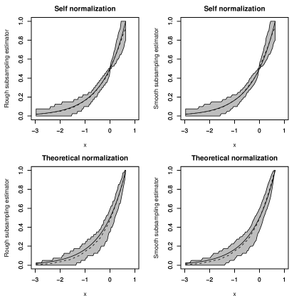
Figure 2: AR(1) process - Monte Carlo approximations to the quantiles ($q_{0.05}$ and $q_{0.95}$) (gray zone) and means (dashed line) of the rough (left) and smooth (right) subsampling estimators computed with the non-overlapping scheme when the normalization coefficients are given by (17) (top) or by (18) (bottom). The asymptotic distribution function, $\mathbb{K}$, is given by the solid line. $n=2,000$, $b=50$, $\epsilon=0.05$.

Finally sequences of length $n=2$,$000$ have also been simulated from the LARCH model with Rademacher iid inputs (2) and with inputs that have a parabolic density probability function given by $x\mapsto 0.5(1+\rho)|x|^{\rho}$ for $x\in\left[-1,1\right]$. Note that the Rademacher distribution can be seen as the limit of the parabolic distribution as $\rho$ goes to infinity. We choose $a=0.4$. Hence the process is weak dependent but not strong mixing when the inputs have a Rademacher distribution, and it is strong mixing when the distribution of the inputs is absolutely continuous. Neither the stationary distribution, nor the extremal behavior of the processes are known. Note however that the end points of the stationary distributions are finite.

We perform simulations and use our estimators. Results are given in Figure 4. The shapes of the empirical distribution functions given by the estimators are different for the two processes (in particular for the large values of $x$). As far as we can see, the generalized extreme value distribution with a negative index could be a good choice to model the distribution of the maximum of the process with absolutely continuous inputs but not to model the distribution of the maximum of the process with Rademacher inputs. The study of the extremal behavior of these processes are intricate and left for future work.

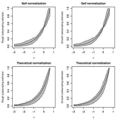
Figure 3: AR(1) process - Monte Carlo approximations to the quantiles ($q_{0.05}$ and $q_{0.95}$) (gray zone) and means (dashed line) of the rough (left) and smooth (right) subsampling estimators computed with the overlapping scheme when the normalization coefficients are given by (17) (top) or by (18) (bottom). The asymptotic distribution function, $\mathbb{K}$, is given by the solid line. $n=2,000$, $b=50$, $\epsilon=0.05$.

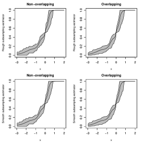
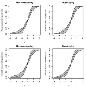
Figure 4: LARCH processes with Rademacher inputs (the four graphs at left) and with parabolic inputs ($\rho=4$) (the four graphs at right) - Monte Carlo approximations to the quantiles ($q_{0.05}$ and $q_{0.95}$) (gray zone) and means (solid line) of the rough (top) and smooth (bottom) subsampling estimators computed with the non-overlapping scheme (left) and with the overlapping scheme (right). $n=2,000$, $b=50$, $\epsilon=0.05$.

6 Proofs

6.1 Proofs for smooth subsampling

A bound of the expression $\widetilde{\Delta}_{b,n}^{(p)}(x)$ is closely related to the coefficients defined for $1\leq q\leq p$ as:

$$C_{b,q}(r)=\sup\left|\mbox{Cov}\,\left(Z_{i_{1}}\cdots Z_{i_{k}},Z_{i_{k+1}}\cdots Z_{i_{q}}\right)\right|$$

where the supremum refers to such indices with $1\leq k<q$, $i_{1}\leq\cdots\leq i_{q}$ satisfy $i_{k+1}-i_{k}=r$ and $Z_{i}=\varphi\left(\frac{s_{b}(Y_{b,i})-x}{\epsilon_{n}}\right)-\mathbb{E}\varphi\left(\frac{s_{b}(Y_{b,i})-x}{\epsilon_{n}}\right)$ is a centered rv. Then setting

$$A_{b,q}(N)=\frac{1}{N^{q}}\sum_{1\leq i_{1}\leq\cdots\leq i_{q}\leq N}\left|\mathbb{E}Z_{i_{1}}\cdots Z_{i_{q}}\right|,\qquad 2\leq q\leq p$$

Doukhan and Louhichi (1999) prove that $\displaystyle\widetilde{\Delta}_{b,n}^{(p)}(x)\leq p!A_{b,p}(N)$, moreover:

$$A_{b,p}(N) \leq B_{b,p}(N)+\sum_{q=2}^{p-2}A_{b,q}(N)A_{b,p-q}(N)$$

$$B_{b,q}(N) = \frac{q-1}{N^{q-1}}\sum_{r=0}^{N-1}(r+1)^{q-2}C_{b,q}(r),\qquad 2\leq q\leq p$$

Lemma 1

Let $p,q,b,N$ be integers and $\beta(b,N)\leq 1$, we assume that for all $2\leq q\leq p$ there exists a constant $c_{q}\geq 0$ such that $B_{b,q}(N)\leq c_{q}\beta^{\frac{q}{2}}(b,N)$. Then there exists a constant $C_{p}\geq 0$ only depending on $p$ and $c_{1},\dots,c_{p}$ such that $A_{b,p}(N)\leq C_{p}\beta^{[\frac{p}{2}]}(b,N)$.

Proof of the lemma 1

The result is the assumption if $p=2$ because $A_{b,2}(N)\leq B_{b,2}(N)$. If now the result has been proved for each $q<p$ the relation $[\frac{p}{2}]\leq[\frac{q}{2}]+[\frac{p-q}{2}]$ completes the proof because $\beta(b,N)\leq 1$.

A covariance $\mbox{Cov}\,\big{(}f(Y_{i_{1}},\ldots,Y_{i_{u}}),g(Y_{j_{1}},\ldots,Y_{j_{v}})\big{)}$ writes respectively as

$$\left\{\begin{array}[]{lr}\mbox{Cov}\,\Big{(}f_{b}\left(\left(X_{i_{h}+k}\right)_{{\tiny\left\{\begin{array}[]{l}1\leq h\leq u\\ 1\leq k\leq b\end{array}\right.}}\right),&g_{b}\left(\left(X_{j_{h^{\prime}}+k^{\prime}}\right)_{{\tiny\left\{\begin{array}[]{l}1\leq h^{\prime}\leq u\\ 1\leq k^{\prime}\leq b\end{array}\right.}}\right)\Big{)}\\ \mbox{Cov}\,\Big{(}f_{b}\left(\left(X_{(i_{h}-1)b+k}\right)_{{\tiny\left\{\begin{array}[]{l}1\leq h\leq u\\ 1\leq k\leq b\end{array}\right.}}\right),&g_{b}\left(\left(X_{(j_{h^{\prime}}-1)b+k^{\prime}}\right)_{{\tiny\left\{\begin{array}[]{l}1\leq h^{\prime}\leq u\\ 1\leq k^{\prime}\leq b\end{array}\right.}}\right)\Big{)}\end{array}\right.$$

for suitable functions $f_{b},g_{b}$ depending if the considered setting is the overlapping one or not. Moreover ${\mathrm{Lip}\,}f_{b}\leq{\mathrm{Lip}\,}f$ which proves that if the dependence coefficients relative to the sequences ${\ X}=(X_{i})_{i\in\mathbb{Z}}$ are denoted by $\eta_{X}(r)=\eta(r)$ and $\eta_{Y_{b}}(r)$, then we get the elementary lemma

Lemma 2 (Heredity)

Assume that the stationary sequence ${X}=(X_{i})_{i\in\mathbb{Z}}$ is weakly dependent then the same occurs for ${Y_{b}}=(Y_{i})_{i\in\mathbb{Z}}$ and:

• $\eta_{Y_{b}}(r)\leq b\eta(r-b)$ if $r\geq b$ in the overlapping case,

• $\lambda_{Y_{b}}(r)\leq b^{2}\lambda(r-b)$ if $r\geq b$ in the overlapping case,

• $\eta_{Y_{b}}(r)\leq b\eta((r-1)b)$ if $r\geq 1$ in the non-overlapping case,

• $\lambda_{Y_{b}}(r)\leq b^{2}\lambda((r-1)b)$ if $r\geq 1$ in the non-overlapping case.

In our setting we use the function $\displaystyle f(y_{1},\ldots,y_{b})=\varphi\left(\frac{s_{b}(y_{1},\ldots,y_{b})-x}{\epsilon_{n}}\right)$, the covariance inequalities write here as:

Lemma 3

Using conditions (5,6) and under the respective weak dependence assumptions $\eta$ and $\lambda$ we respectively get

• in the overlapping case, $C_{b,q}(r)\prec 1$ for $r<b$ and else, resp.

  $$C_{b,q}(r)\prec\frac{bL(b)}{\epsilon_{n}}\eta(r-b),\mbox{ or }C_{b,q}(r)\prec\frac{bL(b)}{\epsilon_{n}}\left(1\vee\frac{bL(b)}{\epsilon_{n}}\right)\lambda(r-b)$$

• in the non-overlapping case, $C_{b,q}(r)\prec 1$ for $r=0$ and else, resp.

  $$C_{b,q}(r)\prec\frac{bL(b)}{\epsilon_{n}}\eta((r-1)b),\mbox{ or }C_{b,q}(r)\prec\frac{bL(b)}{\epsilon_{n}}\left(1\vee\frac{bL(b)}{\epsilon_{n}}\right)\lambda((r-1)b)$$

This lemma entails the bounds:

• Overlapping and $\eta$-dependent case. We obtain

$$B_{b,q}(N) \prec \frac{1}{N^{q-1}}\sum_{r=0}^{b-1}(r+1)^{q-2}+\frac{1}{N^{q-1}}\frac{bL(b)}{\epsilon_{n}}\sum_{r=b}^{N-1}\frac{\eta(r-b)}{(r+1)^{2-q}}$$

$$\prec \left(\frac{b}{N}\right)^{q-1}\left(1+\frac{L(b)}{\epsilon_{n}}\sum_{t=0}^{N-b-1}\eta(t)\right)+\frac{1}{N^{q-1}}\frac{bL(b)}{\epsilon_{n}}\sum_{t=0}^{N-b-1}\frac{\eta(t)}{(t+1)^{2-q}}$$

where the second inequality follows from the change in variable $r=t+b$. We use here $N=n$. Now if we assume $b\prec n^{1-\delta}$ we deduce that $(b/n)^{q-1}\prec n^{-\frac{q}{2}\delta}$ and if $bL(b)\prec n^{1-\delta}\epsilon_{n}$ we analogously derive that $(b/N)^{q-1}(L(b)/\epsilon_{n})\prec n^{-\frac{q}{2}\delta}$. Assume now that

$$\frac{b}{n}\left(1\vee\frac{L(b)}{\epsilon_{n}}\right)\prec n^{-\delta}$$

this implies with $\displaystyle\sum_{t=0}^{\infty}\left(t+1\right)^{q-2}\eta(t)<\infty$ that $B_{b,q}(N)\prec n^{-\frac{q}{2}\delta}$.

• Overlapping and $\lambda$-dependent case. We obtain

$$B_{b,q}(N) \prec \frac{1}{N^{q-1}}\sum_{r=0}^{b-1}(r+1)^{q-2}+\frac{1}{N^{q-1}}\frac{bL(b)}{\epsilon_{n}}\sum_{r=b}^{N-1}\frac{\lambda(r-b)}{(r+1)^{2-q}}$$

$$+\,\frac{1}{N^{q-1}}\frac{(bL(b))^{2}}{\epsilon_{n}^{2}}\sum_{r=b}^{N-1}\frac{\lambda(r-b)}{(r+1)^{2-q}}$$

$$\prec \left(\frac{b}{N}\right)^{q-1}\Bigl{(}1+\frac{L(b)}{\epsilon_{n}}\sum_{t=0}^{N-b-1}\lambda(t)+\frac{bL(b)^{2}}{\epsilon_{n}^{2}}\sum_{t=0}^{N-b-1}\lambda(t)\Bigr{)}$$

$$+\,\frac{1}{N^{q-1}}\left(\frac{bL(b)}{\epsilon_{n}}\sum_{t=0}^{N-b-1}\frac{\lambda(t)}{(t+1)^{2-q}}+\frac{(bL(b))^{2}}{\epsilon_{n}^{2}}\sum_{t=0}^{N-b-1}\frac{\lambda(t)}{(t+1)^{2-q}}\right)$$

where the second inequality follows from the change in variable $r=t+b$. We use here $N=n$. Now if we assume $b\prec n^{1-\delta}$ we deduce that $(b/n)^{q-1}\prec n^{-\frac{q}{2}\delta}$. Now if $(bL(b)\vee(bL(b))^{2})\prec n^{1-\delta}(\epsilon_{n}\vee\epsilon_{n}^{2})$ we analogously derive that $(b/N)^{q-1}(L(b)/\epsilon_{n}\vee bL(b)^{2}/\epsilon_{n}^{2})\prec n^{-\frac{q}{2}\delta}$. Assume now that

$$\frac{b}{n}\left(1\vee\frac{L(b)}{\epsilon_{n}}\vee\frac{bL(b)^{2}}{\epsilon_{n}^{2}}\right)\prec n^{-\delta}$$

this implies with $\displaystyle\sum_{t=0}^{\infty}\left(t+1\right)^{q-2}\lambda(t)<\infty$ that $B_{b,q}(N)\prec n^{-\frac{q}{2}\delta}$.

• Non-overlapping and $\eta$-dependent case. We obtain

$$B_{b,q}(N) \prec \frac{1}{N^{q-1}}+\frac{1}{N^{q-1}}\frac{bL(b)}{\epsilon_{n}}\sum_{r=1}^{N-1}\frac{\eta((r-1)b)}{(r+1)^{2-q}}$$

$$\prec \frac{1}{N^{q-1}}\Bigl{(}1+\frac{bL(b)}{\epsilon_{n}}\sum_{k=1}^{n-1}\eta(k)\Bigr{)}+\frac{1}{N^{q-1}}\frac{b^{3-q}L(b)}{\epsilon_{n}}\sum_{k=1}^{n-1}\frac{\eta(k)}{k^{2-q}}$$

where the second inequality follows from replacement of $k=b(r-1)$. We use here $N=n/b$. Now if we assume $b\prec n^{1-\delta}$ we deduce that $(b/n)^{q-1}\prec n^{-\frac{q}{2}\delta}$ and if $b^{2}L(b)\prec n^{1-\delta}\epsilon_{n}$ we analogously derive that $(1/N^{q-1})(bL(b)/\epsilon_{n})\prec n^{-\frac{q}{2}\delta}$. Assume now that

$$\frac{b}{n}\left(1\vee\frac{bL(b)}{\epsilon_{n}}\right)\prec n^{-\delta}$$

this implies with $\displaystyle\sum_{t=0}^{n-1}\left(t+1\right)^{q-2}\eta(t)<b^{q-2}$ that $B_{b,q}(N)\prec n^{-\frac{q}{2}\delta}$.

• Non-overlapping and $\lambda$-dependent case. We obtain

$$B_{b,q}(N) \prec \frac{1}{N^{q-1}}+\frac{1}{N^{q-1}}\frac{bL(b)}{\epsilon_{n}}\sum_{r=b}^{N-1}\frac{\lambda((r-1)b)}{(r+1)^{2-q}}+\frac{1}{N^{q-1}}\frac{(bL(b))^{2}}{\epsilon_{n}^{2}}\sum_{r=b}^{N-1}\frac{\lambda((r-1)b)}{(r+1)^{2-q}}$$

$$\prec \left(\frac{1}{N}\right)^{q-1}\Bigl{(}1+\frac{bL(b)}{\epsilon_{n}}\sum_{k=b}^{n-1}\lambda(k)+\frac{bL(b)^{2}}{\epsilon_{n}^{2}}\sum_{k=b}^{n-1}\lambda(k)\Bigr{)}$$

$$+\,\frac{1}{N^{q-1}}\left(\frac{b^{3-q}L(b)}{\epsilon_{n}}\sum_{k=b}^{n-1}\frac{\lambda(k)}{k^{2-q}}+\frac{b^{5-q}L(b)^{2}}{\epsilon_{n}^{2}}\sum_{k=b}^{n-1}\frac{\lambda(k)}{k^{2-q}}\right),$$

where the second inequality follows from replacement of $k=b(r-1)$. We use here $N=n/b$. Now if we assume $b\prec n^{1-\delta}$ we deduce that $(b/n)^{q-1}\prec n^{-\frac{q}{2}\delta}$. Now if $(b^{2}L(b)\vee(bL(b))^{2})\prec n^{1-\delta}(\epsilon_{n}\vee\epsilon_{n}^{2})$ we analogously derive that $(1/N^{q-1})(bL(b)/\epsilon_{n}\vee bL(b)^{2}/\epsilon_{n}^{2})\prec n^{-\frac{q}{2}\delta}$. Assume now that

$$\frac{b}{n}\left(1\vee\frac{bL(b)}{\epsilon_{n}}\vee\frac{bL(b)^{2}}{\epsilon_{n}^{2}}\right)\prec n^{-\delta}$$

this implies with $\displaystyle\sum_{t=0}^{n-1}\left(t+1\right)^{q-2}\lambda(t)<\left(b^{q-2}\vee b^{q-4}\right)$ that $B_{b,q}(N)\prec n^{-\frac{q}{2}\delta}$.

Lemma 4

The relation $B_{b,q}(N)\prec n^{-\frac{q}{2}\delta}$ holds in the following cases

• In the overlapping case, if we have respectively

  $$\sum_{t=0}^{\infty}(t+1)^{q-2}\eta(t)<\infty,\mbox{ and } \frac{b}{n}\left(1\vee\frac{L(b)}{\epsilon_{n}}\right)\prec n^{-\delta},\qquad\qquad\quad\qquad\qquad\quad$$

  $$\sum_{t=0}^{\infty}(t+1)^{q-2}\lambda(t)<\infty,\mbox{ and } \frac{b}{n}\left(1\vee\frac{L(b)}{\epsilon_{n}}\vee\frac{bL(b)^{2}}{\epsilon_{n}^{2}}\right)\prec n^{-\delta}.$$

• In the non-overlapping case, if we have respectively

  $$\sum_{t=0}^{n-1}(t+1)^{q-2}\eta(t)<b^{q-2},\mbox{ and } \frac{b}{n}\left(1\vee\frac{bL(b)}{\epsilon_{n}}\right)\prec n^{-\delta},\qquad\qquad\quad\qquad\qquad$$

  $$\sum_{t=0}^{n-1}(t+1)^{q-2}\lambda(t)<\left(b^{q-2}\vee b^{q-4}\right),\mbox{and} \frac{b}{n}\left(1\vee\frac{bL(b)}{\epsilon_{n}}\vee\frac{bL(b)^{2}}{\epsilon_{n}^{2}}\right)\prec n^{-\delta}.$$

This lemma together with lemma 1 yields the main theorem.

6.2 Proofs for rough subsampling

In this section we shall replace $\epsilon_{n}$ by some $z>0$ to be settled later and we set $\varphi_{z}(t)=\varphi\left(\frac{t-x}{z}\right)$. We now set $Z_{i}=\mbox{I1}_{\{s_{b}(Y_{b,i})\leq x\}}-\mathbb{P}(s_{b}(Y_{b,i})\leq x)$ and $W_{i}=\varphi_{z}(s_{b}(Y_{b,i}))-\mathbb{E}\varphi_{z}(s_{b}(Y_{b,i}))$. An usual trick yields:

$$\left|\mbox{Cov}\,\left(Z_{i_{1}}\cdots Z_{i_{k}},Z_{i_{k+1}}\cdots Z_{i_{q}}\right)\right| \leq \left|\mbox{Cov}\,\left(W_{i_{1}}\cdots W_{i_{k}},W_{i_{k+1}}\cdots W_{i_{q}}\right)\right|$$

$$+ 2\sum_{h=1}^{p}\mathbb{E}|W_{i_{h}}-Z_{i_{h}}|\,=\,U+V$$

with $U=\left|\mbox{Cov}\,\left(W_{i_{1}}\cdots W_{i_{k}},W_{i_{k+1}}\cdots W_{i_{q}}\right)\right|$ and $V=2p\,\mathbb{P}(s_{b}(Y_{b,i})\in[x,x+z])$.
A bound for $V$ does not depend on the overlapping or not overlapping case and we get

$$\left\{\begin{array}[]{llllll}V&\leq&2p(G{\mathrm{Lip}\,}s_{b}z+r_{b})&\prec&L(b)z+r_{b},&\mbox{under assumption }(\ref{con})\\ V&\leq&2pC(b)z^{c}&\prec&C(b)z^{c},&\mbox{ under assumption }(\ref{conc})\end{array}\right.$$

Set here $A_{p,b,\epsilon}={bp{\mathrm{Lip}\,}s_{b}}/z\prec bL(b)/z$. The bound of $U$ needs 4 cases (considered in Lemma 3) with

• in the overlapping case, $\displaystyle U\prec\left\{\begin{array}[]{ll}\frac{bL(b)}{z}\eta(r-b),&\mbox{for }r\geq b\\ 1,&\mbox{for }r<b\end{array}\right.$

• in the overlapping case, $\displaystyle U\prec\left\{\begin{array}[]{ll}\frac{bL(b)}{z}(1\vee\frac{bL(b)}{z})\lambda(r-b),&\mbox{for }r\geq b\\ 1,&\mbox{for }r<b\end{array}\right.$

• in the non-overlapping case, $\displaystyle U\prec\left\{\begin{array}[]{ll}\frac{bL(b)}{z}\eta((r-1)b),&\mbox{for }r\geq 1\\ 1,&\mbox{for }r=0\end{array}\right.$

• in the non-overlapping case, $\displaystyle U\prec\left\{\begin{array}[]{ll}\frac{bL(b)}{z}(1\vee\frac{bL(b)}{z})\lambda((r-1)b),&\mbox{for }r\geq 1\\ 1,&\mbox{for }r=0\end{array}\right.$

We first derive the inequality $(t+1+b)^{q-2}\leq 2^{(q-3)}\vee 1\left\{(t+1)^{q-2}+b^{q-2}\right\}$ from convexity if $q>3$ and sublinearity else, thus:

$$(t+1+b)^{q-2}\prec(t+1)^{q-2}+b^{q-2}.$$

Coefficients $C_{b,q}(r)\prec\sup\{U+V\}$ may thus be bounded in all the considered cases.

For simplicity we classify the cases with couples of numbers indicating the fact overlapping (5) or not (6) setting is used and from the fact the convergence (3) or concentration (3) is assumed, which makes 4 different cases to consider). Consider the cases under assumption (3).

- $\eta$ (5,3) case. Note that

$$C_{b,q}(r) \prec L(b)\Bigl{(}b\eta(r-b)/z+z\Bigr{)}+r_{b}\prec L(b)\sqrt{b\eta(r-b)}+r_{b}\qquad\qquad\qquad$$

with the choice $z=\sqrt{b\eta(r-b)}$. This yields

$$B_{b,q}(N) \prec \frac{1}{N^{q-1}}\sum_{r=0}^{b-1}(r+1)^{q-2}+\frac{L(b)\sqrt{b}}{N^{q-1}}\sum_{r=b}^{N-1}\frac{\sqrt{\eta(r-b)}}{(r+1)^{2-q}}+r_{b}$$

$$\prec \left(\frac{b}{N}\right)^{q-1}\Bigl{(}1+\frac{L(b)}{\sqrt{b}}\sum_{t=0}^{N-b-1}\sqrt{\eta(t)}\Bigr{)}+\frac{L(b)\sqrt{b}}{N^{q-1}}\sum_{t=0}^{N-b-1}\frac{\sqrt{\eta(t)}}{(t+1)^{2-q}}$$

$$+\,r_{b},$$

where the second inequality follows from the change in variable $r=t+b$. We use here $N=n$. Now if we assume that $b\prec n^{1-\delta}$, we deduce that $(b/n)^{q-1}\prec n^{-q\delta/2}$ and if $bL(b)\prec n^{1-\delta}$ we analogously derive that $(b/N)^{q-1}(L(b)/\sqrt{b})\prec n^{-\frac{q}{2}\delta}$. If $\eta(t)\prec n^{-\eta}$ and $\sigma\leq\eta/2$ we assume that

$$\frac{b}{n}\left(1\vee\frac{L(b)}{\sqrt{b}}\right)+r_{b}\prec n^{-\delta},\qquad\sum_{t=0}^{\infty}(t+1)^{q-2}\eta(t)^{1/2}<\infty.$$

- $\eta$ (6,3) case. Note that

$$C_{b,q}(r) \prec bL(b)\eta((r-1)b)/z+L(b)z+r_{b}\prec L(b)\sqrt{b\eta((r-1)b)}+r_{b}$$

where we use $z=\sqrt{b\eta((r-1)b)}$, then

$$B_{b,q}(N) \prec \frac{1}{N^{q-1}}+\frac{L(b)\sqrt{b}}{N^{q-1}}\sum_{r=1}^{N-1}\frac{\sqrt{\eta((r-1)b)}}{(r+1)^{2-q}}+r_{b}$$

$$\prec \frac{1}{N^{q-1}}\Bigl{(}1+L(b)\sqrt{b}\sum_{k=b}^{n-1}\sqrt{\eta(k)}\Bigr{)}+\frac{L(b)b^{\frac{5}{2}-q}}{N^{q-1}}\sum_{k=b}^{n-1}\frac{\sqrt{\eta(k)}}{k^{2-q}}+r_{b}\!\!\!$$

where the second inequality follows from replacement of $k=b(r-1)$. We use here $N=n/b$. Let us assume $b\prec n^{1-\delta}$, then we deduce that $(b/n)^{q-1}\prec n^{-\frac{q}{2}\delta}$ and if $b^{3/2}L(b)\prec n^{1-\delta}$ we analogously derive that $(1/N)^{q-1}(L(b)\sqrt{b})\prec n^{-\frac{q}{2}\delta}$. If $\eta(t)\prec n^{-\eta}$ and $\sigma\leq\eta/2$ we assume that

$$\frac{b}{n}\left(1\vee\sqrt{b}L(b)\right)+r_{b}\prec n^{-\delta},\qquad\sum_{t=0}^{\infty}\eta(t)^{1/2}<\infty.$$

- $\lambda$ (5,3) case. Note that

$$C_{b,q}(r) \prec L(b)z+\left(bL(b)/z+\left(bL(b)/z\right)^{2}\right)\lambda(r-b)+r_{b}$$

$$\prec 2(bL(b)^{2})^{\frac{2}{3}}\lambda(r-b)^{\frac{1}{3}}+(bL(b)^{2})^{\frac{1}{3}}\lambda(r-b)^{\frac{2}{3}}+r_{b},$$

with a choice $z=(b^{2}L(b)\lambda(r-b))^{\frac{1}{3}}$. Then

$$B_{b,q}(N) \prec \frac{1}{N^{q-1}}\sum_{r=0}^{b-1}(r+1)^{q-2}+\frac{2(bL(b)^{2})^{\frac{2}{3}}}{N^{q-1}}\sum_{r=b}^{N-1}\frac{\lambda(r-b)^{\frac{1}{3}}}{(r+1)^{2-q}}$$

$$+\,\frac{(bL(b)^{2})^{\frac{1}{3}}}{N^{q-1}}\sum_{r=b}^{N-1}\frac{\lambda(r-b)^{\frac{2}{3}}}{(r+1)^{2-q}}+r_{b}$$

$$\prec \left(\frac{b}{N}\right)^{q-1}\left(1+(b^{-1}L(b)^{4})^{\frac{1}{3}}\sum_{t=0}^{N-b-1}\lambda(t)^{\frac{1}{3}}+(b^{-1}L(b))^{\frac{2}{3}}\sum_{t=0}^{N-b-1}\lambda(t)^{\frac{2}{3}}\right)$$

$$+\,\frac{1}{N^{q-1}}\left((bL(b)^{2})^{\frac{2}{3}}\sum_{t=0}^{N-b-1}\frac{\lambda(t)^{\frac{1}{3}}}{(t+1)^{2-q}}+(bL(b)^{2})^{\frac{1}{3}}\sum_{t=0}^{N-b-1}\frac{\lambda(t)^{\frac{2}{3}}}{(t+1)^{2-q}}\right)$$

$$+\,r_{b}$$

where the second inequality follows from the change in variable $r=t+b$. We use here $N=n$. Let us assume $b\prec n^{1-\delta}$, then we deduce that $(b/n)^{q-1}\prec n^{-\frac{q}{2}\delta}$ and if $\left((bL(b)^{2})^{2/3}\vee(bL(b)^{2})^{1/3}\right)\prec n^{1-\delta}$ we analogously derive that $(b/N)^{q-1}\left((b^{-1}L(b)^{4})^{\frac{1}{3}}\vee(b^{-1}L(b))^{\frac{2}{3}}\right)\prec n^{-\frac{q}{2}\delta}$. If $\lambda(t)\prec n^{-\lambda}$ and $\sigma\leq\lambda/2$ and $\sigma\leq 2\lambda/3$ we assume that

$$\frac{b}{n}\left(1\vee(b^{-1}L(b)^{4})^{\frac{1}{3}}\vee(b^{-1}L(b))^{\frac{2}{3}}\right)+r_{b}\prec n^{-\delta}$$

with $\displaystyle\sum_{t=0}^{\infty}(t+1)^{q-2}\lambda(t)^{1/3}<\infty$ and $\displaystyle\sum_{t=0}^{\infty}(t+1)^{q-2}\lambda(t)^{2/3}<\infty$.

- $\lambda$ (6,3) case. Note that

$$C_{b,q}(r) \prec \left(L(b)z+r_{b}\right)+\left(\frac{bL(b)}{z}+\left(\frac{bL(b)}{z}\right)^{2}\right)\lambda((r-1)b)$$

$$\prec 2(bL(b)^{2})^{\frac{2}{3}}\lambda((r-1)b)^{\frac{1}{3}}+(bL(b)^{2})^{\frac{1}{3}}\lambda((r-1)b)^{\frac{2}{3}}+r_{b},$$

with a choice $z=(b^{2}L(b)\lambda((r-1)b))^{\frac{1}{3}}$. Then we obtain

$$B_{b,q}(N) \prec \frac{1}{N^{q-1}}+\frac{(bL(b)^{2})^{\frac{2}{3}}}{N^{q-1}}\sum_{r=1}^{N-1}(r+1)^{q-2}\lambda((r-1)b)^{\frac{1}{3}}$$

$$+\,\frac{(bL(b)^{2})^{\frac{1}{3}}}{N^{q-1}}\sum_{r=1}^{N-1}(r+1)^{q-2}\lambda((r-1)b)^{\frac{2}{3}}+r_{b}$$

$$\prec \frac{1}{N^{q-1}}\Bigl{(}1+(bL(b)^{2})^{\frac{2}{3}}\sum_{k=1}^{n-1}\lambda(k)^{\frac{1}{3}}+(bL(b)^{2})^{\frac{1}{3}}\sum_{k=1}^{n-1}\lambda(k)^{\frac{2}{3}}\Bigr{)}$$

$$+\,\frac{1}{N^{q-1}}\Bigl{(}L(b)^{\frac{4}{3}}b^{\frac{8}{3}-q}\sum_{k=1}^{n-1}\frac{\lambda(k)^{\frac{1}{3}}}{k^{2-q}}+L(b)^{\frac{2}{3}}b^{\frac{7}{3}-q}\sum_{k=1}^{n-1}\frac{\lambda(k)^{\frac{2}{3}}}{k^{2-q}}\Bigr{)}+r_{b}$$

where the second inequality follows from the change in variable $k=b(r-1)$. We use here $N=n/b$. Let us assume $b\prec n^{1-\delta}$, then we deduce that $(b/n)^{q-1}\prec n^{-\frac{q}{2}\delta}$ and if $\left(b^{\frac{5}{3}}L(b)^{\frac{4}{3}}\vee b^{\frac{4}{3}}L(b)^{\frac{2}{3}}\right)\prec n^{1-\delta}$ then we analogously derive that $(b/n)^{q-1}\left((bL(b)^{2})^{\frac{2}{3}}\vee(bL(b)^{2})^{\frac{1}{3}}\right)\prec n^{-\frac{q}{2}\delta}$. If $\lambda(t)\prec n^{-\lambda}$ and $\sigma\leq\lambda/3$ and $\sigma\leq 2\lambda/3$ we assume that

$$\frac{b}{n}\left((bL(b)^{2})^{\frac{2}{3}}\vee(bL(b)^{2})^{\frac{1}{3}}\right)+r_{b}\prec n^{-\delta}$$

with $\displaystyle\sum_{t=0}^{n-1}(t+1)^{q-2}\lambda(t)^{1/3}<\infty$ and $\displaystyle\sum_{t=0}^{n-1}(t+1)^{q-2}\lambda(t)^{2/3}<\infty$ that bound holds.
Consider now the cases under assumption (3).
- $\eta$ (5,3) case. Note that

$$C_{b,q}(r) \prec L(b)b\eta(r-b)/z+C(b)z^{c}\qquad\qquad\qquad\qquad\qquad\qquad\qquad\qquad$$

$$\prec \Bigl{(}C(b)(bL(b)\eta(r-b))^{c}\Bigr{)}^{\frac{1}{1+c}}+\Bigl{(}bL(b)\eta(r-b)\Bigr{)}^{\frac{2+c}{1+c}}$$

with a choice $z=(bL(b)\eta(r-b)/C(b))^{\frac{1}{c+1}}$, then

$$B_{b,q}(N)$$

$$\prec \frac{1}{N^{q-1}}\sum_{r=0}^{b-1}(r+1)^{q-2}+\frac{\left(C(b)(bL(b))^{c}\right)^{\frac{1}{1+c}}}{N^{q-1}}\sum_{r=b}^{N-1}(r+1)^{q-2}(\eta(r-b))^{\frac{c}{1+c}}$$

$$+\frac{\left(bL(b)\right)^{\frac{2+c}{1+c}}}{N^{q-1}}\sum_{r=b}^{N-1}(r+1)^{q-2}(\eta(r-b))^{\frac{2+c}{1+c}}$$

$$\prec \left(\frac{b}{N}\right)^{q-1}\Bigl{(}1+\left(C(b)b^{-1}L(b)^{c}\right)^{\frac{1}{1+c}}\sum_{t=0}^{N-b-1}\eta(t)^{\frac{c}{1+c}}+\left(bL(b)^{2+c}\right)^{\frac{1}{1+c}}\sum_{t=0}^{N-b-1}\eta(t)^{\frac{2+c}{1+c}}\Bigr{)}$$

$$+\,\frac{1}{N^{q-1}}\Bigl{(}\left(C(b)(bL(b))^{c}\right)^{\frac{1}{1+c}}\sum_{t=0}^{N-b-1}\frac{\eta(t)^{\frac{c}{1+c}}}{(t+1)^{2-q}}+\left(bL(b)\right)^{\frac{2+c}{1+c}}\sum_{t=0}^{N-b-1}\frac{\eta(t)^{\frac{2+c}{1+c}}}{(t+1)^{2-q}}\Bigr{)}$$

where the second inequality follows from the change in variable $r=t+b$. We use here $N=n$. Now if we assume $b\prec n^{1-\delta}$ we deduce that $(b/n)^{q-1}\prec n^{-\frac{q}{2}\delta}$ and if $b\left((C(b)b^{-1}L(b)^{c})^{\frac{1}{1+c}}\vee(bL(b)^{2+c})^{\frac{2+c}{1+c}}\right)\prec n^{1-\delta}$ we analogously derive $(b/N)^{q-1}\left((C(b)b^{-1}L(b)^{c})^{\frac{1}{1+c}}\vee(bL(b)^{2+c})^{\frac{2+c}{1+c}}\right)\prec n^{-\frac{q}{2}\delta}.$
If $\eta(t)\prec n^{-\eta}$ and $\sigma\leq\eta\frac{c}{1+c}$ and $\sigma\leq\eta\frac{2+c}{1+c}$ we assume that

$$\frac{b}{n}\left(1\vee\left(C(b)b^{-1}L(b)^{c}\right)^{\frac{1}{1+c}}\vee\left(bL(b)^{2+c}\right)^{\frac{1}{1+c}}\right)\prec n^{-\delta}$$

which implies with $\displaystyle\sum_{t=0}^{\infty}\left(t+1\right)^{q-2}\eta(t)^{\frac{c}{1+c}}<b^{q-2}$ and $\displaystyle\sum_{t=0}^{\infty}\left(t+1\right)^{q-2}\eta(t)^{\frac{2+c}{1+c}}<b^{q-2}$ that $B_{b,q}(N)\prec n^{-\frac{q}{2}\delta}.$
- $\eta$ (6,3) case. Note that

$$C_{b,q}(r) \prec L(b)b\eta((r-1)b)/z+C(b)z^{c}\qquad\qquad\qquad\qquad\qquad\qquad\qquad\qquad\qquad\qquad\qquad\qquad$$

$$\prec (C(b)(bL(b)\eta((r-1)b))^{c}))^{\frac{1}{1+c}}+(bL(b)\eta((r-1)b))^{\frac{2+c}{1+c}}$$

with a choice $z=(bL(b)\eta((r-1)b)/C(b))^{\frac{1}{c+1}}$. Then

$$B_{b,q}(N)$$

$$\prec \frac{1}{N^{q-1}}+\frac{\left(C(b)(bL(b))^{c}\right)^{\frac{1}{1+c}}}{N^{q-1}}\sum_{r=1}^{N-1}(r+1)^{q-2}\eta((r-1)b)^{\frac{c}{1+c}}$$

$$+\,\frac{(bL(b))^{\frac{2+c}{1+c}}}{N^{q-1}}\sum_{r=1}^{N-1}(r+1)^{q-2}\eta((r-1)b)^{\frac{2+c}{1+c}}$$

$$\prec \frac{1}{N^{q-1}}\Bigl{(}1+\left(C(b)(bL(b))^{c}\right)^{\frac{1}{1+c}}\sum_{k=b}^{n-1}\eta(k)^{\frac{c}{1+c}}+(bL(b))^{\frac{2+c}{1+c}}\sum_{k=b}^{n-1}\eta(k)^{\frac{2+c}{1+c}}\Bigr{)}$$

$$+\,\frac{1}{N^{q-1}}\Bigl{(}\left(C(b)L(b)^{c}\right)^{\frac{1}{1+c}}b^{\frac{2+3c}{1+c}-q}\sum_{k=b}^{n-1}\frac{\eta(k)^{\frac{c}{1+c}}}{k^{2-q}}$$

$$+\,L(b)^{\frac{2+c}{1+c}}b^{\frac{4+3c}{1+c}-q}\sum_{k=b}^{n-1}\frac{\eta(k)^{\frac{2+c}{1+c}}}{k^{2-q}}\Bigr{)}$$

where the second inequality folllows from the change in variables $k=b(r-1)$. We use here $N=n/b$. Now if we assume $b\prec n^{1-\delta}$, we deduce that $(b/n)^{q-1}\prec n^{-\frac{q}{2}\delta}$. Now if $\left(1\vee(C(b)(bL(b))^{c})^{\frac{1}{1+c}}\vee(bL(b))^{\frac{2+c}{1+c}}\right)\prec n^{-\delta}$ we analogously derive $(1/N)^{q-1}\left(1\vee(C(b)(bL(b))^{c})^{\frac{1}{1+c}}\vee(bL(b))^{\frac{2+c}{1+c}}\right)\prec n^{-\frac{q}{2}\delta}$. If $\eta(t)\prec n^{-\eta}$ and $\sigma\leq\eta\frac{c}{1+c}$ and $\sigma\leq\eta\frac{2+c}{1+c}$ we assume that

$$\frac{b}{n}\left(1\vee(C(b)(bL(b))^{c})^{\frac{1}{1+c}}\vee(bL(b))^{\frac{2+c}{1+c}}\right)\prec n^{-\delta}$$

which implies with $\displaystyle\sum_{t=0}^{n-1}\left(t+1\right)^{q-2}\eta(t)^{\frac{c}{1+c}}\prec b^{q-2}$ and $\displaystyle\sum_{t=0}^{n-1}\left(t+1\right)^{q-2}\eta(t)^{\frac{2+c}{1+c}}\prec b^{q-2}$ that $B_{b,q}(N)\prec n^{-\frac{q}{2}\delta}.$
- $\lambda$ (5,3) case. Note that

$$C_{b,q}(r) \prec C(b)z^{c}+\left(bL(b)/z+\left(bL(b)/z\right)^{2}\right)\lambda(r-b),$$

$$\prec (C(b)bL(b)^{c})^{\frac{2}{2+c}}(\lambda(r-b))^{\frac{c}{2+c}}+\left(C(b)(bL(b)^{c})^{\frac{1}{2+c}}\right)(\lambda(r-b))^{\frac{1+c}{2+c}}$$

$$+\,\left(C(b)(bL(b)^{2c})^{\frac{1}{2+c}}\right)(\lambda(r-b))^{\frac{1+c}{2+c}},$$

with a choice $z=((bL(b))^{2}C(b)^{-1}\lambda(r-b))^{\frac{1}{2+c}}$.

$$B_{b,q}(N)$$

$$\prec \frac{1}{N^{q-1}}\sum_{r=0}^{b-1}(r+1)^{q-2}+\frac{(C(b)(bL(b))^{c})^{\frac{2}{2+c}}}{N^{q-1}}\sum_{r=b}^{N-1}\frac{\lambda(r-b)^{\frac{c}{2+c}}}{(r+1)^{2-q}}$$

$$+\,\frac{(C(b)(bL(b))^{c})^{\frac{1}{2+c}}}{N^{q-1}}\sum_{r=b}^{N-1}\frac{\lambda(r-b)^{\frac{1+c}{2+c}}}{(r+1)^{2-q}}+\frac{(C(b)(bL(b))^{2c})^{\frac{1}{2+c}}}{N^{q-1}}\sum_{r=b}^{N-1}\frac{\lambda(r-b)^{\frac{1+c}{2+c}}}{(r+1)^{2-q}}$$

$$\prec \left(\frac{b}{N}\right)^{q-1}\Bigr{(}1+(C(b)^{2}b^{c-2}L(b)^{2c})^{\frac{1}{2+c}}\sum_{t=0}^{N-b-1}\lambda(t)^{\frac{c}{2+c}}$$

$$+\,(C(b)b^{-2}L(b)^{c})^{\frac{1}{2+c}}\sum_{t=0}^{N-b-1}\lambda(t)^{\frac{1+c}{2+c}}+(C(b)b^{c-2}L(b)^{2c})^{\frac{1}{2+c}}\sum_{t=0}^{N-b-1}\lambda(t)^{\frac{1+c}{2+c}}\Bigl{)}$$

$$+\,\frac{1}{N^{q-1}}\Bigl{(}(C(b)(bL(b))^{c})^{\frac{2}{2+c}}\sum_{t=0}^{N-b-1}\frac{\lambda(t)^{\frac{c}{2+c}}}{(t+1)^{2-q}}+(C(b)(bL(b))^{c})^{\frac{1}{2+c}}\sum_{t=0}^{N-b-1}\frac{\lambda(t)^{\frac{1+c}{2+c}}}{(t+1)^{2-q}}$$

$$+\,(C(b)(bL(b))^{2c})^{\frac{1}{2+c}}\sum_{t=0}^{N-b-1}\frac{\lambda(t)^{\frac{1+c}{2+c}}}{(t+1)^{2-q}}\Bigr{)}$$

where the second inequality follows from the change in variable $r=t+b$. We use here $N=n$. Now if we assume that $b\prec n^{1-\delta}$ we deduce that $(b/n)^{q-1}\prec n^{-\frac{q}{2}\delta}$.
If $b\left((C(b)^{2}b^{c-2}L(b)^{2c})^{\frac{1}{2+c}}\vee(C(b)b^{-2}L(b)^{c})^{\frac{1}{2+c}}\vee(C(b)b^{c-2}L(b)^{2c})^{\frac{1}{2+c}}\right)\prec n^{1-\delta}$ we analogously derive

$$(b/N)^{q-1}\left((C(b)^{2}b^{c-2}L(b)^{2c})^{\frac{1}{2+c}}\vee(C(b)b^{-2}L(b)^{c})^{\frac{1}{2+c}}\vee(C(b)b^{c-2}L(b)^{2c})^{\frac{1}{2+c}}\right)\prec n^{-\frac{q}{2}\delta}.$$

If $\lambda(t)\prec n^{-\lambda}$ and $\sigma\leq\lambda\frac{c}{1+c}$ and $\sigma\leq\lambda\frac{2+c}{1+c}$ we assume that

$$\frac{b}{n}\left(1\vee(C(b)^{2}b^{c-2}L(b)^{2c})^{\frac{1}{2+c}}\vee(C(b)b^{-2}L(b)^{c})^{\frac{1}{2+c}}\vee(C(b)b^{c-2}L(b)^{2c})^{\frac{1}{2+c}}\right)\prec n^{-\delta}$$

which implies with $\displaystyle\sum_{t=0}^{\infty}\left(t+1\right)^{q-2}\lambda(t)^{\frac{c}{1+c}}<b^{q-2}$ and $\displaystyle\sum_{t=0}^{\infty}\left(t+1\right)^{q-2}\lambda(t)^{\frac{2+c}{1+c}}<b^{q-2}$ that $B_{b,q}(N)\prec n^{-\frac{q}{2}\delta}.$
- $\lambda$ (6,3) case. Note that

$$C_{b,q}(r) \prec C(b)z^{c}+\left(\frac{bL(b)}{z}+\left(\frac{bL(b)}{z}\right)^{2}\right)\lambda((r-1)b)$$

$$\prec (C(b)(bL(b))^{c})^{\frac{2}{2+c}}\lambda((r-1)b)^{\frac{c}{2+c}}+\left((C(b)(bL(b))^{c})^{\frac{1}{2+c}}\right)\lambda((r-1)b)^{\frac{1+c}{2+c}}$$

$$+\,\left((C(b)(bL(b))^{2c})^{\frac{1}{2+c}}\right)\lambda((r-1)b)^{\frac{1+c}{2+c}},$$

with a choice $z=((bL(b))^{2}C(b)^{-1}\lambda((r-1)b))^{\frac{1}{2+c}}$. We obtain

$$B_{b,q}(N) \prec \frac{1}{N^{q-1}}+\frac{(C(b)(bL(b))^{c})^{\frac{2}{2+c}}}{N^{q-1}}\sum_{r=1}^{N-1}(r+1)^{q-2}\lambda((r-1)b)^{\frac{c}{2+c}}$$

$$+\,\frac{(C(b)(bL(b))^{c})^{\frac{1}{2+c}}}{N^{q-1}}\sum_{r=1}^{N-1}(r+1)^{q-2}\lambda((r-1)b)^{\frac{1+c}{2+c}}$$

$$+\,\frac{(C(b)(bL(b))^{2c})^{\frac{1}{2+c}}}{N^{q-1}}\sum_{r=1}^{N-1}(r+1)^{q-2}\lambda((r-1)b)^{\frac{1+c}{2+c}}$$

$$\prec \frac{1}{N^{q-1}}\Bigr{(}1+(C(b)(bL(b))^{c})^{\frac{2}{2+c}}\sum_{k=1}^{n-1}\lambda(k)^{\frac{c}{2+c}}+(C(b)(bL(b))^{c})^{\frac{1}{2+c}}\sum_{k=1}^{n-1}\lambda(k)^{\frac{1+c}{2+c}}$$

$$+\,(C(b)(bL(b))^{2c})^{\frac{1}{2+c}}\sum_{k=1}^{n-1}\lambda(k)^{\frac{1+c}{2+c}}\Bigl{)}+\frac{1}{N^{q-1}}\Bigr{(}(C(b)L(b)^{c})^{\frac{2}{2+c}}b^{\frac{4(1+c)}{2+c}-q}\sum_{k=1}^{n-1}\frac{\lambda(k)^{\frac{c}{2+c}}}{k^{2-q}}$$

$$+\,(C(b)L(b)^{c})^{\frac{1}{2+c}}b^{\frac{4+3c}{2+c}-q}\sum_{k=1}^{n-1}\frac{\lambda(k)^{\frac{1+c}{2+c}}}{k^{2-q}}+(C(b)L(b)^{2c})^{\frac{1}{2+c}}b^{\frac{4(1+c)}{2+c}-q}\sum_{k=1}^{n-1}\frac{\lambda(k)^{\frac{1+c}{2+c}}}{k^{2-q}}\Bigr{)}$$

where the second inequality follows from the change in variable $k=b(r-1)$. We use here $N=n/b$. Now if we assume that $b\prec n^{1-\delta}$ we deduce that $(b/n)^{q-1}\prec n^{-\frac{q}{2}\delta}$.
If $b\left((C(b)(bL(b))^{c})^{\frac{2}{2+c}}\vee(C(b)(bL(b))^{c})^{\frac{1}{2+c}}\vee\vee(C(b)(bL(b))^{2c})^{\frac{1}{2+c}}\right)\prec n^{1-\delta}$ we analogously derive that
$(b/N)^{q-1}\left((C(b)(bL(b))^{c})^{\frac{2}{2+c}}\vee(C(b)(bL(b))^{c})^{\frac{1}{2+c}}\vee(C(b)(bL(b))^{2c})^{\frac{1}{2+c}}\right)\prec n^{-\frac{q}{2}\delta}$. If $\lambda(t)\prec n^{-\lambda}$ and $\sigma\leq\lambda\frac{c}{1+c}$ and $\sigma\leq\lambda\frac{2+c}{1+c}$ we assume that

$$\frac{b}{n}\left(1\vee(C(b)(bL(b))^{c})^{\frac{2}{2+c}}\vee(C(b)(bL(b))^{c})^{\frac{1}{2+c}}\vee(C(b)(bL(b))^{2c})^{\frac{1}{2+c}}\right)\prec n^{-\delta}$$

which implies with $\displaystyle\sum_{t=0}^{n-1}(t+1)^{q-2}\lambda(t)^{\frac{c}{1+c}}\prec b^{q-2}$ and $\displaystyle\sum_{t=0}^{n-1}(t+1)^{q-2}\lambda(t)^{\frac{2+c}{1+c}}\prec b^{q-2}$ that $B_{b,q}(N)\prec n^{-\frac{q}{2}\delta}.$

Lemma 5

The relation $\widehat{\Delta}_{b,n}^{(2)}(x)\rightarrow_{n\rightarrow\infty}0$ holds in the following cases under the convergence assumption (3)

• In the overlapping case, if we have respectively

  $$\sum_{t=0}^{\infty}\eta(t)^{1/2}<\infty,\mbox{and} r_{b}+\frac{b}{n}\left(1\vee\frac{L(b)}{\sqrt{b}}\right)\to 0,\qquad\qquad\quad,$$

  $$\sum_{t=0}^{\infty}\lambda(t)^{2/3}<\infty,\mbox{and} r_{b}+\frac{b}{n}\left(1\vee\left(\frac{L(b)^{4}}{b}\right)^{1/3}\vee\left(\frac{L(b)}{b}\right)^{2/3}\right)\to 0.$$

• In the non-overlapping case, if we have respectively

  $$\sum_{t=0}^{\infty}\eta(t)^{1/2}<\infty, r_{b}+\frac{b}{n}\left(1\vee\sqrt{b}L(b)\right)\to 0,$$ and

  $$\sum_{t=0}^{\infty}\lambda(t)^{2/3}<\infty, r_{b}+\frac{b}{n}\left(1\vee(bL(b)^{2})^{2/3}\vee(bL(b)^{2})^{1/3}\right)\to 0.$$ and

This lemma together with lemma 1 yields theorem 2.

Lemma 6

The relation $B_{b,q}(N)\prec n^{-q\delta/2}$ holds under concentration assumption (3) if respectively the overlapping setting is used and one among the following relations hold as $n\rightarrow\infty$

$$\eta\mbox{-dependence:}\sum_{t=0}^{\infty}(t+1)^{q-2}\eta(t)^{\frac{2+c}{1+c}}<\infty,\qquad\qquad\qquad\qquad\qquad\qquad\qquad\qquad\qquad$$

$$\frac{b}{n}\left(1\vee\left(C(b)b^{-1}L(b)^{c}\right)^{\frac{1}{1+c}}\vee\left(bL(b)^{2+c}\right)^{\frac{1}{1+c}}\right)\prec n^{-\delta},$$

$$\lambda\mbox{-dependence:}\sum_{t=0}^{\infty}(t+1)^{q-2}\lambda(t)^{\frac{1+c}{2+c}}<\infty,\mbox{ }\qquad\qquad\qquad\qquad\qquad\qquad\qquad\qquad\qquad$$

$$\frac{b}{n}\left(1\vee(C(b)^{2}b^{c-2}L(b)^{2c})^{\frac{1}{2+c}}\vee(C(b)b^{-2}L(b)^{c})^{\frac{1}{2+c}}\vee(C(b)b^{c-2}L(b)^{2c})^{\frac{1}{2+c}}\right)\prec n^{-\delta}$$

or the non-overlapping setting is used and

$$\eta\mbox{-dependence:}\sum_{t=0}^{n-1}(t+1)^{q-2}\eta(t)^{\frac{2+c}{1+c}}\prec b^{q-2},\qquad\qquad\qquad\qquad\qquad\qquad\qquad\qquad\qquad$$

$$\frac{b}{n}\left(1\vee\left(C(b)(bL(b))^{c}\right)^{\frac{1}{1+c}}\vee(bL(b))^{\frac{2+c}{1+c}}\right)\prec n^{-\delta},$$

$$\lambda\mbox{-dependence:}\sum_{t=0}^{n-1}(t+1)^{q-2}\lambda(t)^{\frac{1+c}{2+c}}\prec b^{q-2},\qquad\qquad\qquad\qquad\qquad\qquad\qquad\qquad\qquad$$

$$\frac{b}{n}\left(1\vee(C(b)(bL(b))^{c})^{\frac{2}{2+c}}\vee(C(b)(bL(b))^{c})^{\frac{1}{2+c}}\vee(C(b)(bL(b))^{2c})^{\frac{1}{2+c}}\right)\prec n^{-\delta}.$$

This lemma together with lemma 1 yields theorem 3.

6.3 Proof of Theorem 5

Put $k_{n}=\left\lfloor n/a_{n}\right\rfloor$. Partition $\{1,\ldots,n\}$ into $k_{n}$ blocks of size $a_{n}$

$$J_{j}=J_{j,n}=\left\{\left(j-1\right)a_{n}+1,\ldots,ja_{n}\right\},\qquad j=1,\ldots,k_{n},$$

and, in case $k_{n}a_{n}<n$, a remainder block, $J_{k_{n}+1}=\left\{k_{n}a_{n}+1,\ldots,n\right\}$. Observe that

$$\mathbb{P}(M_{n}\leq w_{n}(x))=\mathbb{P}\left(\bigcap_{j=1}^{k_{n}+1}\left\{M\left(J_{j}\right)\leq w_{n}(x)\right\}\right)$$

where $M\left(J_{j}\right)=\max_{i\in J_{j}}(X_{i})$. Since $\mathbb{P}(M\left(J_{j}\right)>w_{n}(x))\leq a_{n}\bar{F}\left(w_{n}(x)\right)\rightarrow 0$ as $n\rightarrow\infty$, the remainder block can be omitted and

$$\mathbb{P}(M_{n}\leq w_{n}(x))=\mathbb{P}\left(\bigcap_{j=1}^{k_{n}}\left\{M\left(J_{j}\right)\leq w_{n}(x)\right\}\right)+o\left(1\right).$$

Let

$$J_{j}^{\ast} = J_{j,n}^{\ast}=\left\{\left(j-1\right)a_{n}+1,\ldots,ja_{n}-l_{n}\right\},\qquad j=1,\ldots,k_{n},$$

$$J_{j}^{\prime} = J_{j,n}^{\prime}=\left\{ja_{n}-l_{n},\ldots,ja_{n}\right\},\qquad j=1,\ldots,k_{n}.$$

Since $P\left(\bigcup_{j=1}^{k_{n}}M\left(J_{j}^{\prime}\right)>w_{n}(x)\right)\leq k_{n}l_{n}\bar{F}\left(w_{n}(x)\right)\rightarrow 0$ as $n\rightarrow\infty$, we deduce that

$$\mathbb{P}(M_{n}\leq w_{n}(x))=\mathbb{P}\left(\bigcap_{j=1}^{k_{n}}\left\{M\left(J_{j}^{\ast}\right)\leq w_{n}(x)\right\}\right)+o\left(1\right).$$

Let $B_{j}=B_{j,n}=\left\{M\left(J_{j}^{\ast}\right)\leq w_{n}(x)\right\}$. We write

$$\mathbb{P}\left(\bigcap_{j=1}^{k_{n}}B_{j}\right)-\prod_{j=1}^{k_{n}}\mathbb{P}(B_{j})$$

$$= \sum_{i=1}^{k_{n}}\left(\mathbb{P}\left(\bigcap_{j=1}^{k_{n}-i+1}B_{j}\right)\prod_{j=k_{n}-i+2}^{k_{n}}\mathbb{P}(B_{j})-\mathbb{P}\left(\bigcap_{j=1}^{k_{n}-i}B_{j}\right)\prod_{j=k_{n}-i+1}^{k_{n}}\mathbb{P}(B_{j})\right)$$

$$= \sum_{i=1}^{k_{n}}\left(\mathbb{P}\left(\bigcap_{j=1}^{k_{n}-i+1}B_{j}\right)-\mathbb{P}\left(\bigcap_{j=1}^{k_{n}-i}B_{j}\right)\mathbb{P}(B_{k_{n}-i+1})\right)\prod_{j=k_{n}-i+2}^{k_{n}}\mathbb{P}(B_{j}).$$

We want to bound the following quantity

$$\left|\mathbb{P}\left(\bigcap_{j=1}^{k_{n}-i+1}B_{j}\right)-\mathbb{P}\left(\bigcap_{j=1}^{k_{n}-i}B_{j}\right)\mathbb{P}(B_{k_{n}-i+1})\right|.$$

Let us define $f_{n}^{\left(x\right)}(y)=\mathbb{I}_{\{y\leq w_{n}(x)\}}$. Let $(\alpha_{n})$ be a sequence such that $\alpha_{n}\rightarrow 0$ as $n\rightarrow\infty$ and put $x_{n}^{-}=x-\alpha_{n}$ and $x_{n}^{+}=x+\alpha_{n}$. We simply approximate the function $f_{n}^{\left(x\right)}$ by Lipschitz and bounded functions $g_{n},h_{n}\in\mathcal{F}_{1}$ with

$$f_{n}^{(x_{n}^{-})}\leq g_{n}\leq f_{n}^{\left(x\right)}\leq h_{n}\leq f_{n}^{(x_{n}^{+})}$$

and we quote that it is easy to choose functions $g_{n}$ and $h_{n}$ with Lipschitz coefficient $u_{n}\alpha_{n}^{-1}$. For $I\subset\{1,\ldots,n\}$, let $H_{I}(f_{n}^{\left(x\right)})=\mathbb{E}\left[\prod_{i\in I}f_{n}^{\left(x\right)}(X_{i})\right]$. Note that

$$H_{I}(f_{n}^{\left(x_{n}^{-}\right)})\leq H_{I}(g_{n})\leq H_{I}(f_{n}^{\left(x\right)})\leq H_{I}(h_{n})\leq H_{I}(f_{n}^{\left(x_{n}^{+}\right)}).$$

Let $C_{I,J}(f_{n}^{\left(x\right)})=H_{I\cup J}(f_{n}^{\left(x\right)})-H_{I}(f_{n}^{\left(x\right)})H_{J}(f_{n}^{\left(x\right)})$, we have

$$C_{I,J}(g_{n})-\delta_{I,J}\left(g_{n},h_{n}\right)\leq C_{I,J}(f_{n}^{\left(x\right)})\leq C_{I,J}(h_{n})+\delta_{I,J}\left(g_{n},h_{n}\right)$$

with

$$\delta_{I,J}\left(g_{n},h_{n}\right)=H_{I}(h_{n})H_{J}(h_{n})-H_{I}(g_{n})H_{J}(g_{n}).$$

Let $I_{i}=\left\{l:\{X_{l}\leq w_{n}(x)\}\in\bigcap_{j=1}^{k_{n}-i}B_{j}\right\}$ and $J_{i}=\left\{l:\{X_{l}\leq w_{n}(x)\}\in B_{k_{n}-i+1}\right\}$. We have

$$\left|H_{I_{i}}(h_{n})-H_{I_{i}}(g_{n})\right| \leq \left(k_{n}-i+1\right)a_{n}\left(\bar{F}(w_{n}(x_{n}^{-}))-\bar{F}(w_{n}(x_{n}^{+}))\right)$$

$$\left|H_{J_{i}}(h_{n})-H_{J_{i}}(g_{n})\right| \leq a_{n}\left(\bar{F}(w_{n}(x_{n}^{-}))-\bar{F}(w_{n}(x_{n}^{+}))\right)$$

Then we have

$$\left|C_{I_{i},J_{i}}(f_{n}^{\left(x\right)})\right|\leq\left|C_{I_{i},J_{i}}(h_{n})\right|\vee\left|C_{I_{i},J_{i}}(g_{n})\right|+|\delta_{I_{i},J_{i}}\left(g_{n},h_{n}\right)|$$

and

$$|\delta_{I_{i},J_{i}}\left(g_{n},h_{n}\right)|\leq\left|H_{I_{i}}(h_{n})-H_{I_{i}}(g_{n})\right|+\left|H_{J_{i}}(h_{n})-H_{J_{i}}(g_{n})\right|.$$

Note that as $n\rightarrow\infty$

$$n\left(\bar{F}(w_{n}(x_{n}^{-}))-\bar{F}(w_{n}(x_{n}^{+}))\right)\sim 2\alpha_{n}\gamma(1+\gamma x)_{+}^{-1/\gamma-1}.$$

If $X$ is $\eta$-weakly dependent, it follows that

$$\left|C_{I_{i},J_{i}}(f_{n}^{\left(x\right)})\right|\leq\left(k_{n}-i+2\right)a_{n}u_{n}\alpha_{n}^{-1}\eta(l_{n})+2\alpha_{n}\gamma(1+\gamma x)_{+}^{-1/\gamma-1}\frac{\left(k_{n}-i+2\right)a_{n}}{n}.$$

An optimal choice of $\alpha_{n}$ is then given by

$$\alpha_{n}\sim\left[n\eta(l_{n})u_{n}\right]^{1/2}$$

and then

$$\left|C_{I_{i},J_{i}}(f_{n}^{\left(x\right)})\right|\prec\left(n\eta(l_{n})u_{n}\right)^{1/2}.$$

It follows that

$$\left|\mathbb{P}\left(\bigcap_{j=1}^{k_{n}}B_{j}\right)-\prod_{j=1}^{k_{n}}\mathbb{P}(B_{j})\right|\prec k_{n}\left(n\eta(l_{n})u_{n}\right)^{1/2}.$$

If $X$ is $\lambda$-weakly dependent, it follows that

$$\left|C_{I_{i},J_{i}}(f_{n}^{\left(x\right)})\right| \leq \left[\left(k_{n}-i+2\right)a_{n}u_{n}\alpha_{n}^{-1}+\left(k_{n}-i+1\right)a_{n}u_{n}^{2}\alpha_{n}^{-2}\right]\lambda(l_{n})$$

$$+2\alpha_{n}\gamma(1+\gamma x)_{+}^{-1/\gamma-1}\frac{\left(k_{n}-i+2\right)a_{n}}{n}.$$

An optimal choice of $\alpha_{n}$ is then given by

$$\alpha_{n}\sim\left[k_{n}\lambda(l_{n})u_{n}\right]^{1/2}\vee\left[k_{n}\lambda(l_{n})u_{n}^{2}\right]^{1/3}$$

and then

$$\left|C_{I_{i},J_{i}}(f_{n}^{\left(x\right)})\right|\prec(\left[n\lambda(l_{n})u_{n}\right]^{1/2}\vee\left[na_{n}\lambda(l_{n})u_{n}^{2}\right]^{1/3}).$$

It follows that

$$\left|\mathbb{P}\left(\bigcap_{j=1}^{k_{n}}B_{j}\right)-\prod_{j=1}^{k_{n}}\mathbb{P}(B_{j})\right|\prec k_{n}(\left[n\lambda(l_{n})u_{n}\right]^{1/2}\vee\left[na_{n}\lambda(l_{n})u_{n}^{2}\right]^{1/3}).$$

Finally we deduce that

$$\mathbb{P}(M_{n}\leq w_{n}\left(x\right))=\left[\mathbb{P}(M_{n}\leq w_{a_{n}}\left(x\right))\right]^{k_{n}}+o(1)$$

and the result follows.

Aknowledgements.

We want to thank Patrice Bertail for essential discussions during many years at ENSAE. The first author also wants to thank Paul Embrechts at ETHZ and the Swiss Banking Institute at Zurich University for their strong support.

Paul DOUKHAN (doukhan@u-cergy.fr)

University Cergy Pontoise, UFR Sciences-Techniques, Saint-Martin

2, avenue Adolphe-Chauvin, B.P. 222 Pontoise

95302 Cergy-Pontoise cedex

France

Silika PROHL (prohl@isb.uzh.ch)

Swiss Institute for International Economics and Applied Economic Research

Zurich University

Switzerland

Christian Y. ROBERT (chrobert@ensae.fr)

Ecole Nationale de la Statistique et de l’Administration Economique

Timbre J120, 3 Avenue Pierre Larousse

92245 Malakoff Cedex

France

References

- [1] Andrews, D. (1984) Non strong mixing autoregressive processes. Journal of Applied Probability 21, 930–934.
- [2] Ango Nze, P., Doukhan, P. (2004) Weak dependence and applications to econometrics. Econometric Theory 20, 995?-1045.
- [3] Bertail, P., Haefke, C., Politis, D. N., White, W. (2004) Subsampling the distribution of diverging statistics with applications to finance. Journal of Econometrics 120, 295–326.
- [4] Bickel, P. J., Wichura, M. J. (1971) Convergence criteria for multiparameter stochastic processes and some applications. Ann. Math. Stat. 42, 1656–1670.
- [5] Bradley, R. (2007) Introduction to strong mixing conditions. Volumes 1,2 and 3. Kendricks Press.
- [6] Chernick, M. (1981) A limit theorem for the maximum of autoregressive processes with uniform marginal distribution. Annals of Probability 9, 145–149.
- [7] Dedecker, J., Doukhan, P. (2003) A new covariance inequality and applications. Stoch. Proc. Appl. 106-1, 63–80.
- [8] Dedecker, J., Doukhan, P., Lang, G., León, J. R., Louhichi, S. , Prieur, C. (2007) Weak dependence: models, theory and applications. Lecture Notes in Statistics 190, Springer-Verlag, New-York.
- [9] Doukhan, P. (1994) Mixing: properties and examples. Lecture Notes in Statistics 85, Springer-Verlag, New-York.
- [10] Doukhan, P., Louhichi, S. (1999) A new weak dependence condition and applications to moment inequalities. Stoch. Proc. Appl. 84, 313–342.
- [11] Doukhan, P., Madre, H., Rosenbaum, M. (2007) Weak dependence for infinite ARCH-type bilinear models. Statistics 41, 31–45.
- [12] Doukhan, P., Mayo, N., Truquet, L. (2009) Weak dependence, models and some applications. Metrika 69 2-3, 199–225.
- [13] Doukhan, P., Wintenberger, O. (2007) An invariance principle for weakly dependent stationary general models. Probability and Mathematical Statistics 27, 45–73.
- [14] Doukhan, P., Wintenberger, O. (2008) Weakly dependent chains with infinite memory. Stochastic Process Appl. 118, 1997–2013.
- [15] Engle, R. F. (1982) Autoregressive conditional heteroskedasticity with estimate of the variance in the U.K. inflation. Econometrica 15, 286–301.
- [16] Leadbetter, M. R. (1974). On extreme values in stationary sequences. Z. Wahr. Ver. Geb. 28, 289–303.
- [17] Leadbetter, M. R. (1983). Extremes and local dependence in stationary sequences. Z. Wahr. Ver. Geb. 65, 291–306.
- [18] Leadbetter, M. R., Lindgren, G., Rootzen, H. (1983) Extremes and related properties of random sequences and processes. Springer Series in Statistics.
- [19] O’Brien, G. L. (1987). Extreme values for stationary and Markov sequences. Ann. Probab. 15, 281–291.
- [20] Perfekt, R. (1994) Extremal behavior of stationary Markov chains with applications. Ann. Appl. Probab. 4-2, 529–542.
- [21] Petrov, V. (1995) Limit theorems of probability theory. Clarendon Press, Oxford.
- [22] Politis, D. N., Romano, J. P. (1994) Large sample confidence regions based on subsamples under minimal assumptions. Annals of Statistics 22, 2031–2050.
- [23] Rio, E. (2000) Théorie asymptotique pour des processus aléatoires faiblement dépendants. SMAI, Mathématiques et Applications 31, Springer.