A log-Birnbaum–Saunders Regression Model with Asymmetric Errors

Abstract

The paper by Leiva et al. (2010) introduced a skewed version of the sinh-normal distribution, discussed some of its properties and characterized an extension of the Birnbaum–Saunders distribution associated with this distribution. In this paper, we introduce a skewed log-Birnbaum–Saunders regression model based on the skewed sinh-normal distribution. Some influence methods, such as the local influence and generalized leverage are presented. Additionally, we derived the normal curvatures of local influence under some perturbation schemes. An empirical application to a real data set is presented in order to illustrate the usefulness of the proposed model.

Key words: Birnbaum–Saunders distribution; fatigue life distribution; influence diagnostic; maximum likelihood estimators; sinh-normal distribution; skew-normal distribution.

1 Introduction

The two-parameter Birnbaum-Saunders (BS) distribution, also known as the fatigue life distribution, was introduced by Birnbaum and Saunders (1969a, b). It was originally derived from a model for a physical fatigue process where dominant crack growth causes failure. A more general derivation was provided by Desmond (1985) based on a biological model and relaxing several of the assumptions made by Birnbaum and Saunders (1969a). Desmond (1986) investigated the relationship between the BS distribution and the inverse Gaussian distribution. The author established that the BS distribution can be written as a mixture equally weighted from an inverse Gaussian distribution and its complementary reciprocal.

The random variable $T$ is said to have a BS distribution with parameters $\alpha,\eta>0$, say ${\rm BS}(\alpha,\eta)$, if its cumulative distribution function (cdf) is given by $F(t)=\Phi(v)$, $t>0$, where $\Phi(\cdot)$ is the standard normal distribution function, $v=\rho(t/\eta)/\alpha$, $\rho(z)=z^{1/2}-z^{-1/2}$ and $\alpha$ and $\eta$ are shape and scale parameters, respectively. Also, $\eta$ is the median of the distribution: $F(\eta)=\Phi(0)=1/2$. For any constant $k>0$, it follows that $kT\sim{\rm BS}(\alpha,k\eta)$. It is noteworthy that the reciprocal property holds for the BS distribution: $T^{-1}\sim{\rm BS}(\alpha,\eta^{-1})$; see Saunders (1974). The BS distribution has received considerable attention over the last few years. Kundu et al. (2008) discussed the shape of the hazard function of the BS distribution. Results on improved statistical inference for the BS distribution are discussed in Wu and Wong (2004) and Lemonte et al. (2007, 2008). Some generalizations and extensions of the BS distribution are presented in Díaz–García and Leiva (2005), Gómes et al. (2009), Guiraud et al. (2009) and Castillo et al. (2009). This distribution has been applied in reliability studies (see, for example, Balakrishnan et al., 2007) and outside this field; see Leiva et al. (2008) and Leiva et al. (2009). Additionally, based on the BS distribution, Bhatti (2010) introduced the BS autoregressive conditional duration model. Xu and Tang (2010) presented estimators for the unknown parameters of the BS distribution using reference prior.

From Rieck (1989), if

$$Z=\nu+\frac{2}{\alpha}\sinh\biggl{(}\frac{Y-\gamma}{\sigma}\biggr{)}\sim{\rm N}(0,1),$$ (1)

then $Y$ has a four-parameter sinh-normal (SHN) distribution, denoted by $Y\sim{\rm SHN}(\alpha,\gamma,\sigma,\nu)$, where $\nu\in\Re$ and $\alpha>0$ are the shape parameters, and $\gamma\in\Re$ and $\sigma>0$ correspond to the location and scale parameters, respectively. According to Rieck (1989), the parameter $\nu$ is also the noncentralty parameter. If $\nu=0$, the notation is reduced simply by $Y\sim{\rm SHN}(\alpha,\gamma,\sigma)$, and this distribution has a number of interesting properties. For example, it is symmetric around the mean ${\rm E}(Y)=\gamma$, it is unimodal for $\alpha\leq 2$ and bimodal for $\alpha>2$ and if $Y_{\alpha}\sim{\rm SHN}(\alpha,\gamma,\sigma)$, then $Z_{\alpha}=2(Y_{\alpha}-\gamma)/(\alpha\sigma)$ converges in distribution to the standard normal distribution when $\alpha\to 0$. If $Y\sim{\rm SHN}(\alpha,\gamma,\sigma=2)$, then $T=\exp(Y)$ follows the BS distribution with shape parameter $\alpha$ and scale parameter $\eta=\exp(\gamma)$, i.e. $T=\exp(Y)\sim{\rm BS}(\alpha,\eta)$. For this reason, according to Leiva et al. (2010), the SHN distribution is also called the log-Birnbaum–Saunders (log-BS) distribution. Additionally, according to these authors, the SHN and BS models corresponding to a logarithmic distribution and its associated distribution, respectively (Marshall and Olkin, 2007, Ch. 12).

Rieck and Nedelman (1991) introduced a log-BS regression model based on the ${\rm SHN}(\alpha,\gamma,2)$ distribution. Their regression model has been studied by several authors. Some important references are Tisionas (2001), Galea et al. (2004), Leiva et al. (2007), Desmond et al. (2008), Lemonte et al. (2010), Xiao et al. (2010) and Cancho et al. (2010), among others. Generalizations of the log-BS regression model introduced by Rieck and Nedelman (1991) are presented in Xi and Wei (2007, § 4) and Lemonte and Cordeiro (2009).

Leiva et al. (2010) introduced a skewed SHN distribution by replacing the standard normal distribution in equation (1) by the skew-normal (SN) distribution (Azzaline, 1985), i.e. they consider the random variable

$$Z=\nu+\frac{2}{\alpha}\sinh\biggl{(}\frac{Y-\gamma}{\sigma}\biggr{)}\sim{\rm SN}(\lambda),$$

where $\lambda\in\Re$ is the shape parameter which determines the skewness. Now, the notation used is $Y\sim{\rm SSN}(\alpha,\gamma,\sigma,\nu,\lambda)$. From now on, we shall consider $\nu=0$ and $\sigma=2$ and hence the notation is given by $Y\sim{\rm SSN}(\alpha,\gamma,2,\lambda)$. The random variable $T=\exp(Y)$ follows the extended Birnbaum–Saundres (EBS) distribution, with shape parameters $\alpha>0$ and $\lambda\in\Re$, and scale parameter $\eta=\exp(\gamma)$. Now, the notation is $T=\exp(Y)\sim{\rm EBS}(\alpha,\eta,\lambda)$.

Let $T\sim{\rm EBS}(\alpha,\eta,\lambda)$. The density function of $Y=\log(T)$ is given by (Leiva et al., 2010)

$$\pi(y)=\frac{2}{\alpha}\cosh\biggl{(}\frac{y-\gamma}{2}\biggr{)}\phi\biggl{(}\frac{2}{\alpha}\sinh\biggl{(}\frac{y-\gamma}{2}\biggr{)}\biggr{)}\Phi\biggl{(}\frac{2\lambda}{\alpha}\sinh\biggl{(}\frac{y-\gamma}{2}\biggr{)}\biggr{)},\qquad y\in\Re,$$

where $\phi(\cdot)$ is the standard normal density function, and, as before, we write $Y\sim{\rm SSN}(\alpha,\gamma,2,\lambda)$. The $s$th ($s=1,2,\ldots$) moment of $Y$ can be written as

$${\rm E}(Y^{s})=2^{k}\sum_{k=0}^{s}\gamma^{s-k}c_{k}(\alpha,\lambda),\qquad c_{k}(\alpha,\lambda)=\int_{-\infty}^{\infty}\{\sinh^{-1}(\alpha w/2)\}^{k}\phi(w)\Phi(\lambda w)dw.$$

Thus, the mean of $Y$ is given by ${\rm E}(Y)=\gamma+c(\alpha,\lambda)$, with

$$c(\alpha,\lambda)=4\int_{-\infty}^{\infty}\{\sinh^{-1}(\alpha w/2)\}\phi(w)\Phi(\lambda w)dw.$$

Plots of the ${\rm SSN}(\alpha,\gamma,2,\lambda)$ distribution are illustrated in Figure 1 for selected parameter values.

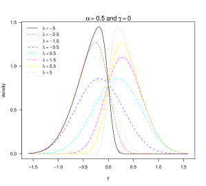
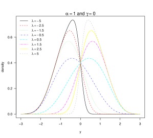
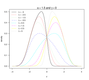
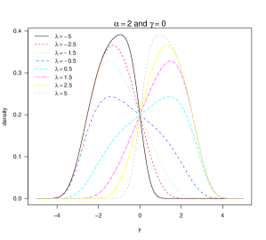
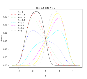
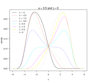
Figure 1: Plots of the density function of the SSN distribution for some parameter values.

The chief goal of this paper is to introduce a skewed log-BS regression model based on the ${\rm SSN}(\alpha,\gamma,2,\lambda)$ distribution, recently proposed by Leiva et al. (2010). The proposed regression model is convenient for modeling asymmetric data, and it is an alternative to the log-BS regression model introduced by Rieck and Nedelman (1991) when the data present skewness. The article is organized as follows. Section 2 introduces the class of skewed log-BS regression models. The score functions and observed information matrix are given. Section 3 deals with some basic calculations related with local influence. Derivations of the normal curvature under different perturbation schemes are presented in Section 4. Generalized leverage is derived in Section 5. Section 6 contains an application to a real data set of the proposed regression model. Finally, concluding remarks are offered in Section 7.

2 Model specification

The skewed log-BS regression model is defined by

$$y_{i}=\bm{x}_{i}^{\top}\bm{\beta}+\varepsilon_{i},\qquad i=1\ldots,n,$$ (2)

where $y_{i}$ is the logarithm of the $i$th observed lifetime, $\bm{x}_{i}=(x_{i1},\ldots,x_{ip})^{\top}$ is a vector of known explanatory variables associated with the $i$th observable response $y_{i}$, $\bm{\beta}=(\beta_{1},\ldots,\beta_{p})^{\top}$ is a vector of unknown parameters, and the random errors $\varepsilon_{i}\sim{\rm SSN}(\alpha,-c(\alpha,\lambda),2,\lambda)$ that corresponds to the regression model where the error distribution has mean zero. Thus, we have $y_{i}\sim{\rm SSN}(\alpha,\bm{x}_{i}^{\top}\bm{\beta}-c(\alpha,\lambda),2,\lambda)$, with ${\rm E}(y_{i})=\bm{x}_{i}^{\top}\bm{\beta}$, for $i=1,\ldots,n$.

The log-likelihood function for the vector parameter $\bm{\theta}=(\bm{\beta}^{\top},\alpha,\lambda)^{\top}$ from a random sample $\bm{y}=(y_{1},\ldots,y_{n})^{\top}$ obtained from (2) can be expressed as

$$\ell(\bm{\theta})=\sum_{i=1}^{n}\ell_{i}(\bm{\theta}),$$ (3)

where $\ell_{i}(\bm{\theta})=-\log(2\pi)/2+\log(\xi_{i1})-\xi_{i2}^{2}/2+\log\{\Phi(\lambda\xi_{i2})\}$,

$$\xi_{i1}=\xi_{i1}(\bm{\theta})=\frac{2}{\alpha}\cosh\biggl{(}\frac{y_{i}-\bm{x}_{i}^{\top}\bm{\beta}+c(\alpha,\lambda)}{2}\biggr{)},\quad\xi_{i2}=\xi_{i2}(\bm{\theta})=\frac{2}{\alpha}\sinh\biggl{(}\frac{y_{i}-\bm{x}_{i}^{\top}\bm{\beta}+c(\alpha,\lambda)}{2}\biggr{)},$$

for $i=1,\ldots,n$. The function $\ell(\bm{\theta})$ is assumed to be regular (Cox and Hinkley, 1974, Ch. 9) with respect to all $\bm{\beta}$, $\alpha$ and $\lambda$ derivatives up to second order. Further, the $n\times p$ matrix $\bm{X}=(\bm{x}_{1},\ldots,\bm{x}_{n})^{\top}$ is assumed to be of full rank, i.e., rank($\bm{X})=p$.

By taking the partial derivatives of the log-likelihood function with respect to $\bm{\beta}$, $\alpha$ and $\lambda$, we obtain the components of the score vector $\bm{U}_{\bm{\theta}}=(\bm{U}_{\bm{\beta}}^{\top},U_{\alpha},U_{\lambda})^{\top}$. We have $\bm{U}_{\bm{\beta}}=\bm{X}^{\top}\bm{s}$, where $\bm{s}=(s_{1},\ldots,s_{n})^{\top}$ with $s_{i}=\{\xi_{i1}\xi_{i2}-\xi_{i2}/\xi_{i1}-\lambda\xi_{i1}\phi(\lambda\xi_{i1})/\Phi(\lambda\xi_{i2})\}/2$,

$$U_{\alpha} =-\frac{n}{\alpha}+\frac{1}{\alpha}\sum_{i=1}^{n}\xi_{i2}^{2}-\frac{c_{\alpha}}{2}\sum_{i=1}^{n}\biggl{\{}\xi_{i1}\xi_{i2}-\frac{\xi_{i2}}{\xi_{i1}}\biggr{\}}$$

$$\quad+\lambda\sum_{i=1}^{n}\frac{\phi(\lambda\xi_{i2})}{\Phi(\lambda\xi_{i2})}\biggl{\{}\frac{c_{\alpha}\xi_{i1}}{2}-\frac{\xi_{i2}}{\alpha}\biggr{\}},$$

$$U_{\lambda}=-\frac{c_{\lambda}}{2}\sum_{i=1}^{n}\biggl{\{}\xi_{i1}\xi_{i2}-\frac{\xi_{i2}}{\xi_{i1}}\biggr{\}}+\frac{1}{2}\sum_{i=1}^{n}\frac{\phi(\lambda\xi_{i2})}{\Phi(\lambda\xi_{i2})}\{\lambda c_{\lambda}\xi_{i1}+2\xi_{i2}\},$$

where

$$c_{\alpha}=c_{\alpha}(\alpha,\lambda)=4\int_{-\infty}^{\infty}w(4+\alpha^{2}w^{2})^{-1/2}\phi(w)\Phi(\lambda w)dw,$$

$$c_{\lambda}=c_{\lambda}(\alpha,\lambda)=4\int_{-\infty}^{\infty}w\sinh^{-1}(\alpha w/2)\phi(w)\Phi(\lambda w)dw.$$

Setting these equations to zero, $\bm{U}_{\bm{\theta}}=\bm{0}$, and solving them simultaneously yields the MLE $\widehat{\bm{\theta}}=(\widehat{\bm{\beta}}^{\top},\widehat{\alpha},\widehat{\lambda})^{\top}$ of $\bm{\theta}=(\bm{\beta}^{\top},\alpha,\lambda)^{\top}$. These equations cannot be solved analytically and statistical software can be used to solve them numerically. For example, the BFGS method (see, Nocedal and Wright, 1999; Press et al., 2007) with analytical derivatives can be used for maximizing the log-likelihood function $\ell(\bm{\theta})$. Starting values $\bm{\beta}^{(0)}$, $\alpha^{(0)}$ and $\lambda^{(0)}$ are required. Our suggestion is to use as an initial point estimate for $\bm{\beta}$ the ordinary least squares estimate of this parameter vector, that is, $\bar{\bm{\beta}}=(\bm{X}^{\top}\bm{X})^{-1}\bm{X}^{\top}\bm{y}$. The initial guess for $\alpha$ we suggest is $\sqrt{\bar{\alpha}^{2}}$, where

$$\bar{\alpha}^{2}=\frac{4}{n}\sum_{i=1}^{n}\sinh^{2}\biggr{(}\frac{y_{i}-\bm{x}_{i}^{\top}\bar{\bm{\beta}}}{2}\biggl{)}.$$

We suggest $\lambda^{(0)}=0$. These initial guesses worked well in the application described in Section 6.

The asymptotic inference for the parameter vector $\bm{\theta}=(\bm{\beta}^{\top},\alpha,\lambda)^{\top}$ can be based on the normal approximation of the MLE of $\bm{\theta}$, $\widehat{\bm{\theta}}=(\widehat{\bm{\beta}}^{\top},\widehat{\alpha},\widehat{\lambda})^{\top}$. Under some regular conditions stated in Cox and Hinkley (1974, Ch. 9) that are fulfilled for the parameters in the interior of the parameter space, we have $\widehat{\bm{\theta}}\stackrel{{\scriptstyle a}}{{\sim}}\mathcal{N}_{p+2}(\bm{\theta},\bm{\Sigma}_{\bm{\theta}})$, for $n$ large, where $\stackrel{{\scriptstyle a}}{{\sim}}$ means approximately distributed and $\bm{\Sigma}_{\bm{\theta}}$ is the asymptotic variance-covariance matrix for $\widehat{\bm{\theta}}$. The asymptotic behavior remains valid if $\bm{\Sigma}_{\bm{\theta}}$ is approximated by $-\ddot{\bm{L}}_{\widehat{\bm{\theta}}\widehat{\bm{\theta}}}^{-1}$, where $-\ddot{\bm{L}}_{\widehat{\bm{\theta}}\widehat{\bm{\theta}}}$ is the $(p+2)\times(p+2)$ observed information matrix evaluated at $\widehat{\bm{\theta}}$, obtained from

$$\ddot{\bm{L}}_{\bm{\theta}\bm{\theta}}=\begin{bmatrix}\ddot{\bm{L}}_{\bm{\beta}\bm{\beta}}&\ddot{\bm{L}}_{\bm{\beta}\alpha}&\ddot{\bm{L}}_{\bm{\beta}\lambda}\\ \ddot{\bm{L}}_{\alpha\bm{\beta}}&\ddot{L}_{\alpha\alpha}&\ddot{L}_{\alpha\lambda}\\ \ddot{\bm{L}}_{\lambda\bm{\beta}}&\ddot{L}_{\lambda\alpha}&\ddot{L}_{\lambda\lambda}\end{bmatrix}=\begin{bmatrix}-\bm{X}^{\top}\bm{V}\bm{X}&-\bm{X}^{\top}\bm{h}&-\bm{X}^{\top}\bm{b}\\ -\bm{h}^{\top}\bm{X}&{\rm tr}(\bm{K}_{1})&{\rm tr}(\bm{K}_{2})\\ -\bm{b}^{\top}\bm{X}&{\rm tr}(\bm{K}_{2})&{\rm tr}(\bm{K}_{3})\end{bmatrix},$$

where

$$\bm{V}={\rm diag}\{v_{1},\ldots,v_{n}\},\qquad\bm{K}_{1}={\rm diag}\{k_{i1},\ldots,k_{n1}\},\qquad\bm{K}_{2}={\rm diag}\{k_{i2},\ldots,k_{n2}\},$$

$$\bm{K}_{3}={\rm diag}\{k_{i3},\ldots,k_{n3}\},\qquad\bm{h}=(h_{1},\ldots,h_{n})^{\top},\qquad\bm{b}=(b_{1},\ldots,b_{n})^{\top}.$$

All the quantities necessary to obtain the observed information matrix are given in the Appendix.

3 Local influence

The local influence method is recommended when the concern is related to investigate the model sensibility under some minor perturbations in the model (or data). Let $\bm{\omega}\in\bm{\Omega}$ be a $k$-dimensional vector of perturbations, where $\bm{\Omega}\subset\Re^{k}$ is an open set. The perturbed log-likelihood function is denoted by $\ell(\bm{\theta}|\bm{\omega})$. The vector of no perturbation is $\bm{\omega}_{0}\in\bm{\Omega}$, such that $\ell(\bm{\theta}|\bm{\omega}_{0})=\ell(\bm{\theta})$. The influence of minor perturbations on the maximum likelihood estimate $\widehat{\bm{\theta}}$ can be assessed by using the log-likelihood displacement $LD_{\bm{\omega}}=2\{\ell(\widehat{\bm{\theta}})-\ell(\widehat{\bm{\theta}}_{\bm{\omega}})\}$, where $\widehat{\bm{\theta}}_{\bm{\omega}}$ denotes the maximum likelihood estimate under $\ell(\bm{\theta}|\bm{\omega})$.

The Cook’s idea for assessing local influence is essentially to analyse the local behavior of $LD_{\bm{\omega}}$ around $\bm{\omega}_{0}$ by evaluating the curvature of the plot of $LD_{\bm{\omega}_{0}+a\bm{d}}$ against $a$, where $a\in\Re$ and $\bm{d}$ is a unit norm direction. One of the measures of particular interest is the direction $\bm{d}_{\max}$ corresponding to the largest curvature $C_{\bm{d}_{\max}}$. The index plot of $\bm{d}_{\max}$ may evidence those observations that have considerable influence on $LD_{\bm{\omega}}$ under minor perturbations. Also, plots of $\bm{d}_{\max}$ against covariate values may be helpful for identifying atypical patterns. Cook (1986) shows that the normal curvature at the direction $\bm{d}$ is given by

$$C_{\bm{d}}(\bm{\theta})=2|\bm{d}^{\top}\bm{\Delta}^{\top}\ddot{\bm{L}}_{\bm{\theta}\bm{\theta}}^{-1}\bm{\Delta}\bm{d}|,$$

where $\bm{\Delta}=\partial^{2}\ell(\bm{\theta}|\bm{\omega})/\partial\bm{\theta}\partial\bm{\omega}^{\top}$ and $-\ddot{\bm{L}}_{\bm{\theta}\bm{\theta}}$ is the observed information matrix, both $\bm{\Delta}$ and $\ddot{\bm{L}}_{\bm{\theta}\bm{\theta}}$ are evaluated at $\widehat{\bm{\theta}}$ and $\bm{\omega}_{0}$. Hence, $C_{\bm{d}_{\max}}/2$ is the largest eigenvalue of $\bm{B}=-\bm{\Delta}^{\top}\ddot{\bm{L}}_{\bm{\theta}\bm{\theta}}^{-1}\bm{\Delta}$ and $\bm{d}_{\max}$ is the corresponding unit norm eigenvector. The index plot of $\bm{d}_{\max}$ for the matrix $\bm{B}$ may show how to perturb the model (or data) to obtain large changes in the estimate of $\bm{\theta}$.

Assume that the parameter vector $\bm{\theta}$ is partitioned as $\bm{\theta}=(\bm{\theta}_{1}^{\top},\bm{\theta}_{2}^{\top})^{\top}$. The dimensions of $\bm{\theta}_{1}$ and $\bm{\theta}_{2}$ are $p_{1}$ and $p-p_{1}$, respectively. Let

$$\ddot{\bm{L}}_{\bm{\theta}\bm{\theta}}=\begin{bmatrix}\ddot{\bm{L}}_{\bm{\theta}_{1}\bm{\theta}_{1}}&\ddot{\bm{L}}_{\bm{\theta}_{1}\bm{\theta}_{2}}\\ \ddot{\bm{L}}_{\bm{\theta}_{1}\bm{\theta}_{2}}^{\top}&\ddot{\bm{L}}_{\bm{\theta}_{2}\bm{\theta}_{2}}\end{bmatrix},$$

where $\ddot{\bm{L}}_{\bm{\theta}_{1}\bm{\theta}_{1}}=\partial^{2}\ell(\bm{\theta})/\partial\bm{\theta}_{1}\partial\bm{\theta}_{1}^{\top}$, $\ddot{\bm{L}}_{\bm{\theta}_{1}\bm{\theta}_{2}}=\partial^{2}\ell(\bm{\theta})/\partial\bm{\theta}_{1}\partial\bm{\theta}_{2}^{\top}$ and $\ddot{\bm{L}}_{\bm{\theta}_{2}\bm{\theta}_{2}}=\partial^{2}\ell(\bm{\theta})/\partial\bm{\theta}_{2}\partial\bm{\theta}_{2}^{\top}$. If the interest lies on $\bm{\theta}_{1}$, the normal curvature in the direction of the vector $\bm{d}$ is $C_{\bm{d};\bm{\theta}_{1}}(\bm{\theta})=2|\bm{d}^{\top}\bm{\Delta}^{\top}(\ddot{\bm{L}}_{\bm{\theta}\bm{\theta}}^{-1}-\ddot{\bm{L}}_{22})\bm{\Delta}\bm{d}|$, where

$$\ddot{\bm{L}}_{22}=\begin{bmatrix}\bm{0}&\bm{0}\\ \bm{0}&\ddot{\bm{L}}_{\bm{\theta}_{2}\bm{\theta}_{2}}^{-1}\end{bmatrix}$$

and $\bm{d}_{\max;\bm{\theta}_{1}}$ here is the eigenvector corresponding to the largest eigenvalue of $\bm{B}_{1}=-\bm{\Delta}^{\top}(\ddot{\bm{L}}_{\bm{\theta}\bm{\theta}}^{-1}-\ddot{\bm{L}}_{22})\bm{\Delta}$ (Cook, 1986). The index plot of the $\bm{d}_{\max;\bm{\theta}_{1}}$ may reveal those influential elements on $\widehat{\bm{\theta}}_{1}$.

4 Curvature calculations

Next, we derive for three perturbation schemes the matrix

$$\bm{\Delta}=\frac{\partial^{2}\ell(\bm{\theta}|\bm{\omega})}{\partial\bm{\theta}\partial\bm{\omega}^{\top}}\biggr{|}_{\bm{\theta}=\widehat{\bm{\theta}},\bm{\omega}=\bm{\omega}_{0}}=\begin{bmatrix}\bm{\Delta}_{\bm{\beta}}\\ \bm{\Delta}_{\alpha}\\ \bm{\Delta}_{\lambda}\end{bmatrix},$$

considering the model defined in (2) and its log-likelihood function given by (3). The quantities distinguished by the addition of “ $\widehat{}$ ” are evaluated at $\widehat{\bm{\theta}}=(\widehat{\bm{\beta}}^{\top},\widehat{\alpha},\widehat{\lambda})^{\top}$.

4.1 Case-weights perturbation

The perturbation of cases is done by defining some weights for each observation in the log-likelihood function as follows:

$$\ell(\bm{\theta}|\bm{\omega})=\sum_{i=1}^{n}\omega_{i}\ell_{i}(\bm{\theta}),$$

where $\bm{\omega}=(\omega_{1},\ldots,\omega_{n})^{\top}$ is the total vector of weights and $\bm{\omega}_{0}=(1,\ldots,1)^{\top}$ is the vector of no perturbations. After some algebra, we have

$$\bm{\Delta}_{\bm{\beta}}=\bm{X}^{\top}\widehat{\bm{S}},\qquad\bm{\Delta}_{\alpha}=(\widehat{a}_{1},\ldots,\widehat{a}_{n}),\qquad\bm{\Delta}_{\lambda}=(\widehat{c}_{1},\ldots,\widehat{c}_{n}),$$

where $\bm{S}={\rm diag}\{s_{1},\ldots,s_{n}\}$,

$$a_{i}=-\frac{1}{\alpha}+\frac{\xi_{i2}^{2}}{\alpha}-\frac{c_{\alpha}}{2}\biggl{\{}\xi_{i1}\xi_{i2}-\frac{\xi_{i2}}{\xi_{i1}}\biggr{\}}+\frac{\lambda\phi(\lambda\xi_{i2})}{\Phi(\lambda\xi_{i2})}\biggl{\{}-\frac{\xi_{i2}}{\alpha}+\frac{c_{\alpha}\xi_{i1}}{2}\biggr{\}},$$

$$c_{i}=-\frac{c_{\alpha}}{2}\biggl{\{}\xi_{i1}\xi_{i2}-\frac{\xi_{i2}}{\xi_{i1}}\biggr{\}}+\frac{\phi(\lambda\xi_{i2})}{2\Phi(\lambda\xi_{i2})}(2\xi_{i2}+\lambda c_{\lambda}\xi_{i1}),$$

for $i=1,\ldots,n$.

4.2 Response perturbation

We shall consider here that each $y_{i}$ is perturbed as $y_{iw}=y_{i}+\omega_{i}s_{y}$, where $s_{y}$ is a scale factor that may be estimated by the standard deviation of $\bm{y}$. In this case, the perturbed log-likelihood function is given by

$$\ell(\bm{\theta|\bm{\omega}})=-\frac{n}{2}\log(8\pi)+\sum_{i=1}^{n}\log(\xi_{i1w_{1}})-\frac{1}{2}\sum_{i=1}^{n}\xi_{i2w_{1}}^{2},$$

where $\xi_{i1w_{1}}=\xi_{i1w_{1}}(\bm{\theta})=2\alpha^{-1}\cosh([y_{iw}-\bm{x}_{i}^{\top}\bm{\beta}+c(\alpha,\lambda)]/2)$, $\xi_{i2w_{1}}=\xi_{i2w_{1}}(\bm{\theta})=2\alpha^{-1}\sinh([y_{iw}-\bm{x}_{i}^{\top}\bm{\beta}+c(\alpha,\lambda)]/2)$ and $\bm{\omega}_{0}=(0,\ldots,0)^{\top}$ is the vector of no perturbations. Here,

$$\bm{\Delta}_{\bm{\beta}}=s_{y}\bm{X}^{\top}\widehat{\bm{V}},\qquad\bm{\Delta}_{\alpha}=s_{y}\widehat{\bm{h}}^{\top},\qquad\bm{\Delta}_{\lambda}=s_{y}\widehat{\bm{b}}^{\top}.$$

4.3 Explanatory variable perturbation

Consider now an additive perturbation on a particular continuous explanatory variable, namely $\bm{x}_{j}$, by making $x_{ijw}=x_{ij}+\omega_{i}s_{x}$, where $s_{x}$ is a scale factor that may be estimated by the standard deviation of $\bm{x}_{j}$. This perturbation scheme leads to the following expression for the log-likelihood function:

$$\ell(\bm{\theta|\bm{\omega}})=-\frac{n}{2}\log(8\pi)+\sum_{i=1}^{n}\log(\xi_{i1w_{2}})-\frac{1}{2}\sum_{i=1}^{n}\xi_{i2w_{2}}^{2},$$

where $\xi_{i1w_{2}}=\xi_{i1w_{2}}(\bm{\theta})=2\alpha^{-1}\cosh([y_{i}-\bm{x}_{iw}^{\top}\bm{\beta}+c(\alpha,\lambda)]/2)$, $\xi_{i2w_{2}}=\xi_{i2w_{2}}(\bm{\theta})=2\alpha^{-1}\sinh([y_{i}-\bm{x}_{iw}^{\top}\bm{\beta}+c(\alpha,\lambda)]/2)$, with $\bm{x}_{iw}=(x_{i1},\ldots,x_{ijw},\ldots,x_{ip})^{\top}$. Here, $\bm{\omega}_{0}=(0,\ldots,0)^{\top}$ is the vector of no perturbations. Under this perturbation scheme, we have

$$\bm{\Delta}_{\bm{\beta}}=-s_{x}\widehat{\beta}_{j}\bm{X}^{\top}\widehat{\bm{V}}+s_{x}\bm{c}_{j}\widehat{\bm{s}}^{\top},\qquad\bm{\Delta}_{\alpha}=-s_{x}\widehat{\beta}_{j}\widehat{\bm{h}}^{\top},\qquad\bm{\Delta}_{\lambda}=-s_{x}\widehat{\beta}_{j}\widehat{\bm{b}}^{\top},$$

where $\bm{c}_{j}$ denotes a $p\times 1$ vector with 1 at the $j$th position and zero elsewhere and $\widehat{\beta}_{j}$ denotes the $j$th element of $\widehat{\bm{\beta}}$, for $j=1,\ldots,p$.

5 Generalized leverage

In what follows we shall use the generalized leverage proposed by Wei et al. (1998), which is defined as $\bm{GL}(\widetilde{\bm{\theta}})=\partial\widetilde{\bm{y}}/\partial\bm{y}^{\top}$, where $\bm{\theta}$ is an $s$-vector such that ${\rm E}(\bm{y})=\bm{\mu}(\bm{\theta})$ and $\widetilde{\bm{\theta}}$ is an estimator of $\bm{\theta}$, with $\widetilde{\bm{y}}=\bm{\mu}(\widetilde{\bm{\theta}})$. Here, the $(i,l)$ element of $\bm{GL}(\widetilde{\bm{\theta}})$, i.e. the generalized leverage of the estimator $\widetilde{\bm{\theta}}$ at $(i,l)$, is the instantaneous rate of change in $i$th predicted value with respect to the $l$th response value. As noted by the authors, the generalized leverage is invariant under reparameterization and observations with large $GL_{ij}$ are leverage points. Wei et al. (1998) have shown that the generalized leverage is obtained by evaluating

$$\bm{GL}(\bm{\theta})=\bm{D}_{\bm{\theta}}(-\ddot{\bm{L}}_{\bm{\theta}\bm{\theta}})^{-1}\ddot{\bm{L}}_{\bm{\theta}\bm{y}},$$

at $\bm{\theta}=\widehat{\bm{\theta}}$, where $\bm{D}_{\bm{\theta}}=\partial\bm{\mu}/\partial\bm{\theta}^{\top}$ and $\ddot{\bm{L}}_{\bm{\theta}\bm{y}}=\partial^{2}\ell(\bm{\theta})/\partial\bm{\theta}\partial\bm{y}^{\top}$.

After some algebra, we have that

$$\bm{D}_{\bm{\theta}}=\begin{bmatrix}\bm{X}&\bm{0}&\bm{0}\end{bmatrix}\qquad{\rm and}\qquad\ddot{\bm{L}}_{\bm{\theta}\bm{y}}=-\begin{bmatrix}\bm{X}^{\top}\bm{V}\\ \bm{h}^{\top}\\ \bm{b}^{\top}\end{bmatrix}.$$

Thus, from these quantities, we can obtain the generalized leverage.

6 Application

In this section we shall illustrate the usefulness of the proposed regression model. The fatigue processes are by excellence ideally modeled by the Birnbaum–Saunders distribution due to its genesis. We consider the data set given in McCool (1980) and reported in Chan et al. (2008). These data consist of times to failure ($T$) in rolling contact fatigue of ten hardened steel specimens tested at each of four values of four contact stress ($x$). The data were obtained using a 4-ball rolling contact test rig at the Princeton Laboratories of Mobil Research and Development Co. Similarly to Chan et al. (2008), we consider the following regression model:

$$y_{i}=\beta_{1}+\beta_{2}\log(x_{i})+\varepsilon_{i},\quad i=1,\ldots,40,$$

where $y_{i}=\log(T_{i})$ and $\varepsilon_{i}\sim{\rm SSN}(\alpha,-c(\alpha,\lambda),2,\lambda)$, for $i=1,\ldots,40$. All the computations were done using the Ox matrix programming language (Doornik, 2006). Ox is freely distributed for academic purposes and available at http://www.doornik.com.

Table 1: Maximum likelihood estimates.

	log-BS			skewed log-BS
Parameter	Estimate	SE		Estimate	SE
$\beta_{1}$	0.0978	0.1707		0.1657	0.1759
$\beta_{2}$	$-14.1164$	1.5714		$-13.8710$	1.5887
$\alpha$	1.2791	0.1438		2.0119	0.3487
$\lambda$	—	—		1.6423	0.5679
Log-likelihood	$-61.62$			$-58.68$
AIC	129.24			125.36
BIC	134.31			132.12
HQIC	131.07			127.80

Table 1 lists the MLEs of the model parameters, asymptotic standard errors (SE), the values of the log-likelihood functions and the statistics AIC (Akaike Information Criterion), BIC (Bayesian Information Criterion) and HQIC (Hannan-Quinn Information Criterion) for the skewed log-BS and log-BS regression models. The SE of the estimates for the skewed log-BS model were obtained using the observed information matrix given in Section 2, while the SE of the estimates for the log-BS model were obtained using the observed information matrix given, for example, in Galea et al. (2004). The estimatives of $\beta_{1}$ and $\beta_{2}$ differ slightly between the two models. The skewed log-BS model yields the highest value of the log-likelihood function and smallest values of the AIC, BIC and HQIC statistics. From the values of these statistics, the skewed log-BS model outperforms the BS model and should be prefered. The likelihood ratio (LR) statistic to the null hypothesis $\lambda=0$ is in accordance with the information criteria (LR = 5.88 and the associated critical level of the $\chi_{1}^{2}$ at 5% is 3.84).

In what follows, we shall apply the generalized leverage and local influence methods developed in the previous sections for the purpose of identifying influential observations in the skewed log-BS regression model fitted to the data set.

Figure 2: Index plots of $|\bm{d}_{\max}|$ for $\widehat{\bm{\theta}}$ under case weighting (a), response (b) and covariate (c) perturbations, and generalized leverage (d).

Figure 2 gives the $|\bm{d}_{\max}|$ corresponding to $\widehat{\bm{\theta}}$ for different perturbation schemes and the generalized leverage. An inspection of Figure 2 reveals that based on case-weight perturbation (Figure 2(a)), we observed that the cases #2, #3, #10, #18 and #40 have more pronounced influence than the other observations. The case #1 appears with outstanding influence based on response perturbation (Figures 2(b)). From the Figure 2(c) (covariate perturbation), the case #1 and #2 have more pronounced influence than the other observations. Figure 2(d) reveals that the cases #9, #10 and #21 have influence on their own-fitted values.

Based on Figure 2, we eliminated those most influential observations and refitted the skewed log-BS regression model. In Table 2 we have the relative changes of each parameter estimate, defined by $\mbox{RC}=|(\widehat{\theta_{j}}-\widehat{\theta}_{j(i)})/\widehat{\theta}_{j}|$, and the corresponding SE, where $\widehat{\theta}_{j(i)}$ denotes the maximum likelihood estimate of $\theta_{j}$, after removing the $i$th observation. As can be seen, except for the case #21 corresponding to the parameter $\lambda$, the relative changes for the maximum likelihood estimates of $\beta_{2}$, $\alpha$ and $\lambda$ are very little pronounced. Also, the significance of these parameters are not modified in all cases considered. Case #21 represents the smallest value of the time to failure. Further, $\beta_{1}$ becomes not significant in all cases considered similar to the skewed log-BS regression model fitted considering all observations (Table 1).

Table 2: Relative changes dropping the cases indicated, and the corresponding asymptotic standard errors.

	$\beta_{1}$		$\beta_{2}$		$\alpha$		$\lambda$
Dropping	RC	SE	RC	SE	RC	SE	RC	SE
#1	0.201	0.180	0.029	1.614	0.026	0.341	0.035	0.543
#2	0.161	0.180	0.024	1.618	0.013	0.345	0.030	0.544
#3	0.145	0.180	0.022	1.619	0.009	0.347	0.030	0.544
#9	0.304	0.181	0.033	1.665	0.027	0.369	0.068	0.609
#10	0.543	0.180	0.051	1.675	0.005	0.358	0.044	0.588
#18	0.336	0.177	0.011	1.558	0.015	0.347	0.000	0.569
#21	0.549	0.132	0.173	1.125	0.913	0.150	3.312	0.406
#40	0.121	0.176	0.027	1.626	0.014	0.346	0.019	0.565

7 Concluding remarks

In this paper we have introduced a log-Birnbaum–Saunders regression model with asymmetric errors, extending the usual log-BS regression model. The random errors of the regression model follow a skewed sinh-normal distribution, recently derived by Leiva et al. (2010). The estimation of the model parameters is approached by the method of maximum likelihood and the observed information matrix is derived. We also consider diagnostic techniques that can be employed to identify influential observations. Appropriate matrices for assessing local influence on the parameter estimates under different perturbation schemes are obtained. The expressions derived are simple, compact and can be easily implemented into any mathematical or statistical/econometric programming environment with numerical linear algebra facilities, such as R (R Development Core Team, 2009) and Ox (Doornik, 2006), among others, i.e. our formulas related with this class of regression model are manageable, and with the use of modern computer resources, may turn into adequate tools comprising the arsenal of applied statisticians. Finally, an application to a real data set is presented to illustrate the usefulness of the proposed model.

As future research, it should be noticed that some generalizations of the proposed model could be done. For example, a skewed log-BS regression model that allows us consider censored samples could be introduced. Following Xi and Wei (2007), one could introduce a skewed log-BS regression model in which the parameter $\alpha$ is considered different for each observation, i.e. to propose an heteroscedastic skewed log-BS regression model. Also, a skewed log-BS nonlinear regression model could be proposed, and so forth.

Appendix

After extensive algebraic manipulations, the quantities necessary to obtain the observed information matrix for the parameter vector $\bm{\theta}=(\bm{\beta}^{\top},\alpha,\lambda)^{\top}$ presented in the Section 2 are given by

$$v_{i}=v_{i}(\bm{\theta})=\frac{1}{4}\biggl{\{}2\xi_{i2}^{2}+\frac{4}{\alpha^{2}}-1+\frac{\xi_{i2}^{2}}{\xi_{i1}^{2}}-\frac{\lambda\xi_{i2}\phi(\lambda\xi_{i2})}{\Phi(\lambda\xi_{i2})}+\frac{\lambda^{3}\xi_{i1}^{2}\xi_{i2}\phi(\lambda\xi_{i2})}{\Phi(\lambda\xi_{i2})}+\frac{\lambda^{2}\xi_{i1}^{2}\phi(\lambda\xi_{i2})^{2}}{\Phi(\lambda\xi_{i2})^{2}}\biggr{\}},$$

$$h_{i}=h_{i}(\bm{\theta}) =\frac{\xi_{i1}\xi_{i2}}{\alpha}-\frac{c_{\alpha}}{4}\biggl{\{}2\xi_{i2}^{2}+\frac{4}{\alpha^{2}}-1+\frac{\xi_{i2}^{2}}{\xi_{i1}^{2}}\biggr{\}}$$

$$+\frac{\lambda c_{\alpha}}{4}\biggl{\{}\frac{\xi_{i2}\phi(\lambda\xi_{i2})}{\Phi(\lambda\xi_{i2})}-\frac{\lambda^{2}\xi_{i1}^{2}\xi_{i2}\phi(\lambda\xi_{i2})}{\Phi(\lambda\xi_{i2})}-\frac{\lambda\xi_{i1}^{2}\phi(\lambda\xi_{i2})^{2}}{\Phi(\lambda\xi_{i2})^{2}}\biggr{\}}$$

$$-\frac{\lambda}{2\alpha}\biggl{\{}\frac{\xi_{i1}\phi(\lambda\xi_{i2})}{\Phi(\lambda\xi_{i2})}-\frac{\lambda^{2}\xi_{i1}\xi_{i2}^{2}\phi(\lambda\xi_{i2})}{\Phi(\lambda\xi_{i2})}-\frac{\lambda\xi_{i1}\xi_{i2}\phi(\lambda\xi_{i2})^{2}}{\Phi(\lambda\xi_{i2})^{2}}\biggr{\}},$$

$$b_{i}=b_{i}(\bm{\theta}) =-\frac{c_{\lambda}}{4}\biggl{\{}2\xi_{i2}^{2}+\frac{4}{\alpha^{2}}-1+\frac{\xi_{i2}^{2}}{\xi_{i1}^{2}}\biggr{\}}$$

$$+\frac{\lambda c_{\lambda}}{4}\biggl{\{}\frac{\xi_{i2}\phi(\lambda\xi_{i2})}{\Phi(\lambda\xi_{i2})}-\frac{\lambda^{2}\xi_{i1}^{2}\xi_{i2}\phi(\lambda\xi_{i2})}{\Phi(\lambda\xi_{i2})}-\frac{\lambda\xi_{i1}^{2}\phi(\lambda\xi_{i2})^{2}}{\Phi(\lambda\xi_{i2})^{2}}\biggr{\}}$$

$$+\frac{1}{2}\biggl{\{}\frac{\xi_{i1}\phi(\lambda\xi_{i2})}{\Phi(\lambda\xi_{i2})}-\frac{\lambda^{2}\xi_{i1}\xi_{i2}^{2}\phi(\lambda\xi_{i2})}{\Phi(\lambda\xi_{i2})}-\frac{\lambda\xi_{i1}\xi_{i2}\phi(\lambda\xi_{i2})^{2}}{\Phi(\lambda\xi_{i2})^{2}}\biggr{\}},$$

$$k_{i1}=k_{i1}(\bm{\theta}) =\frac{1}{\alpha^{2}}-\frac{3\xi_{i2}^{2}}{\alpha^{2}}-\frac{c^{\prime}_{\alpha}}{2}\biggl{\{}\xi_{i1}\xi_{i2}-\frac{\xi_{i2}}{\xi_{i1}}\biggr{\}}+\frac{\lambda c^{\prime}_{\alpha}\xi_{i1}\phi(\lambda\xi_{i2})}{2\Phi(\lambda\xi_{i2})}+\frac{c_{\alpha}\xi_{i1}\xi_{i2}}{\alpha}$$

$$-\frac{c^{\prime}_{\alpha}}{2}\biggl{\{}-\frac{2\xi_{i1}\xi_{i2}}{\alpha}+\frac{c_{\alpha}}{2}(\xi_{i1}^{2}+\xi_{i2}^{2})-\frac{2c_{\alpha}}{\alpha^{2}\xi_{i1}^{2}}\biggr{\}}-\frac{\lambda\phi(\lambda\xi_{i2})}{\alpha\Phi(\lambda\xi_{i2})}\biggl{\{}-\frac{\xi_{i2}}{\alpha}+\frac{c_{\alpha}\xi_{i1}}{2}\biggr{\}}$$

$$+\frac{\lambda c_{\alpha}\phi(\lambda\xi_{i2})}{2\Phi(\lambda\xi_{i2})}\biggl{\{}-\frac{\xi_{i1}}{\alpha}+\frac{c_{\alpha}\xi_{i2}}{2}\biggr{\}}+\frac{\lambda\xi_{i2}\phi(\lambda\xi_{i2})}{\alpha^{2}\Phi(\lambda\xi_{i2})}$$

$$-\frac{\lambda^{2}c_{\alpha}\xi_{i1}\phi(\lambda\xi_{i2})}{2\Phi(\lambda\xi_{i2})}\biggl{\{}-\frac{\xi_{i2}}{\alpha}+\frac{c_{\alpha}\xi_{i1}}{2}\biggr{\}}\biggl{\{}\lambda\xi_{i2}+\frac{\phi(\lambda\xi_{i2})}{\Phi(\lambda\xi_{i2})}\biggr{\}}$$

$$+\frac{\lambda^{2}\xi_{i2}\phi(\lambda\xi_{i2})}{\alpha\Phi(\lambda\xi_{i2})}\biggl{\{}-\frac{\xi_{i2}}{\alpha}+\frac{c_{\alpha}\xi_{i1}}{2}\biggr{\}}\biggl{\{}\lambda\xi_{i2}+\frac{\phi(\lambda\xi_{i2})}{\Phi(\lambda\xi_{i2})}\biggr{\}},$$

$$k_{i2}=k_{i2}(\bm{\theta}) =-\frac{c_{\alpha\lambda}}{2}\biggl{\{}\xi_{i1}\xi_{i2}-\frac{\xi_{i2}}{\xi_{i1}}\biggr{\}}+\frac{\lambda c_{\alpha\lambda}\xi_{i1}\phi(\lambda\xi_{i2})}{2\Phi(\lambda\xi_{i2})}$$

$$-\frac{c_{\lambda}}{2}\biggl{\{}-\frac{2\xi_{i1}\xi_{i2}}{\alpha}+\frac{c_{\alpha}}{2}(\xi_{i1}^{2}+\xi_{i2}^{2})-\frac{2c_{\alpha}}{\alpha^{2}\xi_{i1}^{2}}\biggr{\}}$$

$$+\frac{\lambda c_{\lambda}\phi(\lambda\xi_{i2})}{2\Phi(\lambda\xi_{i2})}\biggl{\{}-\frac{\xi_{i1}}{\alpha}+\frac{c_{\alpha}\xi_{i2}}{2}\biggr{\}}+\frac{\phi(\lambda\xi_{i2})}{\Phi(\lambda\xi_{i2})}\biggl{\{}-\frac{\xi_{i2}}{\alpha}+\frac{c_{\alpha}\xi_{i1}}{2}\biggr{\}}$$

$$-\frac{\lambda^{2}c_{\lambda}\xi_{i1}\phi(\lambda\xi_{i2})}{2\Phi(\lambda\xi_{i2})}\biggl{\{}-\frac{\xi_{i2}}{\alpha}+\frac{c_{\alpha}\xi_{i1}}{2}\biggr{\}}\biggl{\{}\lambda\xi_{i2}+\frac{\phi(\lambda\xi_{i2})}{\Phi(\lambda\xi_{i2})}\biggr{\}}$$

$$-\frac{\lambda\xi_{i2}\phi(\lambda\xi_{i2})}{\alpha\Phi(\lambda\xi_{i2})}\biggl{\{}-\frac{\xi_{i2}}{\alpha}+\frac{c_{\alpha}\xi_{i1}}{2}\biggr{\}}\biggl{\{}\lambda\xi_{i2}+\frac{\phi(\lambda\xi_{i2})}{\Phi(\lambda\xi_{i2})}\biggr{\}},$$

$$k_{i3}=k_{i3}(\bm{\theta}) =-\frac{c^{\prime}_{\lambda}}{2}\biggl{\{}\xi_{i1}\xi_{i2}-\frac{\xi_{i2}}{\xi_{i1}}\biggr{\}}+\frac{c_{\lambda}\xi_{i1}\phi(\lambda\xi_{i2})}{\Phi(\lambda\xi_{i2})}+\frac{\lambda c^{\prime}_{\lambda}\xi_{i1}\phi(\lambda\xi_{i2})}{2\Phi(\lambda\xi_{i2})}$$

$$-\frac{c_{\lambda}^{2}}{4}\biggl{\{}2\xi_{i2}^{2}+\frac{4}{\alpha^{2}}-1+\frac{\xi_{i2}^{2}}{\xi_{i1}^{2}}\biggr{\}}+\frac{\lambda c_{\lambda}^{2}\xi_{i2}\phi(\lambda\xi_{i2})}{4\Phi(\lambda\xi_{i2})}$$

$$-\frac{\lambda^{2}c_{\lambda}\xi_{i1}\xi_{i2}\phi(\lambda\xi_{i2})}{2\Phi(\lambda\xi_{i2})}\biggl{\{}\xi_{i2}+\frac{\lambda c_{\lambda}\xi_{i1}}{2}\biggr{\}}-\frac{\lambda c_{\lambda}\xi_{i1}\phi(\lambda\xi_{i2})^{2}}{2\Phi(\lambda\xi_{i2})^{2}}\biggl{\{}\xi_{i2}+\frac{\lambda c_{\lambda}\xi_{i1}}{2}\biggr{\}}$$

$$-\frac{\lambda\xi_{i2}^{2}\phi(\lambda\xi_{i2})}{2\Phi(\lambda\xi_{i2})}\biggl{\{}\xi_{i2}+\frac{\lambda c_{\lambda}\xi_{i1}}{2}\biggr{\}}-\frac{\xi_{i2}\phi(\lambda\xi_{i2})^{2}}{2\Phi(\lambda\xi_{i2})^{2}}\biggl{\{}\xi_{i2}+\frac{\lambda c_{\lambda}\xi_{i1}}{2}\biggr{\}},$$

for $i=1,\ldots,n$. Also,

$$c^{\prime}_{\alpha}=c^{\prime}_{\alpha}(\alpha,\lambda)=-4\alpha\int_{-\infty}^{\infty}w^{3}(4+\alpha^{2}w^{2})^{-3/2}\phi(w)\Phi(\lambda w)dw,$$

$$c^{\prime}_{\lambda}=c^{\prime}_{\lambda}(\alpha,\lambda)=-4\lambda\int_{-\infty}^{\infty}w^{3}\sinh^{-1}(\alpha w/2)\phi(w)\phi(\lambda w)dw,$$

$$c_{\alpha\lambda}=c_{\alpha\lambda}(\alpha,\lambda)=4\int_{-\infty}^{\infty}w^{2}(4+\alpha^{2}w^{2})^{-1/2}\phi(w)\phi(\lambda w)dw.$$

References

- Azzaline (1985) Azzaline, A. (1985). A class of distributions which includes the normal ones. Scandinavian Journal of Statistics 12, 171–178.
- Balakrishnan et al. (2007) Balakrishnan, N., Leiva, V., López, J. (2007). Acceptance sampling plans from truncated life tests from generalized Birnbaum–Saunders distribution. Communications in Statistics – Simulation and Computation 36, 643–656.
- Bhatti (2010) Bhatti, C.R. (2010). The Birnbaum–Saunders autoregressive conditional duration model. Mathematics and Computers in Simulation 80, 2062–2078.
- Birnbaum and Saunders (1969a) Birnbaum, Z.W., Saunders, S.C. (1969a). A new family of life distributions. Journal of Applied Probability 6, 319–327.
- Birnbaum and Saunders (1969b) Birnbaum, Z.W., Saunders, S.C. (1969b). Estimation for a family of life distributions with applications to fatigue. Journal of Applied Probability 6, 328–377.
- Cancho et al. (2010) Cancho, V.G., Ortega, E.E.M., Paula, G.A. (2010). On estimation and influence diagnostics for log-Birnbaum–Saunders Student- regression models: Full Bayesian analysis. Journal of Statistical Planning and Inference 140, 2486–2496.
- Chan et al. (2008) Chan, P.S., Ng, H.K.T., Balakrishnan, N., Zhou, Q. (2008). Point and interval estimation for extreme-value regression model under Type-II censoring. Computational Statistics ans Data Analysis 52, 4040–4058.
- Castillo et al. (2009) Castillo, N.O., Gómez, H.W., Bolfarine, H. (2009). Epsilon Birnbaum–Saunders distribution family: properties and inference. Statistical Papers. DOI:10.1007/s00362-009-0293-x.
- Cook (1986) Cook, R.D. (1986). Assessment of local influence (with discussion). Journal of the Royal Statistical Society B 48, 133–169.
- Cox and Hinkley (1974) Cox, D.R., Hinkley, D.V. (1974). Theoretical Statistics. London: Chapman and Hall.
- Desmond (1985) Desmond, A.F. (1985). Stochastic models of failure in random environments. Canadian Journal of Statistics 13, 171–183.
- Desmond (1986) Desmond, A.F. (1986). On the relationship between two fatigue-life models. IEEE Transactions on Reliability 35, 167–169.
- Desmond et al. (2008) Desmond, A.F., Rodríguez–Yam, G.A., Lu, X. (2008). Estimation of parameters for a Birnbaum–Saunders regression model with censored data. Journal of Statistical Computation and Simulation 78, 983–997.
- Díaz–García and Leiva (2005) Díaz–García, J.A., Leiva, V. (2005). A new family of life distributions based on the elliptically contoured distributions. Journal of Statistical Planning and Inference 128, 445–457.
- Doornik (2006) Doornik, J.A. (2006). An Object-Oriented Matrix Language – Ox 4, 5th ed. Timberlake Consultants Press, London.
- Galea et al. (2004) Galea, M., Leiva, V., Paula, G.A. (2004). Influence diagnostics in log-Birnbaum–Saunders regression models. Journal of Applied Statistics 31, 1049–1064.
- Gómes et al. (2009) Gómes, H.W., Olivares–Pacheco, J.F., Bolfarine, H. (2009). An extension of the generalized Birnbaum–Saunders distribution. Statistics and Probability Letters 79, 331–338.
- Guiraud et al. (2009) Guiraud, P., Leiva, V., Fierro, R. (2009). A non-central version of the Birnbaum–Saunders distribution for reliability analysis. IEEE Transactions on Reliability 58, 152–160.
- Kundu et al. (2008) Kundu, D., Kannan, N., Balakrishnan, N. (2008). On the function of Birnbaum–Saunders distribution and associated inference. Computational Statistics and Data Analysis 52, 2692–2702.
- Leiva et al. (2007) Leiva, V., Barros, M.K., Paula, G.A., Galea, M. (2007). Influence diagnostics in log-Birnbaum–Saunders regression models with censored data. Computational Statistics and Data Analysis, 51, 5694–5707.
- Leiva et al. (2008) Leiva, V., Barros, M., Paula, G.A., Sanhueza, A. (2008). Generalized Birnbaum–Saunders distributions applied to air pollutant concentration. Environmetrics 19, 235–249 .
- Leiva et al. (2009) Leiva, V., Sanhueza, A., Angulo, J.M. (2009). A length-biased version of the Birnbaum–Saunders distribution with application in water quality. Stochastic Environmental Research and Risk Assessment 23, 299–307.
- Leiva et al. (2010) Leiva, V., Vilca, F., Balakrishnan, N., Sanhueza, A. (2010). A skewed sinh-normal distribution and its properties and application to air pollution. Communications in Statistics – Theory and Methods 39, 426–443.
- Lemonte and Cordeiro (2009) Lemonte, A.J., Cordeiro, G.M. (2009). Birnbaum–Saunders nonlinear regression models. Computational Statistics and Data Analysis 53, 4441–4452.
- Lemonte et al. (2007) Lemonte, A.J., Cribari–Neto, F., Vasconcellos, K.L.P. (2007). Improved statistical inference for the two-parameter Birnbaum–Saunders distribution. Computational Statistics and Data Analysis 51, 4656–4681.
- Lemonte et al. (2010) Lemonte, A.J., Ferrari, S.L.P., Cribari–Neto, F. (2010). Improved likelihood inference in Birnbaum–Saunders regressions. Computational Statistics and Data Analysis 54, 1307–1316.
- Lemonte et al. (2008) Lemonte, A.J., Simas, A.B., Cribari–Neto, F. (2008). Bootstrap-based improved estimators for the two-parameter Birnbaum–Saunders distribution. Journal of Statistical Computation and Simulation 78, 37–49.
- Lepadatu et al. (2005) Lepadatu, D., Kobi, A., Hambli, R. and Barreau, A. (2005). Lifetime multiple response optimization of metal extrusion die. Proceedings of the Annual Reliability and Maintainability Symposium, 37–42.
- Marshall and Olkin (2007) Marshall, A.W., Olkin, I. (2007). Life Distributions. Springer: New York.
- McCool (1980) McCool, J.I. (1980). Confidence limits for Weibull regression with censored data. IEEE Transactions on Reliability 29, 145–150.
- Nocedal and Wright (1999) Nocedal, J., Wright, S.J. (1999). Numerical Optimization. Springer: New York.
- Press et al. (2007) Press, W.H., Teulosky, S.A., Vetterling, W.T., Flannery, B.P. (2007). Numerical Recipes in C: The Art of Scientific Computing, 3rd ed. Cambridge University Press.
- R Development Core Team (2009) R Development Core Team (2009). R: A Language and Environment for Statistical Computing. Vienna, Austria.
- Rieck (1989) Rieck, J.R. (1989). Statistical Analysis for the Birnbaum–Saunders Fatigue Life Distribution. Ph.D. dissertation, Clemson University.