Things to do with a broken stick

1 INTRODUCTION

The following problem, sometimes called the spaghetti problem, goes back to at least 1854, being included in [22] on page 49. A good historical account can be found in a recent paper of Goodman ([5]). For a long time it has captured the attention of various mathematicians and educators and it seems to have stirred quite an interest in more recent years (see [2], [3], [5], [6], [12], [14], and [16]). The following formulation is probably closer than others to Martin Gardner’s prefernece ([4], [12]):

The Broken Stick Problem: A spaghetti stick, dropped on the floor, breaks at random into three pieces. What is the probability that the three parts obtained are the sides of a triangle?

The formulation of this problem in [22] is a little different but illuminating: “A rod is marked at random at two points, and divided into three parts at those points; shew that the probability of its being possible to form a triangle with the pieces is $\frac{1}{4}$.” In this paper, we will consider other problems that start with breaking a stick into three pieces, and using the resulting lengths to construct a triangle. There are many different ways in which a triangle can be constructed from three segments. Such a triangle can be defined more or less in an unique way, i.e. it can be identified up to congruency or similarity. In the original problem, the segments become the sides, but they might also become the medians of the triangle, or the angle bisectors, or even other parameters of the triangle such as angles. In each case we can ask for the probability that a triangle can actually be constructed from these measurements, and the probability that the triangle is acute. For example, in the original problem stated above, the triangle is acute with probability $\ln(8/e^{2})$. In some cases the probabilities considered are difficult to compute, if not impossible, and in those situations we find only approximations for them or their experimental frequencies. To give the reader more inside and to challenge him/her at the same time, we next include one such problem discussed briefly in Section 4.1:

A stick is broken into three pieces at random. Show that the probability that the three parts obtained are the angle bisectors of a triangle is equal to one.

The triangle mentioned above is uniquely determined and the probability that it is acute is about $0.1195$ (found experimentally). The exact value of this probability is yet unknown to us. One other intriguing fact that we discuss in more detail in Section 3.2, is that the probability for the existence of a triangle whose medians are the three parts of the stick is still $\frac{1}{4}$. Moreover, the probability that this triangle exits and it is an acute triangle equals

$$\frac{1}{3}-\frac{5}{9}\ln\left(\frac{8}{5}\right)\approx 0.0722202059.$$

For a summary of the geometric probabilities calculated here or left as exercises for the reader in Section 5, one may go directly to the table at the end of the paper.

In what follows we are going to adopt the standard notations for the elements in an arbitrary triangle $ABC$: $a$, $b$, and $c$ for the sides, $A$, $B$, and $C$ for its angles (measured in radians), $m_{a}$, $m_{b}$, and $m_{c}$ for the lengths of its medians, $h_{a}$, $h_{b}$, and $h_{c}$ for the lengths of its altitudes, $w_{a}$, $w_{b}$, and $w_{c}$ for the lengths of its angle bisectors, $K$ for its area, $R$ and $r$ for the radii of the circumcircle and the incircle, $O$ the center of the circumcircle and $I$ for the center of the incircle.

2 About our probabilistic model

As with most geometric probabilities, it is important to be very specific about how the random concept is defined— in our case, as to how the two breaking points are chosen. It is natural to consider that these points are simultaneously chosen at random with uniform distribution. How do we accomplish this, is on one hand of theoretical importance and on another, useful for experimental simulations that should match our exact calculations. A simple way to do this and an equivalent one is to choose a point $(x,y)$ uniformly from the square $[0,L]^{2}\subset\mathbb{R}^{2}$, where $L$ is the stick length, and then break the stick at $x$ and $y$. Since the endpoints are perfectly symmetric we cannot distinguish between $(x,y)$ and $(y,x)$.

However, our approach here is different but the idea is nevertheless a classical one. Surprisingly enough (see [5] and [18]), $\rm{Poincar\acute{e}}$ was the first to use this idea and showed that it indeed models the stick problem in the sense stated above.

Without loss of generality, we will assume the stick has a length $L:=\sqrt{3}$. The procedure of obtaining the three broken parts, of lengths $\alpha$, $\beta$, and $\gamma$, and with these parts positioned in order from left to right, say, on a horizontal stick, is the following.

Let $ABC$ denote an equilateral triangle with side lengths equal to $2$ (Figure 1(a)), having coordinates $A(1,0)$, $B(-1,0)$ and $C(0,\sqrt{3})$. We choose a point $Q$ uniformly distributed inside of the triangle $ABC$. Then the three parts of the stick are just the distances, $\alpha=QM$, $\beta=QN$, and $\gamma=QP$ from $Q$ to the sides of the equilateral triangle $ABC$. Viviani’s Theorem (see [15] and [20]) tells us that indeed $\alpha+\beta+\gamma=\sqrt{3}$. Then, the way we are going to calculate the probability of an event $E$ is first to determine the region $\mathcal{R}$ inside of the equilateral triangle $ABC$ that characterizes it, and then put $P(E):=\frac{Area({\mathcal{R}})}{\sqrt{3}}$ since the area of the triangle $ABC$ is $\sqrt{3}$. $\rm{Poincar\acute{e}}$ ([18]) has shown that this is a perfect model for the stick problem, bringing beauty, symmetry and easiness in calculations to all of our variations considered here.

$$\underset{(a)}{\psfig{height=158.99377pt,width=187.90244pt}}\ \ \underset{(b)}{\psfig{height=113.46442pt,width=177.78468pt}}$$

Figure 1: Distances $\alpha=QP,\ \beta=QM,\ \text{and}\ \gamma=QN$, add up to $\sqrt{3}$.

From here on we will refer to this model whenever we have a probability question which involves three positive quantities which add up to a constant value. Let us make a few more observations about Figure 1(a). Let $(x,y)$ be the generic Cartesian coordinates of the point $Q$ relative to a system of orthogonal axes. We observe that $x\in[-1,1]$ and $y\in[0,\sqrt{3}]$. In general, the distance $d$ from a point with coordinates $(x_{0},y_{0})$ to the line $mX+mY+p=0$ is given by the formula $d=\frac{|mx_{0}+ny_{0}+p|}{\sqrt{m^{2}+n^{2}}}.$ Since $\overline{BC}$ has equation $\sqrt{3}(X+1)-Y=0$ and $\overline{AC}$ has equation $\sqrt{3}(1-X)-Y=0$, we obtain

$$\alpha=y,\ \ \beta=\frac{\sqrt{3}(1+x)-y}{2}\ \ \text{and}\ \ \gamma=\frac{\sqrt{3}(1-x)-y}{2}.$$ (1)

We will do all of the computations needed in terms of $x$ and $y$, taking advantage, in most of the situations, of the symmetries of the region involved such as $120^{\circ}$ rotational invariance.

We divided the rest of this article into three sections. The first is designed to give situations where exact calculations can be done, the second contains various experimental cases, and finally we end with a section in which we summarize the probabilities included here, some other results whose proofs can be found elsewhere, some open questions and further lines of investigation.

3 EXACT CALCULATIONS

To exemplify our model, let us look at the original stick problem—the region that describes the event that a triangle with sides $\alpha$, $\beta$ and $\gamma$ exists is given by the triangle inequality, which in turn can be written as $\max(\alpha,\beta,\gamma)<(\alpha+\beta+\gamma)/2=\sqrt{3}/2$. This gives the interior of the triangle determined by the midpoints of the sides $\overline{AB}$, $\overline{CB}$ and $\overline{CA}$ as depicted in Figure 1(b). Hence, the probability of having a triangle with $\alpha$, $\beta$ and $\gamma$ as its side lengths is equal to $1/4$.

Let us observe that, it is still the same probability (and idea of proof) for the existence of an acute triangle with angles (in radians) of $\frac{\alpha\pi}{\sqrt{3}}$, $\frac{\beta\pi}{\sqrt{3}}$, and $\frac{\gamma\pi}{\sqrt{3}}$. As a result we find that “There are three times as many obtuse-angled triangles as there are acute-angled ones” as Richard Guy found in [6]. In what will follow we will look at this ratio, between the probability of obtaining an obtuse triangle versus an isosceles one, from different constructions. We will see that this ratio may take unexpected values (far away from 3) depending upon the construction used.

Other authors, see [6], [13], and [16], have looked into similar questions, but our technique is nevertheless the first that goes through a significant number of such problems and provides a common approach for their solutions. In [16], for instance, it is shown that the probability that an acute triangle of sides $\alpha$, $\beta$ and $\gamma$ exists is $2(-\ln(1/2)-1+\text{arccosh}\left(3\frac{\sqrt{2}}{4}\right))$. We do the calculations for this problem in the next section for completeness, our method being quite shorter than the one used in [16] and, also because our answer, although the same, turns out to be $3\ln 2-2\approx 0.079441$.

There are a few natural questions along the lines specified in the Introduction in which the probabilities involved turn out to have interesting expressions in terms of known constants and these are going to be included in the next four subsections.

3.1 The Sides

We have already analyzed the classical problem and the reader can find various approaches to it in [7] and [22].

Let us continue with our initial classical problem and see what happens in the special case when the triangle constructed with $\alpha$, $\beta$, and $\gamma$ is acute. A similar probability is studied in [1] in Euclidean geometry and in [13] in hyperbolic geometry.

$$\underset{\ \text{Acute triangle with $\alpha$, $\beta$ and $\gamma$ as sides}}{\psfig{height=115.63243pt,width=144.54pt}}$$

Figure 2: $\frac{1}{\sqrt{3}}Area(\mathcal{R})=3\ln 2-2$.

Theorem 1.

The probability that the three parts of the broken stick form an acute triangle is equal to $\ln\left(8/e^{2}\right)$.

Proof.

We need to find the area of the region $\mathcal{R}$ (see Figure 2(b)), described by $\alpha^{2}+\beta^{2}-\gamma^{2}>0$, $-\alpha^{2}+\beta^{2}+\gamma^{2}>0$, and $\alpha^{2}-\beta^{2}+\gamma^{2}>0$. This region is bounded by three hyperbolae which pass through the midpoints of the sides and intersect only at these points as shown in Figure 2(b). The inequality $\alpha^{2}-\beta^{2}+\gamma^{2}>0$ becomes $y^{2}-3x+\sqrt{3}xy>0$ if we use the substitutions from (1), or $x<\frac{y^{2}}{\sqrt{3}(\sqrt{3}-y)}$. So, the probability we are interested in is

$$P=\frac{1}{\sqrt{3}}\left(\frac{\sqrt{3}}{4}-3\int_{0}^{\sqrt{3}/2}\frac{y}{\sqrt{3}}-\frac{y^{2}}{\sqrt{3}(\sqrt{3}-y)}dy\right)=3\ln 2-2.$$

∎

This probability was also obtained implicitly by Richard Guy in [6], where he looked at some other ways of constructing a triangle besides the broken stick approach. Guy gives the value of $\frac{\frac{1}{4}-P}{\frac{1}{4}}=9-12\ln 2$ representing the conditional probability that an obtuse triangle is obtained, knowing that the three parts of the stick already form a triangle. In this situation we obtain

$$\frac{P(obtuse)}{P(acute)}=\frac{9-12\ln 2}{12\ln 2-8}\approx 2.146968.$$

3.2 MEDIANS

There is a well known theorem in geometry stating that if one constructs a triangle using the medians of a given triangle and then does that again, i.e. constructs a triangle with the new medians, the result is a triangle similar to original triangle and the similarity ratio is $\frac{3}{4}$ (Figure 3 (b)). This explains at least the first part of the next result.

$\underset{\text{(a)\ Acute triangles with $\alpha$, $\beta$ and $\gamma$ as medians}}{\psfig{height=144.54pt,width=166.2212pt}}$   $\underset{(b)\ \text{Two iterations bring back the shape}}{\psfig{height=144.54pt,width=151.76744pt}}$

Figure 3: Medians

Theorem 2.

Given three positive quantities $u$, $v$ and $w$, there exists a triangle whose medians are precisely $u$, $v$ and $w$ if and only if $u+v+w>2\max(u,v,w)$. If the triangle exists, it is unique. Moreover, the triangle is acute if and only if $u^{2}+v^{2}+w^{2}<6\min(u^{2},v^{2},w^{2})$.

Proof.

The formula which gives the medians in terms of the sides of the triangle $ABC$ is $m_{a}^{2}=\frac{2(b^{2}+c^{2})-a^{2}}{4}$. This implies that $a^{2}=\frac{4}{9}\left(2(m_{b}^{2}+m_{c}^{2})-m_{a}^{2}\right)$ and the other analogous relations for $b^{2}$ and $c^{2}$. If $m_{a}=u$, $m_{b}=v$ and $m_{c}=w$, the inequality $a+b>c$ is equivalent to

$$2\sqrt{2v^{2}+2w^{2}-u^{2}}\sqrt{2u^{2}+2w^{2}-v^{2}}>(u^{2}+v^{2}+w^{2})-6w^{2}.$$ (2)

We note that if $u^{2}+v^{2}+w^{2}<6\ min(u^{2},v^{2},w^{2})$ then the above inequality is true. So, for the second part of the statement, the hypothesis implies by itself the existence of the triangle with medians $u$, $v$ and $w$. We may suppose then that $u^{2}+v^{2}+w^{2}\geq 6\ min(u^{2},v^{2},w^{2})$. Assuming, without loss of generality, that $w\leq v\leq u$, we have $u^{2}+v^{2}+w^{2}\geq 6w^{2}$. This means we can continue with (2) by squaring both sides and get

$$(u+v+w)(u+v-w)(u-v+w)(-u+v+w)>0.$$

Certainly, under the hypothesis that $w\leq v\leq u$, the above translates into $v+w>u$ or $u+v+w>2\max(u,v,w)$. Now, if $u^{2}+v^{2}+w^{2}<6\min(u^{2},v^{2},w^{2})$ we can show that this also implies $v+w>u$. Indeed, if $u^{2}+v^{2}<5w^{2}$ then $u^{2}<5w^{2}-v^{2}\leq(v+w)^{2}$ and so $u<v+w$. Hence, in any case we must have $u+v+w>2\max(u,v,w)$. This proves the “necessary” part of the first statement in our theorem.

For the converse let us observe that the formulae for $a$, $b$ and $c$ in terms of $u$, $v$ and $w$, i.e. $a^{2}=\frac{4}{9}\left(2(v^{2}+w^{2})-u^{2}\right)$, etc., make sense because, for instance, $2(v^{2}+w^{2})\geq(v+w)^{2}>u^{2}$. The triangle inequality, $a+b+c>2\max(a,b,c)$, follows from the work we did earlier.

For the second part of the statement, one has to observe that $a^{2}+b^{2}-c^{2}>0$ is equivalent to $u^{2}+v^{2}<5w^{2}$. ∎

Corollary 1.

The probability that the three parts of the broken stick are the medians of a triangle is $\frac{1}{4}$. Moreover, the probability that this triangle is acute equals

$$\frac{1}{3}-\frac{5}{9}\ln\left(\frac{8}{5}\right)\approx 0.0722202059.$$

Proof.

The first part of this corollary follows from what we did earlier. The region that defines the acute triangles with medians $\alpha$, $\beta$ and $\gamma$ is depicted in Figure 3(a). This region is bounded by the curves $\alpha^{2}+\beta^{2}+\gamma^{2}=6\alpha^{2}$, $\alpha^{2}+\beta^{2}+\gamma^{2}=6\beta^{2}$ and $\alpha^{2}+\beta^{2}+\gamma^{2}=6\gamma^{2}$, each pair intersecting at points such as $\alpha=\beta=\frac{\sqrt{3}}{4}$, $\gamma=\frac{\sqrt{3}}{2}$ and the other corresponding cyclic permutations. Using (1), the curve $\beta^{2}+\gamma^{2}=5\alpha^{2}$ in terms of $x$ and $y$ is the hyperbola

$$y=\frac{1}{3\sqrt{3}}(\sqrt{9x^{2}+10}-1)$$

which gives the probability

$$P=\frac{1}{\sqrt{3}}\left(\frac{\sqrt{3}}{16}+3\int_{-1/4}^{1/4}\frac{\sqrt{3}}{4}-\frac{\sqrt{9x^{2}+10}-1}{3\sqrt{3}}dx\right).$$

One can use the formula

$$\int\sqrt{x^{2}+k}dx=\frac{1}{2}x\sqrt{x^{2}+k}+\frac{k}{2}\ln(x+\sqrt{x^{2}+k})+C,\ k\in\mathbb{R},$$ (3)

to compute this last integral and simplify it to the expression in the statement of the corollary. ∎

In this case, the ratio between obtuse versus acute is equal to

$$\frac{P(obtuse)}{P(acute)}=\frac{3-60\ln 2+20\ln 5}{60\ln 2-20\ln 5-12}\approx 2.461635121$$

3.3 The altitudes

There are fairly complicated formulas that give the sides $a$, $b$ and $c$ of a triangle in terms of its altitudes $h_{a}$, $h_{b}$ and $h_{c}$. However, the existence of $a$, $b$ and $c$ is given by a very basic condition which allows a closed form for the desired probability.

Theorem 3.

A stick is broken into three pieces, $\alpha$, $\beta$ and $\gamma$, at random (as described earlier).

(i) The probability that $\alpha$, $\beta$ and $\gamma$ are the heights of a triangle is equal to

$$\frac{4}{25}\left(3\sqrt{5}\ln\frac{3+\sqrt{5}}{2}-5\right).$$

(ii) The probability that $\alpha$, $\beta$ and $\gamma$ are the heights of an acute triangle is equal to

$$1-2\sqrt{3}\int_{0}^{\frac{2\sqrt{6}-\sqrt{3}}{7}}\left(15t^{2}-6\sqrt{3}t+9-12t(2t^{2}-2\sqrt{3}t+3)^{\frac{1}{2}}\right)^{\frac{1}{2}}\ dt\approx 0.07744388\ .$$

In Figure 4(a) we have depicted the region corresponding to this event.

Proof.

(i) In Figure 4(a) we have depicted the region corresponding to this event. The lengths $\alpha$, $\beta$ and $\gamma$ are the heights of a triangle if and only if $a=\frac{2S}{\alpha}$, $b=\frac{2S}{\beta}$, and $c=\frac{2S}{\gamma}$ satisfy the triangle inequality. This is equivalent to

$$\frac{1}{\alpha}+\frac{1}{\beta}+\frac{1}{\gamma}>2\max(\frac{1}{\alpha},\frac{1}{\beta},\frac{1}{\gamma}).$$

We are going to evaluate the probability of the complementary event:

$$\underset{(\star)}{\underbrace{\frac{1}{\alpha}+\frac{1}{\beta}\leq\frac{1}{\gamma}}},\ \underset{(\star\star)}{\underbrace{\frac{1}{\beta}+\frac{1}{\gamma}\leq\frac{1}{\alpha}}},\ \text{or}\ \ \underset{(\star\star\star)}{\underbrace{\frac{1}{\alpha}+\frac{1}{\gamma}\leq\frac{1}{\beta}}}.$$

Because of the symmetry of the problem, we will just work with ($\star\star$) using the formulas in (1):

$$\frac{1}{\beta}+\frac{1}{\gamma}\leq\frac{1}{\alpha}\ \Leftrightarrow\ 4(\sqrt{3}-y)y\leq(\sqrt{3}-y)^{2}-3x^{2}\ \Leftrightarrow 3x^{2}\leq 3-6\sqrt{3}y+5y^{2}.$$

Equivalently, $3x^{2}\leq(\sqrt{3}-y)(\sqrt{3}-5y)$ implies in particular that $0<y\leq\frac{\sqrt{3}}{5}$. Then, we can solve for $y$ to obtain

$$0<y\leq\frac{3\sqrt{3}}{5}-\frac{\sqrt{15x^{2}+12}}{5}.$$

The graph of the equation $y=(3\sqrt{3}-\sqrt{15x^{2}+12})/5$, shown in Figure 4(a) as the south boundary of the shaded region, is a piece of a hyperbola and one can see that the tangent line to this hyperbola at $(-1,0)$ makes a $30^{\circ}$ angle with the $x$-axis.

$\underset{(a)\ \text{Triangles with $\alpha$, $\beta$ and $\gamma$ as heights}}{\psfig{height=173.44756pt,width=173.44756pt}}$ $\underset{(b)\ \text{Acute triangles with $\alpha$, $\beta$ and $\gamma$ as heights}}{\psfig{height=151.76744pt,width=158.99377pt}}$

Figure 4: $\frac{Area(\mathcal{R}_{1})}{Area(\mathcal{R}_{2})})\approx 3$.

This information is enough to conclude that the regions defined by ($\star$), ($\star\star$) and ($\star\star\star$) are disjoint. Because of the symmetry of the problem, we can say that each such region has an area of

$$A=2\int_{0}^{1}\frac{3\sqrt{3}}{5}-\sqrt{\frac{3x^{2}}{5}+\frac{12}{25}}dx=2\sqrt{\frac{3}{5}}\int_{0}^{1}\sqrt{x^{2}+\frac{4}{5}}dx,$$

which, after using formula (3) again, becomes

$$A=\frac{3\sqrt{3}}{5}-\frac{4}{5}\sqrt{\frac{3}{5}}\ln\left(\frac{3+\sqrt{5}}{2}\right).$$

Since the area of the triangle $ABC$ is $\sqrt{3}$, the probability we are looking for is

$$P=1-3\frac{A}{\sqrt{3}}=\frac{12\sqrt{5}}{25}\ln\left(\frac{3+\sqrt{5}}{2}\right)-\frac{4}{5}\approx 0.2329814580.$$

∎

For part (ii), we used Maple to compute the probability that an acute triangle with heights $\alpha$, $\beta$ and $\gamma$ exists, and found the expression given in the statement of the theorem. We are not going to include the derivation either since it is too cumbersome. Experimentally there was a fairly good match for the numerical value given for the probability, and the “picture” of the event looks like the one in Figure 4(b). It is very similar to the one in Figure 4(a), but with an area almost three times smaller.

This gives a ratio $\frac{P(obtuse)}{P(acute)}$ of about 2.008.

3.4 Radii of three mutually tangent circles and tangent to the sides

$$\underset{(a)\ r\geq s\geq t>0}{\psfig{height=144.54pt,width=115.63243pt}}\ \ \ \underset{(b)\ s<r,\ s<4t}{\psfig{height=144.54pt,width=115.63243pt}}$$

Figure 5: Mutually tangent circles and their enclosing triangle

The following result has been inspired from a similar problem which appeared in Pi Mu Epsilon ([24]).

Theorem 4.

Under the hypothesis of the stick problem, the probability that the three segments are the radii of three circles tangent to the sides of a triangle with each pair of these circles mutually externally tangent, is equal to $\frac{5}{27}$.

Proof.

Let us denote by $r$, $s$ and $t$ the three lengths. We are beginning with the simple observation that a triangle with the sides $r+s$, $s+t$ and $t+r$ always exists. So, three circles externally tangent of radii $r$, $s$, and $t$ can be always constructed. Without loss of generality we may assume that $r>s>t>0$ (the probability that two of the radii or all three to be equal is zero) and $t+s+r=\sqrt{3}$. To account for the other possible orders, we will multiply the probability we obtain in the end by $6$. We are denoting the center of the biggest circle by $A$, the next smaller circle’s center by $B$ and $C$ for the center of the smallest circle. Then, the external tangent lines to each two of the circles exist. Out of all six tangent lines, we are clearly looking here for those tangent lines which do no intersect $\triangle ABC$. Figure 5(b) suggests that it is possible to have a triangle with its sides tangent (in exterior) to these circles but the interior of this triangle does not contain them. So, excluding this situation, we have three clearly defined tangent lines which do not intersect $\triangle ABC$ and have the potential to give the required triangle. Basically, we need to characterize when these three tangent lines “form” a triangle with the circles in its interior as in Figure 5(a), in terms of $r$, $s$ and $t$.

Let us start with one of the tangent lines, the one tangent to the smaller circles which does not intersect the big circle. Let $I$ and $J$ denote the two points of tangency as in the Figure 5(a).

We consider a line through $c$ that is parallel to $\overset{\leftrightarrow}{IJ}$ and form a rectangle and a right triangle by splitting the trapezoid $BIJC$ into two parts. The Pythagorean Theorem gives the length of the tangent line segment to both of the smaller circles as: $IJ=\sqrt{(s+t)^{2}-(s-t)^{2}}=2\sqrt{st}$. Similarly, the tangent line segment to the circles centered $A$ and $C$ has length $2\sqrt{rt}$ and the third tangent segment is of length $2\sqrt{rs}$.

Next, we let $m$ be the tangent line to the circle centered at $C$ and $A$ which does not intersect $\overline{AB}$. We want to show that $\overset{\leftrightarrow}{IJ}$ intersects $m$, and we will denote the point of their intersection (except when these lines coincide) by $E$. The order between $r$, $s$ and $t$ tells us that the angle $\angle ACB$ is the biggest angle of $\triangle ABC$ and so it is more than $60^{\circ}$. The angle between the tangent lines $m$ and $\overset{\leftrightarrow}{IJ}$, say $\omega$, is then more than $60^{\circ}$ and less than $180^{\circ}+2(90)^{\circ}=360^{\circ}$ (including the reflex angle possibility). Since the case $\omega=180^{\circ}$ means that the two tangent lines coincide, these tangent lines always have a point of intersection. In order to have a triangle $DEF$ containing in its interior the three circles, we need to limit $\omega$ to less than $180^{\circ}$.

Let us observe (see Figure 5(b)), that $\omega\geq 180^{\circ}$ if and only if $t$ is smaller than the radius $w$ of a circle tangent to the bigger circles and their common tangent line. By what we have observed earlier, the radius $x$ must satisfy $2\sqrt{sw}+2\sqrt{rw}=2\sqrt{rs}$. This means that $w=rs/(\sqrt{s}+\sqrt{r})^{2}=s/(\sqrt{\frac{s}{r}}+1)^{2}>s/4$. So, the first restriction we need to have on these numbers is that $t>w$, which attracts

$$t>\frac{rs}{(\sqrt{s}+\sqrt{r})^{2}}>\frac{s}{4},\ \ \text{or}\ \ r<\frac{st}{(\sqrt{s}-\sqrt{t})^{2}}.$$ (4)

We observe that the third tangent line, the one which does not intersect $\triangle ABC$, denoted in Figure 5(a) by $n$, is ensured by (4) to intersect $\overset{\leftrightarrow}{IJ}$ so we will let $D$ be the point of their intersection. Let $L$ be the point of intersection of the parallel to $m$ through $C$ with the radius corresponding to the tangency point on $m$ and similarly on the other side we let $K$ be the analogous point (Figure 5(a)).

Finally, to ensure that $m$ and $n$ intersect, on the same side of $\overset{\leftrightarrow}{DE}$ as the circles, we need to have

$$m(\angle KBA)+m(\angle ABC)+m(\angle BCA)+m(\angle ACL)<180^{\circ},$$

by the original Euclid’s fifth postulate. This is equivalent to

$$\arcsin\left(\frac{r-s}{r+s}\right)+\arcsin\left(\frac{r-t}{r+t}\right)<m(\angle BAC).$$

Because $u\mapsto\cos u$ is a decreasing function for $u\in[0,180^{\circ}]$, using the law of cosines in the triangle $ABC$ and the formula $\cos(\alpha+\beta)=\cos\alpha\cos\beta-\sin\alpha\sin\beta$, this last inequality translates into

$$\frac{(r+s)^{2}+(r+t)^{2}-(s+t)^{2}}{2(r+s)(r+t)}<\frac{2\sqrt{rs}}{r+s}\cdot\frac{2\sqrt{rt}}{r+t}-\frac{(r-s)(r-t)}{(r+s)(r+t)}.$$

After some algebra, one can reduce this to

$$r<2\sqrt{st}.$$ (5)

Let us observe that $2\sqrt{st}<st/(\sqrt{s}-\sqrt{t})^{2}$ is equivalent to $2s+2t-5\sqrt{st}<0$ or $(2\sqrt{\frac{s}{t}}-1)(\sqrt{\frac{s}{t}}-2)<0$. This is true under the necessary condition $s<4t$. So, the existence of an encompassing triangle around the three circles of radii $r$, $s$, $t$ satisfying $t<s<r$ is given by (5), and $s<4t$.

Without loss of generality, let us employ our model, in such a way that $r=\alpha=y$ and $s=\beta=\frac{\sqrt{3}(1+x)-y}{2}$, and $t=\gamma=\frac{\sqrt{3}(1-x)-y}{2}$.

$$\underset{(a)\ Computer\ simulation}{\psfig{height=130.08621pt,width=144.54pt}}\ \ \ \underset{(b)\ \ 0<x<\frac{1}{3},\ y<\frac{\sqrt{3}(1-x^{2})}{2},\ y>\frac{1+x}{\sqrt{3}}}{\psfig{height=144.54pt,width=144.54pt}}$$

Figure 6: $A(1,0)$, $B(-1,0$) and $C(0,\sqrt{3})$, $ON=t$, $OM=s$, $OP=r$

The condition $t<s$ is equivalent to $0<x$ and the inequality $s<r$ implies $y>(1+x)/\sqrt{3}$ (Figure 6(b) ). The restriction (5) is the same as $y<\frac{\sqrt{3}}{2}(1-x^{2})$. Also, let us observe that the last restriction $s<4t$ is equivalent to $y<\frac{3-5x}{\sqrt{3}}$. It turns out that $\frac{\sqrt{3}}{2}(1-x^{2})<\frac{3-5x}{\sqrt{3}}$ is satisfied if $x<1/3$ which is a restriction already given by the the other inequalities we have (Figure 6(b)). This gives

$$\begin{array}[]{c}\displaystyle P=\frac{6}{\sqrt{3}}\int_{0}^{\frac{1}{3}}\left[\frac{\sqrt{3}}{2}(1-x^{2})-\frac{1+x}{\sqrt{3}}\right]dx=\\ \\ \displaystyle\int_{0}^{\frac{1}{3}}(1-2x-3x^{2})dx=(x-x^{2}-x^{3})|_{0}^{1/3}=\frac{5}{27}.\ \ \ \blacksquare\end{array}$$

We note that we have actually obtained the following: three circles of positive radii, $r,s,t>0$, allow the existence of a triangle as in Figure 5(a), if and only if, $\max(r,s,t)^{3}<4rst$.

For the case of acute triangles, one can check that it is necessary and sufficient that

$$\begin{array}[]{c}2\sqrt{(r+s+t)rst}\leq\\ \\ \min\{4t\sqrt{rs}-|(r-t)(s-t)|,4r\sqrt{st}-|(r-t)(s-r)|,4s\sqrt{rt}-|(r-s)(s-t)|\}\end{array}$$

condition which allowed us to compute the probability experimentally: $P(acute)\approx 0.047845$. This gives a ratio between the obtuse and the acute cases which is close to $3$ (see Figure 7(a) for the corresponding shape).

$$\underset{(a)\ \text{Acute case $r$, $s$, $t$ }}{\psfig{height=130.08621pt,width=144.54pt}}\ \ \ \ \ \underset{(b)\ \text{Angle bisectors region for acute triangle};\ P\approx 0.1195.}{\psfig{height=137.31255pt,width=137.31255pt}}$$

Figure 7: Special Cases

3.5 Radii of excircles.

In Figure 8 (a) we show the three excircles of a triangle. Let $r_{a}$, $r_{b}$, and $r_{c}$ denote the radii of the excircles of a triangle $ABC$ that are tangent to the sides $\overline{BC}$, $\overline{AC}$, and $\overline{AB}$ respectively.

$\underset{(a)\ \text{Excircles}}{\psfig{height=144.54pt,width=144.54pt}}$   $\underset{(b)\ \text{Acute triangles with $\alpha$, $\beta$ and $\gamma$ as radii of excircles}}{\psfig{height=144.54pt,width=151.76744pt}}$

Figure 8: Circles tangent to the sides

Theorem 5.

If $u$, $v$, and $w$ are greater than $0$ then there is a unique triangle such that $r_{a}=u$, $r_{b}=v$, and $r_{c}=w$. Moreover, this triangle is acute if and only if $uv+vw+wu>\max\{u^{2},v^{2},w^{2}\}$.

Proof.

In any triangle we have

$$r_{a}=\frac{2S}{b+c-a},\ \ \ r_{b}=\frac{2S}{a+c-b},\ \ \ \text{and}\ \ \ r_{c}=\frac{2S}{a+b-c}.$$

Hence, we need to show that the system

$$\frac{2S}{b+c-a}=u,\ \frac{2S}{a+c-b}=v,\ \frac{2S}{a+b-c}=w$$

or

$$b+c-a=\frac{2S}{u},\ a+c-b=\frac{2S}{v},\ a+b-c=\frac{2S}{w},$$

has a unique solution for $a$, $b$, and $c$. Adding the three equations above gives $a+b+c=2S\frac{uv+vw+wu}{uvw}$. Multiplying this last equality by the previous three, we obtain

$$(a+b+c)(b+c-a)(a+c-b)(a+b-c)=16S^{4}\frac{uv+vw+wu}{u^{2}v^{2}w^{2}}$$

from which, using Heron’s formula, we get

$$16S^{2}=16S^{4}\frac{uv+vw+wu}{u^{2}v^{2}w^{2}}\Rightarrow S=\frac{uvw}{\sqrt{uv+vw+wu}}.$$

This changes the previous system for $a$, $b$, and $c$ into

$$a+b-c=\frac{2uv}{\sqrt{uv+vw+wu}},\ a+c-b=\frac{2uw}{\sqrt{uv+vw+wu}},\ \text{and}$$

$$\ b+c-a=\frac{2vw}{\sqrt{uv+vw+wu}}$$

which, by adding pairs of these equalities, provides the solutions

$$a=\frac{uv+uw}{\sqrt{uv+vw+wu}},\ b=\frac{uv+vw}{\sqrt{uv+vw+wu}},\ \text{and}\ c=\frac{uw+vw}{\sqrt{uv+vw+wu}}.$$

It it clear that these solutions satisfy the triangle inequality, so this proves the existence and uniqueness stated in the first part of our theorem.

Next, the triangle is acute if and only if

$$a^{2}+b^{2}>c^{2},\quad a^{2}+c^{2}>b^{2}\quad\textup{and}\quad b^{2}+c^{2}>a^{2}$$

which is equivalent to

$$uv+vw+uw>u^{2},\quad uv+vw+wu>v^{2}\quad\textup{and}\quad uv+vw+wu>w^{2}.$$

The last three inequalities can be put together as in our statement of the theorem. ∎

Corollary 2.

Under the hypothesis of the broken stick problem, the probability that the three segments are the radii of the excircles of a triangle is equal to 1. Moreover, the probability that this triangle be an acute triangle is:

$$P=\frac{24\sqrt{7}}{49}\arcsin(\frac{\sqrt{14}}{8})-\frac{2}{7}\approx 0.3449830931$$

Proof.

By the second part of Theorem 5 we need to calculate the area of the region characterized by

$$\alpha\beta+\beta\gamma+\gamma\alpha>max(\alpha^{2},\beta^{2},\gamma^{2}).$$

Let us look at one inequality, say $\alpha\beta+\beta\gamma+\gamma\alpha>\alpha^{2}$. With the substitutions from (1), this becomes

$$|7y-\sqrt{3}|<\sqrt{3(8-7x^{2})}.$$

If we plot all the corresponding ellipses, we get a picture as in Figure 8 (b) (the boundary of the shaded region). It is easy to see that the ellipse above cuts the sides of the equilateral triangle exactly in half. Hence the probability we are looking for is equal to

$$P=\frac{1}{\sqrt{3}}\left(\frac{\sqrt{3}}{4}+3\int_{-\frac{1}{2}}^{\frac{1}{2}}\frac{\sqrt{3}+\sqrt{3(8-7x^{2})}}{7}-\frac{\sqrt{3}}{2}dx\right)$$

or

$$P=\frac{6}{7}\int_{-\frac{1}{2}}^{\frac{1}{2}}\sqrt{8-7x^{2}}dx-\frac{23}{28}.$$

Finally, this gives $P=\frac{24\sqrt{7}}{49}\arcsin(\frac{\sqrt{14}}{8})-\frac{2}{7}\approx 0.3449830931$.∎

4 Special Cases

Although there are possibly other problems in which exact answers could be found we move on to some other surprising results.

4.1 Angle Bisectors

Due to a paper of Mironescu and Panaitopol [17], we know that the probability that a triangle $ABC$ exists so that $\alpha=w_{a}$, $\beta=w_{b}$ and $\gamma=w_{c}$, is 1. It is important to mention that the existence problem involved in this result had been open since 1875. The proof in [17] is based on Brouwer’s fixed point theorem. We used the contractive map described in this work and built a Maple program that tested the condition of obtaining an acute triangle. The region and the frequency obtained from using 50,000 randomly selected points in our model (generated by picking at random with uniform distribution from 500 points on the two sides as described in the Introduction), with a stopping error for iterations of 0.0001 are shown in the Figure 7(b). We tried to determine the equations of the boundary for the region in Figure 7(b) which corresponds to right triangles. Our direct approach was less successful in this case, since the equation of the boundary involved the two angle bisectors $u$ and $v$ (the angle bisector from the right angle is assumed to be equal to one, $w=1$), and a root $r$ of the sixth degree equation (in $Z$)

$$8Z^{6}u^{2}-8\sqrt{2}u^{2}Z^{5}-8(u^{2}-1)Z^{4}+8\sqrt{2}u^{2}Z^{3}-8Z^{2}+1=0$$

in a twenty six term polynomial of degree ten (in $\mathbb{Z}[\sqrt{2}][u,v,r]$).

4.2 Altitude, angle bisector and a median

Theorem 6.

If $0<u<v<w$ then there is a triangle such that the altitude, the angle bisector, and the median from one of the vertices of the triangle equal $u$, $v$, and $w$ respectively. Moreover, this triangle is acute if and only if

$$\frac{u\sqrt{v^{4}-3u^{2}(v^{2}-u^{2})}}{2u^{2}-v^{2}}<w<\frac{uv^{2}}{2u^{2}-v^{2}}.$$ (6)

Proof.

Let $\overline{AD}$ be a segment of length $u$. We construct the perpendicular at $D$ on $\overline{AD}$. Let $N$ be a point on this perpendicular such that the length of $\overline{AN}$ is $v$ and $M$ a point on the same perpendicular such that $\overline{AM}$ has length $w$ and $N$ is between $D$ and $M$ (as in Figure 9 (b)).

$\underset{(a)\ Orthocenter,\ \{\alpha,\ \beta,\ \gamma\}=\{\ HD,\ HE,\ HF\}}{\psfig{height=122.85876pt,width=180.67499pt}}$    $\underset{(b)\ \{\alpha,\ \beta,\ \gamma\}=\{\ h_{a},\ w_{a},\ m_{a}\}}{\psfig{height=151.76744pt,width=115.63243pt}}$

Figure 9: Triangle ABC, $h_{a}=u$, $w_{a}=v$, and  $m_{a}=w$.

Our goal is to find two points $B$ and $C$ on $\overset{\leftrightarrow}{DM}$ such that in the triangle $ABC$, $\overline{AD}$ is an altitude, $\overline{AN}$ is an angle bisector, and $\overline{AM}$ is a median. Let $B$ be a point on $\overset{\leftrightarrow}{DM}$ such that $M$ is in between $N$ and $B$, and $C$ a point on $\overset{\leftrightarrow}{DM}$ such that $M$ is the midpoint of $\overline{BC}$. In the triangle $ABC$ just obtained, it is clear that $\overline{AD}$ is an altitude and $\overline{AM}$ is a median. We need to show that we can move $B$ and $C$ to such positions that will also make $\overline{AN}$ an angle bisector. To simplify the computation we will denote the length of $\overline{BM}$ and $\overline{CM}$ by $t$, the length of $\overline{DM}$ by $\delta$ and the length of $\overline{MN}$ by $\omega$. Then

$$AB^{2}=u^{2}+(t+\delta)^{2}\qquad\textup{and}\qquad AC^{2}=u^{2}+(t-\delta)^{2}$$

while, by the Angle Bisector Theorem,

$$\frac{AB}{AC}=\frac{BN}{NC}=\frac{t+\omega}{t-\omega}.$$

Thus, we get the equation

$$\frac{(t+\omega)^{2}}{(t-\omega)^{2}}=\frac{u^{2}+(t+\delta)^{2}}{u^{2}+(t-\delta)^{2}}$$

which, after some simplifications, becomes

$$4t\omega u^{2}=4t(\delta-\omega)(t^{2}-\omega\delta)\iff t^{2}=\omega\delta+\frac{\omega u^{2}}{\delta-\omega}.$$

This shows that there is a unique solution to this problem.

For the second part of the theorem, note that we always have $AB^{2}+BC^{2}-AC^{2}>0$ since $AB>AC$. In other words, by construction we automatically have $\angle B<90^{\circ}$. Angle $\angle C<90^{\circ}$ if and only if $AC^{2}+BC^{2}-AB^{2}>0$. This is the same as $t>\delta$ or $\omega u^{2}-\delta(\delta-\omega)^{2}>0$.

Looking back, where we introduced the notation, we see that

$$\delta=\sqrt{w^{2}-u^{2}}\qquad\textup{and}\qquad\omega=\sqrt{w^{2}-u^{2}}-\sqrt{v^{2}-u^{2}}.$$

Using these expressions the above inequality becomes

$$(2u^{2}-v^{2})\sqrt{w^{2}-u^{2}}-u^{2}\sqrt{v^{2}-u^{2}}>0.$$

It is clear that if $2u^{2}-v^{2}\leq 0$ the above inequality is false. So, we need to have $2u^{2}>v^{2}$ and under this assumption the inequality above is the same as

$$(2u^{2}-v^{2})^{2}w^{2}>u^{2}\left(v^{4}-3u^{2}(v^{2}-u^{2})\right).$$

This shows that the first inequality in (6) must be true if the triangle $ABC$ is an acute triangle.

Angle $A<90^{\circ}$ if and only if $AB^{2}+AC^{2}-BC^{2}>0$, and because the length of BC is $2t$, this is simply equivalent to $u^{2}+\delta^{2}-t^{2}>0$. After substitution for $t$, this becomes

$$\delta(\delta-\omega)^{2}+u^{2}(\delta-2\omega)>0.$$

By substitution as before, this becomes

$$\sqrt{w^{2}-u^{2}}(v^{2}-u^{2})+u^{2}(2\sqrt{v^{2}-u^{2}}-\sqrt{w^{2}-u^{2}})>0\iff$$

$$2u^{2}\sqrt{v^{2}-u^{2}}>(2u^{2}-v^{2})\sqrt{w^{2}-u^{2}}.$$

So, since we may assume $v^{2}<2u^{2}$, the inequality above becomes the same as

$$w<\frac{uv^{2}}{2v^{2}-w^{2}}.$$

We notice that the condition $2u^{2}>v^{2}$ is implicitly assumed true if (6) is satisfied. Hence, we have shown the necessity and the sufficiency of the conditions (6) in the theorem. ∎

Remark: One can check that $\frac{u\sqrt{v^{4}-3u^{2}(v^{2}-u^{2})}}{2u^{2}-v^{2}}>b$ is equivalent to $v^{2}<3u^{2}$ and so the restrictions (6) are always non-trivial.

Corollary 3.

Assuming that $u$, $v$ and $w$ in Theorem 6 are the ordered triple given by a broken stick, the probability, that the triangle insured by Theorem 6 is acute, equals

$$m\int_{\frac{m}{2\sqrt{2}+1}}^{m/3}(1-g(s))^{2}-\frac{4(7s^{2}+2ms-3)^{2}}{(3ms^{3}+5s^{2}+3ms-3)^{2}}ds\approx 0.04223393591,$$

where $m=\sqrt{3}$ and $g$ is defined by $g(t)=\frac{(t-m)A(t)+2t\sqrt{B(t)}}{(t+m)A(t)+2t\sqrt{B(t)}}$ with

$$\begin{cases}A(t)=7t^{2}+2mt-3\\ \\ B(t)=37t^{4}+20mt^{3}-18t^{2}-12mt+9.\end{cases}$$

We will include just the idea of proof for this corollary because the calculations are very cumbersome. However, one can check them with a symbolic algebra program such as Maple or Mathematica.

Here our idea is basically the same as in all of the previous problems. Depending of the order of the $\alpha$, $\beta$ and $\gamma$, there are six possible regions in our model. We are going to pick one of them, say, $\alpha<\gamma<\beta$ and then the values of $u$, $v$ and $w$ are given as in the Introduction (see Figure 1 (a)), in terms of $x$ and $y$, by $u=\alpha$, $w=\beta$, and $v=\gamma$ defined in (1).

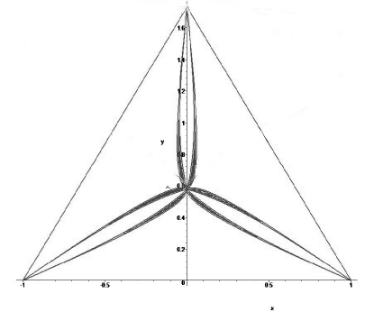
Figure 10: Region  defining the  acute triangle.

Taking into account symmetries, the two inequalities in (6) define the region depicted in Figure 10. We are going to concentrate only on one sixth of the picture. The conditions $0<u<v<w$ are equivalent to $x>0$, $y>0$, and $y<\frac{\sqrt{3}}{3}(1-x)$.

In order to obtain something that we can integrate we need to parameterize the two resulting curves from (6). The idea is to make the substitution $y=t(1-x)$ which will considerably simplify the equations of the two curves. This is a standard procedure of rationalizing a curve if one knows a point with integer coordinates on it (see [21]). The inequality $w(2u^{2}-v^{2})<uv^{2}$ turns into

$$x(9t^{3}+5t^{2}m+9t-3m)-9t^{3}+9t^{2}m+3t-3m<0$$

or

$$x<f(t):=\frac{9t^{3}-9t^{2}m-3t+3m}{9t^{3}+5t^{2}m+9t-3m}.$$

Let us observe that $t$ is less than $\frac{m}{3}$. One the other hand it is obvious that we need to have $v<u\sqrt{2}$, which boils down to $y>n(1-x)$ where $n:=\frac{m}{2\sqrt{2}+1}$. So, in the above inequality involving $x$, the range of $t$ is $[n,m/3]$. One can check that $f$ is well defined on this interval. In addition, $f(n)=1$ and $f(m/3)=0$. The other inequality in (6) reduces to $x>g(t)$ with $g$ defined as in the statement. We denote by $\mathcal{R}$ the region we are interested in, i.e. the right-hand petal going down in Figure 10. The Jacobian of the transformation $(x,y)\to(x,t)$ is $J=1-x$ and so

$$Area(\mathcal{R})=\underset{\mathcal{R}}{\int\int}dxdy=\int_{n}^{m/3}\int_{g(t)}^{f(t)}(1-x)dxdt=\frac{1}{2}\int_{n}^{m/3}(1-g(t))^{2}-(1-f(t))^{2}dt$$

which implies

$$P=Area(\mathcal{R})/(\frac{m}{6})=m\int_{n}^{m/3}(1-g(t))^{2}-(1-f(t))^{2}dt.$$

4.3 Distances to the sides from the circumcenter.

In this section there will be no need to compute any probabilities. Part of the next theorem appeared as a proposed problem in [10].

Theorem 7.

Consider a triangle $ABC$ and let $O$ be its circumcenter. Denote the distances of $O$ to the sides $\overline{BC}$, $\overline{AC}$, and $\overline{AB}$, by $u$, $v$ and $w$ respectively.

(i) The radius $R$, of the circle circumscribed to the triangle $ABC$, satisfies the equation

$$R^{3}-(u^{2}+v^{2}+w^{2})R-2uvw=0,\ if\ \triangle ABC\ is\ acute;$$ (7)

$$R^{3}-(u^{2}+v^{2}+w^{2})R+2uvw=0,\ if\ \triangle ABC\ is\ obtuse;$$ (8)

and (obviously)

$$R=(u^{2}+v^{2}+w^{2})^{\frac{1}{2}},\ if\ \triangle ABC\ is\ a\ right\ triangle.$$ (9)

(ii) Given three positive real numbers $u$, $v$, and $w$, there exists one and only one acute triangle with the distances of the circumcenter to the sides equal to $u$, $v$ and $w$. The previous statement is true if one changes the adjective acute to obtuse.

(iii) The equation (7) has infinitely many integer solutions $(u,v,w,R)\in\mathbb{N}^{4}$ such that $u$, $v$, and $w$ are all different.

Proof.

(i) Denote by $D$, $E$ and $F$ the projections of $O$ on $\overline{AC}$, $\overline{AB}$, and $\overline{BC}$ respectively (see Figure 12 (a)). One can easily prove the identity

$$\cos A+\cos B+\cos C=1+4\sin\frac{A}{2}\sin\frac{B}{2}\sin\frac{C}{2},$$ (10)

where $A$, $B$ an $C$ are the angles of the triangle. In the triangle $\triangle OBC$, $\overline{OF}$ is clearly the angle bisector of $\angle BOC$. First, we assume that the triangle $ABC$ is acute. Because $A$ is less than $90^{\circ}$, $m(\angle BOF)=\frac{m(arc\ \overset{\frown}{BC})}{2}=A$. Hence $\cos A=\frac{u}{R}$, and similarly $\cos B=\frac{v}{R}$, and $\cos C=\frac{w}{R}$. Substituting into (10) we get

$$u+v+w=R+\sqrt{\frac{2(R-u)(R-v)(R-w)}{R}},$$ (11)

which after elimination of the radical sign gives the equation (7).

(ii) First we want to show the existence and uniqueness of an acute triangle with the required property. Let us denote the quantity $\left(\frac{u^{2}+v^{2}+w^{2}}{3}\right)^{1/2}$ by $\omega$ and observe that the AM-GM Inequality gives

$$\omega^{3}\geq uvw.$$

If we consider the cubic polynomial function

$$f(t)=t^{3}-(u^{2}+v^{2}+w^{2})t-2uvw,\ t\in\mathbb{R}$$

observe that $f^{\prime}$ has as critical points $\pm\omega$. There are clearly at most three real solutions of $f(t)=0$. Since $f(0)=-2uvw<0$ and $f(-\omega)=2(\omega^{3}-uvw)\geq 0$, $f$ must have two real zeros in $(-\infty,0)$ (or possibly one with multiplicity two) and a unique positive zero that we will simply denote by $R$. Because $f(u)=-u(v+w)^{2}<0$ , $f(v)=-v(u+w)^{2}<0$, $f(w)=-w(u+v)^{2}<0$ and $f(2\omega)=2(\omega^{3}-uvw)\geq 0$ we see that

$$R\in(\max\{x,y,z\},2\omega].$$

$\underset{(a)\ \text{Distances to sides from the circumcenter}}{\psfig{height=158.99377pt,width=158.99377pt}}$   $\underset{(b)\ \text{Orthocenter's distances to vertices}}{\psfig{height=137.31255pt,width=195.12877pt}}$

Figure 11: Identical problems

The radius $R$ determines the sides $a$, $b$ and $c$ by the formulas $a=2R\sin A=2\sqrt{R^{2}-u^{2}}$, $b=2\sqrt{R^{2}-v^{2}}$ and $c=2\sqrt{R^{2}-w^{2}}$. Without loss of generality we may assume that $w\leq v\leq u$. In order to have a triangle with side lengths $a$, $b$ and $c$ it is necessary and sufficient to have

$$\sqrt{R^{2}-u^{2}}+\sqrt{R^{2}-v^{2}}>\sqrt{R^{2}-w^{2}}$$

or

$$2\sqrt{(R^{2}-u^{2})(R^{2}-v^{2})}>u^{2}+v^{2}-w^{2}-R^{2}.$$

This is trivially verified if we show that $R>(u^{2}+v^{2}-w^{2})^{1/2}$. Since $f((u^{2}+v^{2}-w^{2})^{1/2})=-2w^{2}(u^{2}+v^{2}-w^{2})^{1/2}-2uvw<0$ then we must have $R>(u^{2}+v^{2}-w^{2})^{1/2}$. Once we have the triangle constructed with side lengths $a$, $b$ and $c$, we must check to see if the triangle is acute, i.e. $a^{2}+b^{2}>c^{2}$, $b^{2}+c^{2}>a^{2}$ and $a^{2}+c^{2}>b^{2}$. These inequalities are equivalent to $R>(u^{2}+v^{2}-w^{2})^{1/2}$, $R>(u^{2}-v^{2}+w^{2})^{1/2}$ and $R>(-u^{2}+v^{2}+w^{2})^{1/2}$ respectively, which were shown to be true earlier. We denote the angles of the triangle with sides $a$, $b$, and $c$ by $A^{\prime}$, $B^{\prime}$ and $C^{\prime}$. If we calculate the cosine function for $A^{\prime}$ we get

$$\cos A^{\prime}=\frac{b^{2}+c^{2}-a^{2}}{2bc}=\frac{R^{2}+u^{2}-v^{2}-w^{2}}{2\sqrt{(R^{2}-v^{2})(R^{2}-w^{2})}}.$$

Using (7), which $R$ satisfies, one can show that $\cos A^{\prime}=\frac{u}{R}$. So, $\sin A^{\prime}=\frac{a}{2R}$ which implies that $R$ is the radius of the circle circumscribed about the constructed triangle. Then the distances to the sides from the center of the circumscribed circle must be $u$, $v$ and $w$. Therefore, we have only one triangle that satisfies the required conditions.

For the second part of the claim in (ii) one needs to repeat the above arguments with the appropriate changes. In this case the radius $R$ must satisfy the equation

$$R^{3}-(u^{2}+v^{2}+w^{2})R+2uvw=0.$$ (12)

(iii) One such solution is $u=2$, $v=7$, $w=11$ and $R=14$. This example suggests that one can take $R=uv$ and hope to obtain more solutions of this type. In this case, (7) reduces to

$$(u^{2}-1)(v^{2}-1)=(w+1)^{2}.$$

This equation is satisfied if $v^{2}-1=k^{2}(u^{2}-1)$ for some $k\in\mathbb{N}$, and $zw=k(u^{2}-1)-1$. If we fix $u=2$ for instance, we get Pell’s diophantine equation, $v^{2}-3k^{2}=1$, which is known to have infinitely many integer solutions. The values $u$, $v$ and $w$ are clearly distinct if $k>1$.

There are many different patterns of solutions. Some examples are included in the table below:

u	1	2	2	3	4	4	6	7	8	11	11	12
v	13	7	9	14	14	18	11	19	17	17	19	22
w	22	11	12	25	22	24	14	25	22	21	26	28
R	26	14	16	30	28	32	21	35	32	33	38	42

∎

Let us observe that this discussion of this subsection also solves the problem for $\alpha=HA$, $\beta=HB$ and $\gamma=HC$, where $H$ is the orthocenter of a triangle, i.e. the intersection of its altitudes (see Figure 12(b)). Indeed, one can show that there are very similar formulas for these distances in terms of the sides and angles of the triangle: $HA=2R\cos A$, $HB=2R\cos B$ and $HC=2R\cos C$. Similarly, the problem $\alpha=HD$, $\beta=HE$ and $\gamma=HF$ (Figure 9(a)) leads to the same analysis since $HD=2R\cos A\cos C$.

$\underset{(a)\ \text{Distances to sides from the circumcenter}}{\psfig{height=158.99377pt,width=158.99377pt}}$$\underset{(b)\ \text{The incircle}}{\psfig{height=166.2212pt,width=166.2212pt}}$

Figure 12: Special Cases

4.4 Distances from the center of the incircle to the vertices

First we will show a relation between the radius of the incircle and the distances from the center of the incircle to the vertices. If $I$ is the center of the incircle of the triangle $ABC$, $r$ is the radius of the incircle and we denote $AI$, $BI$ and $CI$ by $u$, $v$ and $w$ respectively as in Figure 12(b), then

$$\sin\frac{A}{2}=\frac{r}{u},\quad\sin\frac{B}{2}=\frac{r}{v},\quad\textup{and}\quad\sin\frac{C}{2}=\frac{r}{w}.$$

From here we infer that

$$\cos\frac{B}{2}=\sqrt{1-\frac{r^{2}}{v^{2}}}\quad\textup{and}\quad\cos\frac{C}{2}=\sqrt{1-\frac{r^{2}}{w^{2}}}.$$

On the other hand, since

$$\sin\frac{A}{2}=\sin\frac{\pi-(B+C)}{2}=\cos\frac{B+C}{2}=\cos\frac{B}{2}\cos\frac{C}{2}-\sin\frac{B}{2}\sin\frac{C}{2}$$

we get the third degree equation in $r$ (with $u$, $v$ and $w$ as parameters)

$$\frac{r}{u}=\sqrt{1-\frac{r^{2}}{v^{2}}}\sqrt{1-\frac{r^{2}}{w^{2}}}-\frac{r^{2}}{vw}\iff\frac{r}{u}+\frac{r^{2}}{vw}=\sqrt{1-\frac{r^{2}}{v^{2}}}\sqrt{1-\frac{r^{2}}{w^{2}}}$$

$$\iff\frac{r^{2}}{u^{2}}+\frac{r^{4}}{v^{2}w^{2}}+2\frac{r^{3}}{uvw}=1-\frac{r^{2}}{v^{2}}-\frac{r^{2}}{w^{2}}+\frac{r^{4}}{v^{2}w^{2}}\iff$$

$$\frac{2}{uvw}r^{3}+\left(\frac{1}{u^{2}}+\frac{1}{v^{2}}+\frac{1}{w^{2}}\right)r^{2}-1=0.$$ (13)

It is easy to see that equation (13) has a unique positive solution which is less than either of the values $u$, $v$, or $w$.

Once we have $r$, a simple geometrical construction shows that $a$, $b$ and $c$ are uniquely determined by $u$, $v$ and $w$. We want to show some relations between the sides of the triangle, the radius of the incircle, and the distances from the center of the incircle to the vertices that will make this clear. Let $P,Q,R$ be the points of intersection of the perpendiculars from $I$ on $BC$, $CA$ and $AB$ respectively. It is well known that

$$PC=QC=\frac{a+b-c}{2};\ QA=RA=\frac{b+c-a}{2},\ \text{and}\ RB=PB=\frac{a+c-b}{2}.$$

Then

$$a+b-c=2\sqrt{w^{2}-r^{2}},\ b+c-a=2\sqrt{u^{2}-r^{2}},\ \textup{and}\ a+c-b=2\sqrt{v^{2}-r^{2}},$$

which leads to

$$\begin{cases}a=\sqrt{v^{2}-r^{2}}+\sqrt{w^{2}-r^{2}},\\ \\ b=\sqrt{u^{2}-r^{2}}+\sqrt{w^{2}-r^{2}},\ \text{and}\ \\ \\ c=\sqrt{u^{2}-r^{2}}+\sqrt{v^{2}-r^{2}}.\end{cases}$$ (14)

Now we will work our way backwards.

Theorem 8.

If $u$, $v$, and $w$ are positive quantities then there is a unique triangle such that the distances from the vertices to the center of the incircle are equal to $u$, $v$, and $w$ respectively.

Proof.

The part about uniqueness follows from the analysis above the statement of the theorem. For existence, we let $r$ be the unique positive solution of (13) and $a$, $b$ and $c$ as given by (14). Then, using Heron’s formula, the area of the triangle is given by

$$A=\sqrt{\sqrt{u^{2}-r^{2}}\sqrt{v^{2}-r^{2}}\sqrt{w^{2}-r^{2}}(\sqrt{u^{2}-r^{2}}+\sqrt{v^{2}-r^{2}}+\sqrt{w^{2}-r^{2}})}$$

and hence the radius of the circle inscribed in the triangle with sides $a$, $b$ and $c$ is

$$r^{\prime}=\frac{2A}{a+b+c}=\sqrt{\frac{\sqrt{u^{2}-r^{2}}\sqrt{v^{2}-r^{2}}\sqrt{w^{2}-r^{2}}}{\sqrt{u^{2}-r^{2}}+\sqrt{v^{2}-r^{2}}+\sqrt{w^{2}-r^{2}}}}.$$

With the analysis we did earlier, we see that if $r^{\prime}=r$, the Pythagorean theorem and formulas (14) will give $AI=u$, $BI=v$ and $CI=w$. So, to complete the proof we need to show that $r=r^{\prime}$. In other words, we must show is that (13) implies

$$r=\sqrt{\frac{\sqrt{u^{2}-r^{2}}\sqrt{v^{2}-r^{2}}\sqrt{w^{2}-r^{2}}}{\sqrt{u^{2}-r^{2}}+\sqrt{v^{2}-r^{2}}+\sqrt{w^{2}-r^{2}}}}.$$

Because $r$ is less than each of $u$, $v$ and $w$, the substitutions

$$m=\frac{u}{r}>1,\quad n=\frac{v}{r}>1,\quad\text{and}\ \ p=\frac{w}{r}>1,$$

make the last equality equivalent to

$$\sqrt{m^{2}-1}+\sqrt{n^{2}-1}+\sqrt{p^{2}-1}=\sqrt{m^{2}-1}\sqrt{n^{2}-1}\sqrt{p^{2}-1}.$$ (15)

We note that, with these substitutions, (13) becomes

$$2mnp+m^{2}n^{2}+n^{2}p^{2}+m^{2}p^{2}-m^{2}n^{2}p^{2}=0.$$ (16)

Eliminating the square roots in a careful way, (15) becomes

$$\sqrt{m^{2}-1}+\sqrt{n^{2}-1}=(\sqrt{m^{2}-1}\sqrt{n^{2}-1}-1)\sqrt{p^{2}-1}$$

$$\iff m^{2}-1+n^{2}-1+2\sqrt{m^{2}-1}\sqrt{n^{2}-1}=(m^{2}-1)(n^{2}-1)(p^{2}-1)+p^{2}-1$$

$$-2(p^{2}-1)\sqrt{m^{2}-1}\sqrt{n^{2}-1}.$$

Using (16) this last equality simplifies to $p\sqrt{m^{2}-1}\sqrt{n^{2}-1}=mn+p$ which, after getting rid of the square roots, becomes (16). ∎

Corollary 4.

Given $u$, $v$ and $w$ three positive real numbers, the triangle ensured by Theorem 8 is acute if and only if

$$\begin{cases}\sqrt{2}u^{2}vw+u^{2}(v^{2}+w^{2})-v^{2}w^{2}>0,\\ \\ \sqrt{2}uv^{2}w+v^{2}(u^{2}+w^{2})-u^{2}w^{2}>0,\ and\\ \\ \sqrt{2}uvw^{2}+w^{2}(u^{2}+v^{2})-u^{2}v^{2}>0.\end{cases}$$ (17)

In the context of the broken stick problem, if $u=\alpha$, $v=\beta$ and $w=\gamma$, the probability that the triangle given by Theorem 8 is acute is approximately $0.1962$.

Proof.

The triangle is acute if and only if

$$\sin\frac{A}{2}<\frac{1}{\sqrt{2}},\ \sin\frac{B}{2}<\frac{1}{\sqrt{2}},\quad\textup{and}\quad\sin\frac{C}{2}<\frac{1}{\sqrt{2}}.$$

This means that

$$\frac{r}{u}<\frac{1}{\sqrt{2}},\ \frac{r}{v}<\frac{1}{\sqrt{2}},\quad\textup{and}\quad\frac{r}{w}<\frac{1}{\sqrt{2}}\iff r<\min\left\{\frac{u}{\sqrt{2}},\frac{v}{\sqrt{2}},\frac{w}{\sqrt{2}}\right\}.$$

Since $r$ is the unique positive solution of (13) and the derivative of the function $g(t)=\frac{2t^{3}}{uvw}+(1/u^{2}+1/v^{2}+1/w^{2})t^{2}-1$ is positive for $t>0$, this is equivalent to $g(\frac{u}{\sqrt{2}})>0$, $g(\frac{v}{\sqrt{2}})>0$, and $g(\frac{w}{\sqrt{2}})>0$. This translates into (17). The equations that define the probability are of degree four and we could only find the probability experimentally. $\hfill\blacksquare$

The ratio $P(obtuse)/P(acute)\approx 4.1$ balances out the previous cases.

5 Further problems and a summary

One may investigate using this technique the case in which $\alpha$, $\beta$ and $\gamma$ are the symmedians of a triangle. The formula for the symmedian corresponding to vertex $A$ is given by $sm_{a}=\frac{bc}{b^{2}+c^{2}}\sqrt{2(b^{2}+c^{2})-a^{2}}$. This formula is very similar to the angle bisector formula but the situation seems to be very different of the one discussed in Section 4.1. We have no answer to this problem.

There are certainly interesting generalizations that can be considered and in some directions they have already appeared in the literature. For instance, Carlos D’Andrea and Emiliano Gomez ([2]) showed that if $n-1$ ($n\geq 3$) breaking points are considered, the probability of having an $n$-gon with the resulting segments is equal to $\displaystyle 1-n/2^{n-1}$. This result also appeared in [3], where the solution is derived by solving another geometric probability question, called by the authors, The Semicircle Problem ([19]). In fact, it was shown to be equivalent to this problem: “If $n+1$ points are randomly selected on the circumference of a circle, what is the probability that they will all fall within some semicircle?” Another direction of further investigations along these lines is to go into space, so to speak, and ask: “If the stick breaks into six segments, what is the probability that the segments are the sides of a tetrahedron?”

Let us briefly discuss the following generalization which appeared in [23] as a proposed problem. It is worth mentioning that the solution to this problem was from its author, Professor Gheorghe Mihoc, and it was based on a different idea than the one we have included below.

Proposition 1.

Given an arbitrary triangle with sides $a$, $b$ and $c$, the probability that the distances from a point inside the triangle to the sides of the triangle form a triangle, is equal to

$$\frac{2abc}{(a+b)(b+c)(c+a)}.$$

$$\underset{Figure\ 9:\ \text{$DEF$ triangle}}{\psfig{height=115.63243pt,width=158.99377pt}}$$

For the sake of completeness we sketch a proof of this proposition. We refer to Figure 9. Triangle $DEF$ is given by the points where the angle bisectors intersect the sides of triangle $ABC$. First, one shows that the region determined by the interior of triangle $DEF$ is the region that gives the desired probability. Using the Angle Bisector Theorem one can show that

$$\frac{Area(\triangle BDF)}{Area(\triangle ABC)}=\frac{ac}{(b+c)(a+b)},$$

and also the other two equalities obtained by cyclic permutation of the sides $a$, $b$ and $c$. The formula given, now follows from an algebraic identity

$$(a+b)(b+c)(c+a)-[(a+b)ab+(b+c)bc+(c+a)ca]=2abc.$$

We observe that this probability has its greatest value of $1/4$ when $a=b=c$. This means, the probability is at a maximum when $ABC$ is equilateral.

Another question one may ask is: “how does the answer in Theorem 1 change if $\alpha$, $\beta$ and $\gamma$ are computed relative to an arbitrary triangle as in Proposition 1?” A general answer is probably quite complicated because the curve $\alpha^{2}=\beta^{2}+\gamma^{2}$ may be an arc of an ellipse or an arc of a hyperbola. For example, if $a=b=\frac{15}{4}$ and $c=6$, one of the conics at the boundary of the region defining the probability is an ellipse and the other two are hyperbolas. The probability in Theorem 1 becomes

$$P=\frac{25}{28}+\frac{25}{32}\ln\frac{13}{5}-\frac{100}{49}\sqrt{14}\arcsin\left(\frac{\sqrt{7}}{13}\right).$$

Finally, let us summarize our results:

Case Probability Acute Ratio $\frac{Obtuse}{Acute}$ classical case $\frac{1}{4}$ $\ln(\frac{8}{e^{2}})$ 2.146968 medians $\frac{1}{4}$ $\frac{1}{3}-\frac{5}{9}\ln\left(\frac{8}{5}\right)$ 2.461635121 altitudes $\frac{4}{25}\left(3\sqrt{5}\ln\frac{3+\sqrt{5}}{2}-5\right)$ 0.07744388 2.008 r,s,t $\frac{5}{27}$ 0.047 2.87 angle bisector 1 0.1195 7.36 $IA$, $IB$, $IC$ 1 0.1962 4.1 excircles radii 1 $\frac{24\sqrt{7}}{49}\arcsin(\frac{\sqrt{14}}{8})-\frac{2}{7}$ 1.9 $h_{a}$, $w_{a}$ and $m_{a}$ 1 0.042234 22.7

Acknowledgements. We thank Professor Albert VanCleave who helped us significantly improve the exposition of this article. We also want to thank Professors Charles M. Grinstead and J. Laurie Snell for writing the book [8] and providing that in pdf format. The first author learned about The Broken Stick Problem from their book (Problem 12, page 73) while teaching the Introduction to Probability course at CSU in the Spring of 2008.

Eugen J. Ionascu Department of Mathematics, Columbus State University, Columbus, GA 31907, US, e-mail: math@ejionascu.ro

Gabriel Prajitura The College at Brockport, State University of New York, US e-mail: gprajitu@brockport.edu

References

- [1] B. Eisenberg and R. Sullivan, Random triangles in dimensions, Amer. Math. Monthly, 103(1996), no. 4, 308–318.
- [2] C. D’Andrea and E. Gomez, The broken spaghetti noodle, Amer. Math. Monthly, 113 (2006), 555–557.
- [3] T. J. Bannon and R. E. Bradley, Mind the gap, College Math. J., 39(2008), 95–99.
- [4] M. Gardner, The Second Scientific American Book of Mathematical Puzzles and Diversions, University of Chicago Press, Chicago, 1987.
- [5] G. S. Goodman, The problem of the broken stick reconsidered, Math. Intelligencer, 30 (2008), 43–49.
- [6] R. K. Guy, There are three times as many obtuse-angled triangles as there are acute-angled ones, Math. Mag., 66(1993), 175–179.
- [7] L. A. Graham, Ingenious Mathematical Problems and Methods, Dover Publications, Inc., New York, 1959.
- [8] C. M. Grinstead and J. L. Snell, Introduction to Probability, American Mathematical Society, 1997.
- [9] R. Honsberger, Ingenuity in mathematics, Mathematical Association of America, Washington, D.C., 1970.
- [10] E. J. Ionascu, Problem 11443, Amer. Math. Monthly, 116 (2009), 548.
- [11] E. J. Ionascu, Problem 11663, Amer. Math. Monthly, 119 (2012), 699.
- [12] D. Ippolito, The spaghetti problem problem, Mathematics Teacher, 93 (2000), 422–426.
- [13] Y. Isokawa, Geometric probabilities concerninig large random triangles in the hyperbolic plane, Kodai Math. J., 23 (2000), 171–186.
- [14] A. Johnson, Geometric Probability, COMAP Inc. (1995), 47–48.
- [15] K. Kawasaki, Proofs without words, Math. Mag., Vol. 78(2005), 213.
- [16] C. L. Lee and K. B. Wong, A note on the broken stick problem, Menemui Matematik (Discovering Mathematics), 25(2003), 20–24.
- [17] R. Mironescu and L. Panaitopol, The existence of triangles with prescribed angle bisector lengths, Amer. Math. Monthly, 101 (1994), 58–60.
- [18] H. , Calcul des Probabilits, George Carte, Paris, 1896; 2nd ed., Gauthier-Villars, 1912; repr. Jacques Gabay, Paris, 1981.
- [19] A. Mood, F. Graybill, and D. Boes, Introduction to the Theory of Statistics, 3rd ed., McGraw-Hill, 1974.
- [20] H. Samelson, Proof without words, Math. Mag., 76(2003), 225.
- [21] I. Shafarevich, Basic Algebraic Geometry, Springer-Verlag, Second Edition, Vol I, 1994.
- [22] The moderators and examiners, Solutions to problems and riders proposed in the Senate House examination for 1854, MacMillan, Cambridge, 1854.
- [23] V. Gh. Voda, Triunghiul-Ringul (The triangle-the boxing ring-in Romanian) Albatros Publishing, Bucharest, 1979.
- [24] D. Wells, Problem 1232, Pi Mu Epsilon, (2010), 560.