Effective Pedestrian Detection Using Center-symmetric Local Binary/Trinary Patterns

Abstract

Accurately detecting pedestrians in images plays a critically important role in many computer vision applications. Extraction of effective features is the key to this task. Promising features should be discriminative, robust to various variations and easy to compute. In this work, we present novel features, termed dense center-symmetric local binary patterns (CS-LBP) and pyramid center-symmetric local binary$/$ternary patterns (CS-LBP$/$LTP), for pedestrian detection. The standard LBP proposed by Ojala et al. [1] mainly captures the texture information. The proposed CS-LBP feature, in contrast, captures the gradient information and some texture information. Moreover, the proposed dense CS-LBP and the pyramid CS-LBP$/$LTP are easy to implement and computationally efficient, which is desirable for real-time applications. Experiments on the INRIA pedestrian dataset show that the dense CS-LBP feature with linear supporct vector machines (SVMs) is comparable with the histograms of oriented gradients (HOG) feature with linear SVMs, and the pyramid CS-LBP$/$LTP features outperform both HOG features with linear SVMs and the start-of-the-art pyramid HOG (PHOG) feature with the histogram intersection kernel SVMs. We also demonstrate that the combination of our pyramid CS-LBP feature and the PHOG feature could significantly improve the detection performance—producing state-of-the-art accuracy on the INRIA pedestrian dataset.

I Introduction

The ability to detect pedestrians in images has a major impact on applications such as video surveillance [2], smart vehicles [3, 4], robotics [5]. Changing variations in human body poses and clothing, combined with varying cluttered backgrounds and environmental conditions, make this problem far from being solved. Recently, there has been a surge of interest in pedestrian detection  [6, 7, 8, 9, 10, 11, 12, 13, 14, 15, 16, 17, 18, 19]. One of the leading approaches for this problem is based on sequentially applying a classifier at all the possible subwindows, which are obtained by exhaustively scanning the input image in different scales and positions. For each sliding window, certain feature sets are extracted and fed to the classifier, which is trained beforehand using a set of labeled training data of the same type of features. The classifier then determines whether the sliding window contains a pedestrian or not.

Driven by the development of object detection and classification, promising performance on pedestrian detection have been achieved by:

1. using discriminative and robust image features, such as Haar wavelets [6], region covariance [10, 12], HOG [8, 9] and PHOG [20];

2. using a combination of multiple complementary features [14, 21];

3. including spatial information [20];

4. the choices of classifiers, such as support vector machines (SVMs) [8, 20], boosting [22, 23].

Feature extraction is of the center importance here. Features must be robust, discriminative, compact and efficient. To date, HOG is still considered as one of the state-of-the-art and most popular features used for pedestrian detection [8]. One of its drawbacks is the heavy computation. Maji et al. [20] introduced the PHOG feature into pedestrian detection, and their experiments showed that PHOG can yield better classification accuracy than the conventional HOG and is much computationally simpler and have smaller dimensions. However, these HOG-like features, which capture the edge or the local shape information, could perform poorly when the background is cluttered with noisy edges [14].

Our goal here is to develop a feature extraction method for pedestrian detection that, in comparison to the state-of-the-art, is comparable in performance but faster to compute. A conjecture is that, if both the shape and texture information are used as the features for pedestrian detection, the detection accuracy is likely to increase. The center-symmetric local binary patterns feature (CS-LBP) [24], which is a modified version of the LBP texture feature [25], inherits the desirable properties of both texture features and gradient based features. In addition, they are computationally cheaper and easier to implement. Furthermore, CS-LBP can be extended to center-symmetric Local Trinary Patterns (CS-LTP), which is more descriptive and less sensitive to noise in uniform image regions. In this work, we introduce the CS-LBP$/$LTP features into pedestrian detection:

1. We propose the dense CS-LBP feature, in the approach similarity as the HOG feature [8], which was carefully developed to work well with linear SVMs for pedestrian detection.

2. We propose the pyramid CS-LBP$/$LTP features, in the approach similarity as the PHOG feature [20], which is muti-scale feature and producing the state-of-the-art accuracy with HIKSVMs on the INRIA pedestrian dataset.

Experiments on the INRIA pedestrian dataset show that the dense CS-LBP feature with linear SVMs performs as well as the HOG feature with linear SVMs, and the pyramid CS-LBP feature with HIKSVMs [20] outperforms the state-of-the-art PHOG features with HIKSVMs. The pyramid CS-LTP feature can achieve even better performances.

The key contributions of this work can be summarized as follows.

1. To our knowledge, it is the first time to apply the CS-LBP feature to pedestrian detection. The standard LBP feature captures the detailed texture information, which is usually harmful for pedestrian detection, e.g., the rich textures on the cloth of a pedestrian. Besides, the bin number of the standard LBP operator is 256, which leads a huge dimensional descriptor of a detection window. On the contrary, the CS-LBP feature captures the shape information and some salient texture information, which is very useful for pedestrian detection. The bin number of the CS-LBP is 16, which is much smaller than the standard LBP.

2. We propose the CS-LTP feature, which is even more distinctive than the CS-LBP feature, for the first time.

3. We apply the pyramid structure, which can can capture richer spatial information, to CS-LBP and CS-LTP for the first time.

4. We show that the detection performance can be further improved significantly by combining our proposed pyramid CS-LBP$/$LTP features with the PHOG feature.

The rest of the paper is organized as follows. In Section II, we briefly describe the LBP operator, the LTP operator, and the CS-LBP operator. In Section III, we give the details of the dense CS-LBP pedestrian detection approach. In Section IV, we propose the pyramid CS-LBP$/$LTP features based pedestrian detection approach. The results of numerous experiments and some study on feature combination are presented in Section V. Section VI concludes the paper.

II Preliminaries

II-A The LBP and LTP features

LBP is a texture descriptor that codifies local primitives (such as curved edges, spots, flat areas) into a feature histogram. LBP and its extensions outperform existing texture descriptors both with respect to performance and to computational efficiency [1].

The standard version of the LBP feature of a pixel is formed by thresholding the 3$\times$3-neighborhood of each pixel with the center pixel’s value . Let $g_{c}$ be the center pixel graylevel and $g_{i}\,(i=0,1,\cdots,7)$ be the graylevel of each surrounding pixel. If $g_{i}$ is smaller than $g_{c}$, the binary result of the pixel is set to 0, otherwise to 1. All the results are combined to a 8-bit binary value. The decimal value of the binary is the LBP feature. See Fig. 1 for an illustration of computing the basic LBP feature.

Figure 1: Illustration of the basic LBP operator.

In order to be able to cope with textures at different scales, the original LBP has been extended to arbitrary circular neighborhoods [25] by defining the neighborhood as a set of sampling points evenly spaced on a circle centered at a pixel to be labeled. It allows any radius and number of sampling points. Bilinear interpolation is used when a sampling point does not fall in the center of a pixel. Let LBP_p,r denote the LBP feature of a pixel’s circular neighborhoods, where $r$ is the radius of the circle and $p$ is the number of sampling points on the circle. The LBP_p,r can be computed as follows:

$${\rm LBP}_{p,r}=\sum_{i=0}^{p-1}S(g_{i}-g_{c})2^{i},\,S(x)=\begin{cases}1&\text{if $x\geq 0$,}\\ 0&\text{ otherwise.}\end{cases}$$ (1)

Here $g_{c}$ is the center pixel’s graylevel and $g_{i}\,(i=0,1,\cdots,7)$ is the graylevel of each sampling pixel on the circle. See Fig. 2 for an illustration of computing the LBP feature of a pixel’s circular neighborhoods with $r=1$ and $p=8$.

Figure 2: The LBP operator of a pixel’s circular neighborhoods with $r=1$, $p=8$.

Ojala et al. [25] proposed the concept of “uniform patterns” to reduce the number of possible LBP patterns while keeping its discrimination power. An LBP pattern is called uniform if the binary pattern contains at most two bitwise transitions from $0$ to $1$ or vice versa when the bit pattern is considered circular. For example, the bit pattern $11111111$ (no transition), $00001100$ (two transitions) are uniform whereas the pattern $01010000$ (four transitions) is not. The uniform pattern constraint reduces the number of LBP patterns from $256$ to $58$ and is successfully applied to face detection in [26].

In order to make LBP less sensitive to noise, particularly in near-uniform image regions, Tan and Triggs [27] extended LBP to 3-valued codes, called local trinary patterns (LTP). If each surrounding graylevel $g_{i}$ is in a zone of width $\pm t$ around the center graylevel $g_{c}$, the result value is quantized to 0. The value is quantized to $+1$ if $g_{i}$ is above this and is quantized to $-1$ if $g_{i}$ is below this. The LTP_p,r can be computed as:

$${\rm LTP}_{p,r}=\sum_{i=0}^{p-1}S(g_{i}-g_{c})3^{i},\,S(x)=\begin{cases}1&\text{if $x\geq t$,}\\ 0&\text{if $|x|<t$,}\\ -1&\text{if $x\leq t$,}\end{cases}$$ (2)

Here $t$ is a user-specified threshold. Fig. 3 shows the encoding procedure of LTP. For simplicity, Tan and Triggs [27] used a coding scheme that splits each ternary pattern into its positive and negative halves as illustrated in Fig. 4, treating these as two separate channels of LBP codings for which separate histograms are computed, combining the results only at the end of the computation.

Figure 3: Illumination of the basic LTP operator.

Figure 4: Splitting the LTP code into positive and negative LBP codes.

II-B The CS-LBP/LTP patterns

The CS-LBP is another modified version of LBP. It is originally proposed to alleviate some drawbacks of the standard LBP. For example, the original LBP histogram could be very long and the original LBP feature is not robust on flat images. As demonstrated in Fig. 5, instead of comparing the graylevel of each pixel with the center pixel, the center-symmetric pairs of pixels are compared. The CS-LBP features can be computed by:

$$\textrm{CS-LBP}_{p,r,t} =\sum_{i=0}^{N/2-1}S(|g_{i}-g_{i+(N/2)}|)2^{i},$$ (3)

$$S(x) =\begin{cases}1&\text{if $x\geq t$,}\\ 0&\text{ otherwise.}\end{cases}$$ (4)

Here $g_{i}$ and $g_{i+N/2}$ correspond to the graylevel of center-symmetric pairs of pixels ($N$ in total) equally spaced on a circle of radius $r$. Moreover, $t$ is a small value used to threshold the graylevel difference so as to increase the robustness of the CS-LBP feature on flat image regions. From the computation of CS-LBP, we can see that the CS-LBP is closely related to the gradient operator, because like some gradient operators, it considers graylevel differences between pairs of opposite pixels in a neighborhood. In this way the CS-LBP feature takes advantage of the properties of both the LBP and gradient based features. Fig. 6 shows images of LBP, orientation bin and CS-LBP. The LBP image is obtained by replacing the graylevel of each pixel of the original image with the pixel’s LBP value; the orientation bin image is obtained by replacing the graylevel of each pixel with its orientation bin number (the 16 orientation bins are evenly spaced over $0^{\circ}-360^{\circ}$); the CS-LBP image is obtained by replacing the graylevel of each pixel of the original image with the pixel’s CS-LBP value. We can see that the CS-LBP captures the edges and the salient textures. In [24], the authors used the CS-LBP descriptor to describe the region around an interest point and their experiments show that the performance is almost equally promising as the popular SIFT descriptor [28]. The authors also compared the computational complexity of the CS-LBP descriptor with the SIFT descriptor and it has been shown that the CS-LBP descriptor is on average $2$ to $3$ times faster than the SIFT. That is because the CS-LBP feature needs only simple arithmetic operations while the SIFT requires time consuming inverse tangent computation when computing the gradient orientation.

Figure 5: The CS-LBP features for a neighborhood of $8$ pixels.

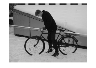
(a) Original image.

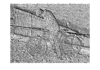
(b) LBP image.

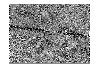
(c) Orientation bin image.

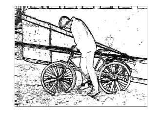
(d) CS-LBP image.

Figure 6: Example images of LBP, orientation bin and CS-LBP. (a) The original image selected from INRIA dataset. (b) The LBP image, which is obtained by replacing the graylevel of each pixel of the original image with the pixel’s LBP value. (c) The orientation bin image, which is obtained by replacing the graylevel of each pixel of the original image by the pixel’s orientation bin number. (d) The CS-LBP image, which is obtained by replacing the graylevel of each pixel of the original image by the pixel’s CS-LBP value.

Similarly as “uniform LBP patterns”, we propose “uniform CS-LBP patterns” to reduce the original CS-LBP pattern numbers. The possibility of each CS-LBP pattern is not equally distributed. The 8 patterns with bigger possibilities are called uniform while the rests are called non-uniform. We computed the CS-LBP patterns of 741 images in the INRIA dataset (288 images containing pedestrians and 453 images without pedestrians) with $t=0.022$ and found that 87.39% of the patterns are uniform, shown in Table I.

The CS-LTP patterns and the uniform CS-LTP patterns can be developed similarity as the CS-LBP and the uniform CS-LBP.

TABLE I: The distribution of the CS-LBP patterns (uniform and non-uniform) with $t=0.022$ on the INRIA pedestrian dataset.

Uniform pattern	0000	0001	0011	0100	0111	1000	1101	1111	Total
Percent. (%)	7.67	7.34	2.19	5.65	3.47	2.28	3.52	55.26	87.39
Non-uniform pattern	0010	0101	0110	1001	1010	1011	1100	1110	Total
Percent. (%)	2.16	1.09	1.84	2.18	0.52	1.51	1.85	1.45	12.61

III Pedestrian detection using dense CS-LBP feature

III-A The approach

In this section, we introduce the implementation details of our dense CS-LBP feature based pedestrian detection approach. Detailed comparisons between different parameter choices are carried out later. The key steps are as follows.

1. We normalize the graylevel of the input image to reduce the illumination variance in different images. After the graylevel normalization is performed, all input images have graylevel ranging from 0 to 1.

2. Each detection window is split into equally sized cells and the cells are grouped into bigger blocks. The size of our detection window is $64\times 128$ and the size of each block is $32\times 32$ and each block contains $2\times 2$ cells of $16\times 16$ pixels, as shown in Fig. 7. As in [8], there are overlaps among adjacent blocks (overlapping $1/2$ block).

3. The 3D histogram of each block is computed similarly as the SIFT descriptor: The gradient magnitude and the CS-LBP value at each pixel in every cell are computed, as the arrows shown on the left of Fig. 7. These are weighted by a Gaussian window centered in the middle of the block with $\sigma=0.5\times\rm blockwidth$, indicated by overlaid circle. The weighted values of all the points in a cell are accumulated into histograms by summarizing the contents over the cell. On the right of Fig. 7, it shows 16 bins for the histogram of each cell, with the length of each arrow corresponding to the magnitude of the histogram entry. A 3D histogram of the cells’ locations ($x$ and $y$ shown on the right of Fig. 7) and the cells’ CS-LBP values is proposed for the block. In order to avoid boundary effects in which the 3D histogram abruptly changes as a feature shifts from one cell to another, bilinear interpolation over horizontal and vertical dimensions is used to share the weights of the features between four nearest cells. Interpolation over CS-LBP value dimension is not carried out because the CS-LBP feature is quantized by its nature [24].

4. The 3D histogram of each block is converted into a vector and is normalized. Let $v$ be the unnormalized descriptor, $\|v\|_{k}$ be its $k$-norm for $k=1,2$, and $\epsilon$ be a small constant. The commonly used normalization schemes are [8]:

   1. $\ell_{1}$-norm, $v\leftarrow v/(\|v\|_{1}+\epsilon)$;

   2. $\ell_{1}$-sqrt, $\ell_{1}$-norm followed by square root $v\leftarrow v/\sqrt{(\|v\|_{1}+\epsilon)}$;

   3. $\ell_{2}$-norm, $v\leftarrow v/\sqrt{(\|v\|^{2}_{2}+\epsilon)}$;

   4. $\ell_{2}$-hys, $\ell_{2}$-norm followed by clipping (limiting the maximum values of $v$ to $0.2$) and re-normalizing.

   In our implementation, $\ell_{1}$-sqrt normalization gives the best result. The difference between these normalization schemes are not significant.

5. The histograms of all the blocks in a detection window are concatenated to form a CS-LBP descriptor. This is used as the input for the linear SVMs classifier.

6. The detection window slides on the input images in all positions and scales, with a fixed scale factor 1.09 and a fixed step size $8\times 8$. The descriptor of each detection window is classified by the pretrained linear SVM classifier. As in [9], non maximal suppression [29] clustering is used to merge the multiple overlapping detections in the 3D position and scale space.

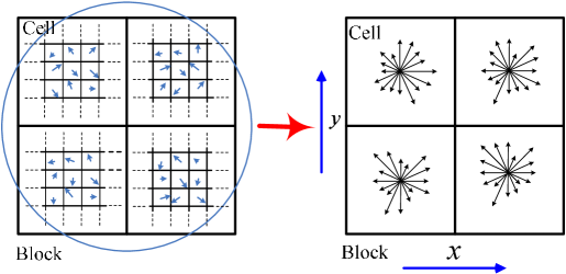
Figure 7: A 3D histogram of each cell’s locations ($x$ and $y$) and the cell’s CS-LBP values (16 bins) is proposed for the block: The gradient magnitude and the CS-LBP value at each pixel in every cell are computed. The magnitudes are weighted by a Gaussian window centered in the middle of the block with $\sigma=0.5\times\rm blockwidth$, indicated by overlaid circle. The weighted values of all the points in a cell are accumulated into histograms by summarizing the contents over the cell. On the right of the figure, it shows 16 bins of each cell’s histogram, with the length of each arrow corresponding to the magnitude of the histogram entry.

III-B Parameters selection

There are various parameter configurations that can be chosen to optimize the performance of the CS-LBP feature based detection approach. These include choosing the block size and cell size, $\sigma$ of the Gaussian weighing window, using interpolate bilinearly over $x$ and $y$ dimensions when building the histogram, the normalization method and the overlapping size of blocks.

We train a linear SVMs classifier using the training set described in Section V-A and use the $1,132$ cropped human samples with size $70\times 134$ (a margin of 3 pixels around each side) from the test dataset as the positive test set. We randomly select $4,530$ patches with size $64\times 128$ from the 453 human free images in the test dataset as negative test set. Then we use the pretrained classifier to classify between the positive samples and the negative samples. The classification rate of the positive samples versus false positive rate is used to evaluate the performances of different parameter selections.

We compare the performances of our CS-LBP features with different block size and cell size configurations in Fig. 8. It shows that 32$\times$32 pixels blocks with 16$\times$16 pixels cells performs better than 16$\times$16 pixels blocks with 8$\times$8 pixels cells.

We explore the effect of the Gaussian weight window in Fig. 8. The results show that a Gaussian weight window with $\sigma=16$ (half block width) can improve the performance significantly. However, if $\sigma$ is too big or small, the performance is almost identical as the case when there is no Gaussian weight.

Fig. 8 shows that using bilinear interpolation when building the histogram of each block can increase the performance.

We also evaluate four different normalization schemes in Fig. 8. The schemes are: $\ell_{2}$-norm, $\ell_{2}$-hys, $\ell_{1}$-norm, $\ell_{1}$-sqrt. Fig. 8 shows that $\ell_{1}$-sqrt performs best and $\ell_{1}$-norm performs very close to $\ell_{1}$-sqrt. $\ell_{2}$-hys and $\ell_{2}$-norm are about $2\%$ worse than $\ell_{1}$-sqrt when false positive rate is $0.03$. The performance of without normalization is worst.

Fig. 8 shows the performance of overlapping blocks. We can see from Fig. 8 that the detection rate increases when overlapping $1/2$ blocks, and overlapping $3/4$ blocks performs equally to overlapping $1/2$. Overlapping $1/2$ is a better choice because its descriptor dimension is much smaller than overlapping $3/4$.

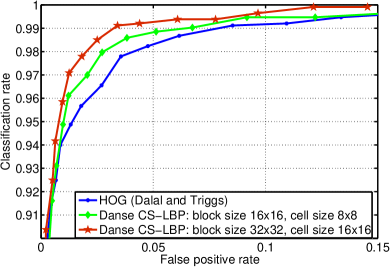
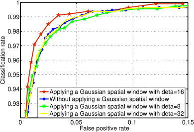
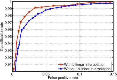
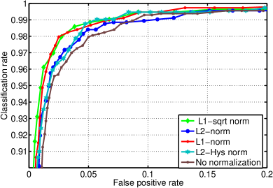
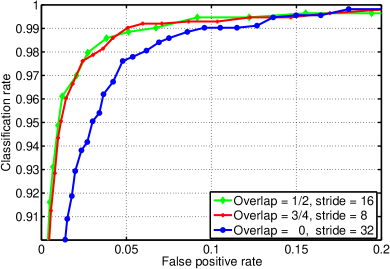
Figure 8: Experimental results. (a) Performance comparison of the CS-LBP feature with different block sizes and cell sizes. (b) Performance comparison of the CS-LBP feature with different Gaussian weight factor $\sigma$. (c) Performance comparison of the CS-LBP feature with and without bilinear interpolation. (d) Performance comparison of the CS-LBP features with different normalization methods. (e) Performance comparison of the CS-LBP features with different rate of overlapping.

In conclusion, the CS-LBP feature based approach has the following descriptions: $64\times 128$ detection windows, $32\times 32$ pixels block of four $16\times 16$ pixels cells; overlapping $1/2$ block (block spacing stride of $16$ pixels); the Gaussian with $\sigma=16$; $\ell_{1}$-sqrt block descriptor normalization; the descriptor length of each detection window is $1334$ ($3\times 7\times 4\times 16$ ); the detection window slides with a fixed step size of 8 pixels and a fixed scale factor of 1.09 in the 3D position and scale space.

IV Pedestrian detection using pyramid CS-LBP/LTP features

Motivated by the image pyramid representation in [30] and the HOG feature [8], Bosch et al. [31] proposed the PHOG descriptor, which consists of a pyramid of histograms of orientation gradients, to represent an image by its local shape and the spatial layout of the shape. Experiments showed that the PHOG feature together with the histogram intersection kernel can bring significant performance to object classification and recognition. Maji et al. [20] introduced the PHOG feature into pedestrian detection and achieved the current state-of-the-art on pedestrian detection. In this section, we propose the pyramid CS-LBP$/$LTP features based pedestrian detection approach.

IV-A The pyramid CS-LBP$/$LTP features

Because the LTP patterns can be divided into two separate channels of LBP patterns, we only illustrate the computation of the pyramid CS-LBP features. Our features of a $64\times 128$ detection window are computed as follows ( Fig. 9 shows the first three steps of computing the features):

1. We compute the CS-LBP value and the gradient magnitude of each pixel of the input grayscale image (detection window). The CS-LBP value is computed as 3 with $t=0.022$. Then we obtain 16 layers of gradient magnitude images corresponding to each CS-LBP pattern. We call them edge energy responses of the input image. Fig. 10 shows the 16 layers of edge energy responses of the example image from INRIA dataset. We can see that the first layer mainly captures the contours, the 16th layer mainly captures the detailed textures or cluttered background, the rests capture spacial edges or textures. The responses in the first layer is much bigger than those in the 16th layer. That is because contours are more important than detailed textures to detect a pedestrian. Sometimes the detailed textures (e.g., textures on the clothes of pedestrians) are harmful to pedestrian detection.

2. Each layer of the response image is $\ell_{1}$ normalized in non overlapping cells of fixed size $y_{n}\times x_{n}$ ($y_{n}=16$, $x_{n}=16$) so that the normalized gradient values in each cell sum to unity.

3. At each level $l\in\{1,2,...L\}$, the response image is divided into non overlapping cells of size $y_{l}\times x_{l}$, and a histogram with 16 bins is constructed by summing up normalized response within the cell. In our case, $L=4$, $y_{1}=x_{1}=64$, $y_{2}=x_{2}=32$, $y_{3}=x_{3}=16$, $y_{4}=x_{4}=8$. So we obtain 2, 8, 32, and 128 histograms at level $l=1$, 2, 3 and 4 respectively.

4. The histograms of each level is normalized to sum to unity. This normalization ensures that the edge or texture rich images are not weighted more strongly than others.

5. The features at a level $l$ are weighted by a factor $w_{l}$ ($w_{1}=1$, $w_{2}=2$, $w_{3}=4$, $w_{4}=9$), and the features at all the levels are concatenated to form a vector of dimension $2,720$, which is called pyramid CS-LBP features.

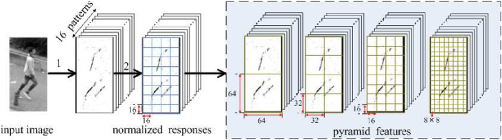
Figure 9: The first three steps of computing the pyramid CS-LBP feature. (1) Edge energy responses corresponding to each CS-LBP pattern of the input image are computed. (2) The responses are $\ell_{1}$ normalized over all layers in each non overlapping $16\times 16$ cells independently so that the normalized gradient values in each cell sum to unity. (3) The features at each level is extracted by concatenating the histograms, which are constructed by summing up the normalized response within each cell at the level. The cell size at level 1, 2, 3 and 4 are $64\times 64$, $32\times 32$, $16\times 16$ and $8\times 8$ respectively.

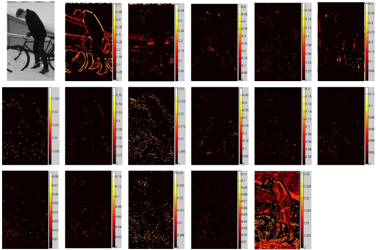
Figure 10: Edge energy responses of an example image. The first image is the input image and the rests are its 16 layers of edge energy responses corresponding to each CS-LBP pattern. In order to show the response images more clearly, the response images are plotted out in color format by indexing the values to hot colormap. On the right of every response iamges shows the corresponding colorbar.

The precess of computing pyramid uniform CS-LBP features is almost same as pyramid CS-LBP. The only difference lies in the first step. In the first step, the edge energy responses corresponding to the 8 different uniform patterns are count into 8 different layers and the edge energy responses corresponding to all the 8 non-uniform patterns are count into one layer. So we obtain 9 layers of edge energy responses of the input image.

IV-B Pedestrian detection based on pyramid CS-LBP$/$LTP features

The first major component of our approach is feature extraction. We perform the graylevel normalization of the input image so that the input image have the graylevel ranged from 0 to 1. Then the detection window slides on the input images in all positions and scales, with a fixed step size $8\times 8$ and a fixed scale factor $1.09$. We follow the steps in Sec. IV-A to compute the pyramid CS-LBP$/$LTP features of each $64\times 128$ detection window.

The second major component of our approach is the classifier. We use IKSVMs [20] as the classifier. The histogram intersection kernel,

$$k_{\rm{HI}}(h_{a},h_{b})=\sum_{i=1}^{n}{\rm{min}}(h_{a}(i),h_{b}(i))$$ (5)

was original proposed by Swain and Ballard [32] for color-based object recognition and has been shown to be a suitable measurement of similarity between histogram $h_{a}$ and $h_{b}$ ( $n$ is the length of the histogram). It is further shown to be positive definite [33] and can be used as a kernel for classification using SVMs. Compared to linear SVMs, histogram intersection kernel involves great computational expense. Maji et al. [20, 34] approximated the histogram intersection kernel for faster execution. Their experiments showed that the approximate IKSVMs consistently outperform linear SVMs at a modest increase in running time.

The third major component of our approach is the merging of the multiple overlapping detections using non maximal suppression [9]. After merging, detections with bounding boxes and confidence scores are obtained.

V Experiments

V-A Experiment setup

Datasets. We perform the experiments on INRIA human dataset [8], which is one of the most popular publicly available datasets. The datasets consist of a training set and a test set. The training set contains $1,208$ images of size $96\times 160$ pixels (a margin of $16$ pixels around each side) of human samples ($2,416$ mirrored samples) and $1,218$ pedestrian-free images. The test set contains $288$ images with $589$ human samples and $453$ human free images. Besides, in the test set, there is a fold contains 566 human samples ($1,132$ mirrored samples) of size $70\times 134$ (a margin of 3 pixels around each side), which were cropped out from the 288 positive test images. All the human samples are cropped from a varied set of personal photos and vary in pose, clothing, illumination, background and partial occlusions, what make the dataset is very challenge.

Methodology. Per-window performance is accepted as the methodology for evaluating pedestrian detectors by most researchers. But this evaluating methodology is flawed. As pointed out in [13], per-window performance can fail to predicate per-image performance. There may be at least two reasons: first, per-window evaluation does not measure errors caused by detections at incorrect scales or positions or arising from false detections on body parts, nor does it take into account the effect of non maximal suppression. Second, the per-window scheme uses cropped positives and uncropped negatives for training and testing: classifiers may exploit window boundary effects as discriminative features leading to good per-window but poor per-image performance. In this paper, we use per-image performance, plotting detection rate versus false positives per-image (FPPI).

We select the $2,416$ mirrored human samples from the training set as positive training examples. A fixed set of $12,180$ patches sampled randomly from $1,218$ pedestrian-free training images as initial negative set. As in [8], a preliminary detector is trained and the $1,218$ negative training images are searched exhaustively for false positives (‘hard examples’). The final classifier is then trained using the augmented set (initial $12,180$ + hard examples). The SVM tool we used is LIBSVM [35] and the fast intersection kernel SVMs tool we used is proposed by Maji et al. [20].

We detect pedestrians on each test images (both positive and negative) in all positions and scale with a step size $8\times 8$ and a scale factor $1.09$. Multiscale and nearby detections are merged using non maximal suppression and a list of detected bounding boxes are given out. Evaluation on the list of detected bounding box is done using the PASCAL criterion which counts a detection to be correct if the overlap of the detected bounding box and ground truth bounding box is greater than $0.5$.

V-B Detection results

In this section, we study the performance of our dense CS-LBP feature based approach and the pyramid CS-LBP$/$LTP features based approach by comparing with the HOG feature and the PHOG feature based approaches. We obtain the HOG and the PHOG detectors from their authors, and all the parameters of the PHOG (such as the $\ell_{1}$ normalization cell size, the level number and cell size in each level) are same as our pyramid features. The results are shown in Fig. 11. The performance of pyramid CS-LTP based detector performs best, with detection rate over $80\%$ at 0.5 FPPI. Then followed by the pyramid uniform CS-LTP based detector, which is slightly better than the PHOG based detector. The pyramid CS-LBP based detector performs almost as good as the PHOG. Though the pyramid uniform CS-LBP based detector performs slightly worse than PHOG basd detector, it outperforms the HOG features with linear SVMs based detector proposed by Dalal and Triggs [8]. The performance of the dense CS-LBP feature with linear SVMs based detector is very close to the HOG features with linear SVMs based detector. The results also show that the pyramid features with HIKSVMs approach is more promising than the dense feature with linear SVMs approach.

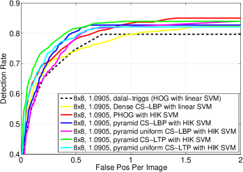
Figure 11: Detection rate versus false positive per-image (FPPI) curves for detectors based on the pyramid CS-LBP$/$LTP features using IKSVM classifier, the pyramid uniform CS-LBP$/$LTP features using IKSVM classifier, the PHOG feature using IKSVM classifier, the HOG feature using linear SVM classifier and the dense CS-LBP feature with linear SVM classifier. $8\times 8$ is the step size and $1.0905$ is the scale factor of the sliding detection window.

V-C Study on the features combined with the pyramid CS-LBP and PHOG

In this experiment, our main aim is to find out whether the combination of our feature with the PHOG feature can achieve better detection result or not. Feature Combination is a recent trend in class-level object recognition in computer vision. One efficient method is to combine the kernels corresponding to different features. The simplest method to combine several kernels is to average them. Gehler and Nowozin [36] pointed out that this simplest method is highly competitive with multiple kernel learning (MKL) [37] method and the method based on boosting approaches proposed in [36]. Here, We simply average the two kernels corresponding to the pyramid uniform CS-LBP feature and the PHOG feature as follows:

$$K_{\rm c}(v_{1},v_{2})=\tfrac{1}{2}[K_{1}(v_{1})+K_{2}(v_{2})],$$ (6)

where $K_{1}$ and $K_{2}$ are the IKSVMs classifiers pretrained using the pyramid uniform CS-LBP feature and the PHOG feature respectively, $v_{1}$ and $v_{2}$ are the pyramid uniform CS-LBP feature and the PHOG feature of a detection window respectively.

Detection performance are shown In Fig. 12. The detection rate versus FPPI curves show that the feature combination can significantly improve the detection performance. Compared to the PHOG, the detection rate raises about $6\%$ at 0.25 FPPI and raises about $1.5\%$ at 0.5 to 1 FPPI. Fig. 13 shows pedestrian detection on some example test images. The three rows show the bounding boxes detected by PHOG based detector, the pyramid uniform CS-LBP based detector and the PHOG + pyramid uniform CS-LBP based detector, respectively. We can see that the PHOG with pyramid uniform CS-LBP based detector performs best.

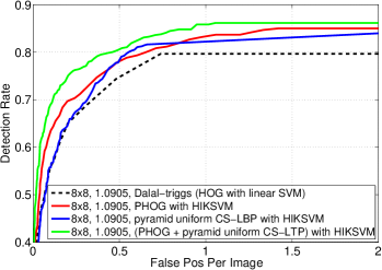
Figure 12: Detection rate versus false positive per-image(FPPI) curves for detectors(using IKSVM classifier) based on the PHOG features, the uniform CS-LBP feature and the augmented features combined by the HOG and the pyramid uniform CS-LBP. The augmented feature can improve the detection accuracy significantly. $8\times 8$ is the step size and $1.0905$ is the scale factor of the sliding detection window.

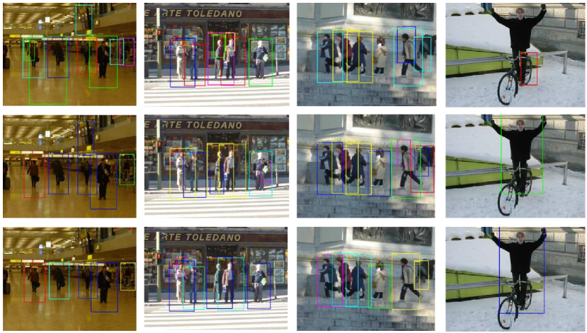
Figure 13: Some examples of detections on test images for the detectors using PHOG, pyramid uniform CS-LBP and augmented features (combined with HOG and pyramid uniform CS-LBP). First row: detected by the PHOG based detector. Second row: detected by the pyramid uniform CS-LBP based detector. Third row: detected by the PHOG+pyramid uniform CS-LBP based detector.

VI Conclusion

We have presented the dense CS-LBP feature and the pyramid CS-LBP$/$LTP features for pedestrian detection. Experimental results on the INRIA dataset show that the dense CS-LBP feature based approach the pyramid CS-LTP features using the IKSVM classifier outperform the PHOG, and the pyramid CS-LBP features perform as well as the HOG feature. We have also show that combining the pyramid CS-LBP with PHOG produces a significantly better detection performance on the INRIA dataset.

There are many directions for further research. To make the conclusion more convincing, the performance of the pyramid CS-LBP$/$LTP features based pedestrian detector needs to be further evaluated on other dataset, e.g., the Daimler Chrysler Pedestrian Dataset [11] and the Caltech Pedestrian Dataset [13]. Another further study is to compare the computational complexity of the pyramid CS-LBP$/$LTP features with PHOG both theoretically and experimentally. Thirdly, it is worthy studying how to combine our features with PHOG or other features more efficiently. We are also interested in implement the new feature in a boosting framework.

Yongbin Zheng is a Ph.D. student at the National University of Defense Technology, China and is currently visiting the Canberra Research Laboratory of NICTA (National ICT Australia) and the Australian National University. He received the B.E. degree and M.E. degree in Control Science from the National University of Defense Technology in 2004 and 2006. His research interests include pattern recognition, image processing and machine learning.

Chunhua Shen completed the Ph.D. degree from School of Computer Science, University of Adelaide, Australia in 2005; and the M.Phil. degree from Mathematical Sciences Institute, Australian National University, Australia in 2009. Since Oct. 2005, he has been working with the computer vision program, NICTA (National ICT Australia), Canberra Research Laboratory, where he is a senior research fellow and holds a continuing research position. His main research interests include statistical machine learning and its applications in computer vision and image processing.

Richard Hartley received the degree from the University of Toronto in 1976 with a thesis on knot theory. He is currently with the computer vision group at the Australian National University and also with NICTA (National ICT Australia), a government-funded research institute. He worked in this area for several years before joining the General Electric Research and Development Center, where he developed a computer-aided electronic design system called the Parsifal Silicon Compiler, described in his book “Digit Serial Computation”. Around 1990, he developed an interest in computer vision, and in 2000, he coauthored (with Andrew Zisserman) a book on multiple-view geometry. He has written papers on knot theory, geometric voting theory, computational geometry, computer-aided design, and computer vision. He holds 32 US patents. In 1991, he was awarded GE’s Dushman Award. He is a fellow of the IEEE and a member of the IEEE Computer Society.

Xinsheng Huang is a professor at the College of Mechatronics Engineering and Automation, the National University of Defense Technology, China. His research interests include control science, inertial navigation and image processing.

References

- [1] T. Ojala, M. Pietikainen, and D. Harwood, “A comparative study of texture meatures with classification based on featured distribution,” Pattern Recogn., vol. 29, no. 1, pp. 51–59, 1996.
- [2] I. Haritaoglu, D. Harwood, and L. S. Davis, “W4: real-time surveillance of people and their activities,” IEEE Trans. Pattern Anal. Mach. Intell., vol. 22, no. 8, pp. 809–830, 2000.
- [3] D. M. Gavrila and S. Munder, “Multi-cue pedestrian detection and tracking from a moving vehicle,” Int. J. Comp. Vis., vol. 73, no. 1, pp. 41–59, 2007.
- [4] D. M. G. abd J. Giebel and S. Munder, “Vision-based pedestrian detection: the protector system,” in Proc. IEEE Int. Conf. Intell. Vehic. Symposium, Parma, Italy, 2004, pp. 13–18.
- [5] T.Nakada, S.Kagami, and H.Mizoguchi, “Pedestrian detection using 3d optical flow sequences for a mobile robot,” in Proc. IEEE Conf. Sens., Leece, Italy, 2008, pp. 776–779.
- [6] P. Viola, M. J. Jones, and D. Snow, “Detecting pedestrian using patterns of motion and appearance,” in Proc. IEEE Int. Conf. Comp. Vis., vol. 2, Nice, France, 2003, pp. 734–741.
- [7] K. Mikolajczyk, C. Schmid, and A. Zisserman, “Human detection based on a probabilistic assembly of robust part detectors,” in Proc. Eur. Conf. Comp. Vis., vol. 3021/2004, LNCS, Prague, Czech Republic, 2004, pp. 69–82.
- [8] N. Dalal and B. Triggs, “Histogram of oriented gradients for human detection,” in Proc. IEEE Conf. Comp. Vis. Patt. Recogn., vol. 1, San Diego, USA, 2005, pp. 886–893.
- [9] N. Dalal, “Finding people in images and videos,” Ph.D. dissertation, Institut National Polytechnique de Grenoble, 2006.
- [10] O. Tuzel, F. Porikli, and P. Meer, “Human detection via classification on riemannian manifolds,” in Proc. IEEE Conf. Comp. Vis. Patt. Recogn., Minneapolis, Minnesota, USA, 2007, pp. 1–8.
- [11] S. Munder and D. M. Gavrila, “An experimental study on pedestrian classification,” IEEE Trans. Pattern Anal. Mach. Intell., vol. 28, no. 11, pp. 1863–1868, 2006.
- [12] S. Paisitkriangkrai, C. Shen, and J. Zhang, “Fast pedestrian detection using a cascade of boosted covariance features,” IEEE Trans. Circuits Syst. Video Technol., vol. 18, no. 8, pp. 1140–1151, 2008.
- [13] P. Dollár, C. Wojek, B. Schiele, and P. Perona, “Pedestrian detection: A benchmark,” in Proc. IEEE Conf. Comp. Vis. Patt. Recogn., 2009, pp. 304–311.
- [14] X. Wang, T. Han, and S. Yan, “An HoG–LBP human detector with partial occlusion handling,” in Proc. IEEE Int. Conf. Comp. Vis., Kyoto, Japan, 2009, pp. 32–39.
- [15] M. Enzweiler and D. M. Gavrila, “Monocular pedestrian detection: Survey and experiments.” IEEE Trans. Pattern Anal. Mach. Intell., vol. 31, no. 12, pp. 2179–2195, 2009.
- [16] M. Enzweiler, A. Eigenstetter, B. Schiele, and D. M. Gavrila, “Multi-cue pedestrian classification with partial occlusion handling,” in Proc. IEEE Conf. Comp. Vis. Patt. Recogn., 2010.
- [17] B. Leibe, E. Seemann, and B. Schiele, “Pedestrian detection in crowded scenes,” in Proc. IEEE Conf. Comp. Vis. Patt. Recogn., vol. 1, 2005, pp. 878–885.
- [18] P. Sabzmeydani and G. Mori, “Detecting pedestrians by learning shapelet features,” in Proc. IEEE Conf. Comp. Vis. Patt. Recogn., Minneapolis, Minnesota, USA, 2007, pp. 1–8.
- [19] Q. Zhu, S. Avidan, M.-C. Yeh, and K.-T. Cheng, “Fast human detection using a cascade of histograms of oriented gradients,” in Proc. IEEE Conf. Comp. Vis. Patt. Recogn., vol. 2, New York City, USA, 2006, pp. 1491–1498.
- [20] S. Maji, A. Berg, and J. Malik, “Classification using intersection kernel support vector machines is efficient,” in Proc. IEEE Conf. Comp. Vis. Patt. Recogn., Anchorage, Alaska, USA, 2008, pp. 1–8.
- [21] I. P. Alonso, D. F. Llorca, and M. A. Sotelo, “Combination of feature extraction methods for svm pedestrian detection,” Trans. Intell. Transp. Syst., vol. 8, no. 2, pp. 292–307, 2007.
- [22] C. Wojek, S. Walk, and B. Schiele, “Multi-cue onboard pedestrian detection,” in Proc. IEEE Conf. Comp. Vis. Patt. Recogn., Miami, Florida, USA, 2009, pp. 794–801.
- [23] C. Shen and H. Li, “On the dual formulation of boosting algorithms,” IEEE Trans. Pattern Anal. Mach. Intell., Published online: 18 March, 2010. [Online]. Available: http://dx.doi.org/10.1109/TPAMI.2010.47
- [24] M. Heikkila and C. Schmid, “Description of interest regions with local binary patterns,” Pattern Recogn., vol. 42, no. 3, pp. 425–436, 2009.
- [25] T. Ojala, M. Pietikainen, and T. Maenpaa, “Multiresolution gray-scale and rotation invariant texture classification with local binary patterns,” IEEE Trans. Pattern Anal. Mach. Intell., vol. 24, no. 7, pp. 971–987, 2002.
- [26] T. Ahonen, A. Hadid, and M. Pietikainen, “Face detection with local binary patterns: application to face recognition,” IEEE Trans. Pattern Anal. Mach. Intell., vol. 28, no. 12, pp. 2037–2041, 2006.
- [27] X. Tan and B. Triggs, “Enhanced local texture feature sets for face recognition under difficult lighting conditions,” IEEE Trans. Image Process., vol. 19, no. 6, pp. 1635–1650, 2010.
- [28] D. W. Lowe, “Distinctive image features from scale-invariant keypoints,” Int. J. Comp. Vis., vol. 60, no. 2, pp. 91–110, 2004.
- [29] D. Comaniciu and P. Meer, “Mean shift: A robust approach toward feature space analysis,” IEEE Trans. Pattern Anal. Mach. Intell., vol. 24, no. 5, pp. 603–619, 2002.
- [30] A. Bosch, A. Zisserman, and X. Munoz, “Scene classification via PLSA,” in Proc. Eur. Conf. Comp. Vis., vol. 3954/2006, LNCS, Graz, Austria, 2006, pp. 517–530.
- [31] ——, “Representing shape with a spatial pyramid kernel,” in Proc. ACM. Int. Conf. Image & video retrieval, 2007, pp. 401–408.
- [32] M. J. Swain and D. H. Ballard, “Color indexing,” Int. J. Comp. Vis., vol. 7, no. 1, pp. 11–32, 1991.
- [33] F. Odone, A. Barla, and A. Verri, “Building kernels from binary strings for image matching,” IEEE Trans. Image Process., vol. 14, no. 2, pp. 169–180, 2005.
- [34] S. Maji and A. C. Berg, “Max-margin additive classifiers for detection,” in Proc. IEEE Int. Conf. Comp. Vis., 2009, pp. 40–47.
- [35] C.-C. Chang and C.-J. Lin, LIBSVM: a library for support vector machines, 2001, software available at http://www.csie.ntu.edu.tw/~cjlin/libsvm.
- [36] P. Gehler and S. Nowozin, “On feature combination for multiclass object classification,” in Proc. IEEE Int. Conf. Comp. Vis., 2009, pp. 221–228.
- [37] F. Bach, G. R. G. Lanckriet, and M. I. Jordan, “Multiple kernel learning, conic duality, and the smo algorithm,” in Proc. Int. Conf. Mach. Learn., Banff, Alberta, Canada, 2004.