Current Developments in Nuclear Density Functional Methods

Abstract

Density functional theory (DFT) became a universal approach to compute ground-state and excited configurations of many-electron systems held together by an external one-body potential in condensed-matter, atomic, and molecular physics. At present, the DFT strategy is also intensely studied and applied in the area of nuclear structure. The nuclear DFT, a natural extension of the self-consistent mean-field theory, is a tool of choice for computations of ground-state properties and low-lying excitations of medium-mass and heavy nuclei. Over the past thirty-odd years, a lot of experience was accumulated in implementing, adjusting, and using the density-functional methods in nuclei. This research direction is still extremely actively pursued. In particular, current developments concentrate on (i) attempts to improve the performance and precision delivered by the nuclear density-functional methods, (ii) derivations of density functionals from first principles rooted in the low-energy chromodynamics and effective theories, and (iii) including effects of low-energy correlations and symmetry restoration. In this study, we present an overview of recent results and achievements gained in nuclear density-functional methods.

1 Introduction

The Density Functional Theory (DFT) was introduced in atomic physics through the Hohenberg-Kohn [1] and Kohn-Sham [2] theorems. Its quantum-mechanical foundation relies on a simple variational concept that uses observables as variational parameters. Namely, for any Hamiltonian $\hat{H}$ and observable $\hat{Q}$, one can formulate the constraint variational problem,

$$\delta\langle\hat{H}-\lambda\hat{Q}\rangle=0,$$ (1)

whereby the total energy of the system $E\equiv\langle\hat{H}\rangle$ becomes a function of the observable $Q\equiv\langle\hat{Q}\rangle$, that is $E=E(Q)$, provided the Lagrange multiplier $\lambda$ can be eliminated from functions $E(\lambda)$ and $Q(\lambda)$ that are obtained from the variation in Eq. (1) performed at fixed $\lambda$. This can be understood in terms of a two-step variational procedure. First, Eq. (1) ensures that the total energy is minimized at fixed $Q$, and second, the minimization of $E(Q)$ in function of $Q$ gives obviously the exact ground-state energy $E_{0}=\min_{Q}E(Q)$ and the exact value $Q_{0}$ of the observable $Q$ calculated for the ground-state wave function.

Function $E(Q)$ is thus the simplest model of the density functional. However, the idea of two-step variational procedure can be applied to an arbitrary observable or a set of observables, and hence the total energy can become a function $E(Q_{k})$ of several observables $Q_{k}$, $\delta\langle\hat{H}-\sum_{k}\lambda_{k}\hat{Q}_{k}\rangle=0\Longrightarrow E=E(Q_{k})$, or a functional $E[Q(q)]$ of a continuous set of observables $Q(q)$, $\delta\langle\hat{H}-\int\rmd q\,\lambda(q)\hat{Q}(q)\rangle=0\Longrightarrow E=E[Q(q)]$.

When these ideas are applied to the observable $\hat{\rho}({\mathbf{r}})=\sum_{i=1}^{A}\delta({\mathbf{r}}-{\mathbf{r}}_{i})$, which is the local density of a many-body system at point ${\mathbf{r}}$, we obtain the original local DFT,

$$\delta\langle\hat{H}-\int\rmd{\mathbf{r}}\,V({\mathbf{r}})\hat{\rho}({\mathbf{r}})\rangle=0~{}~{}~{}~{}\Longrightarrow~{}~{}~{}~{}E=E[\rho({\mathbf{r}})],$$ (2)

whereby the local external potential $V({\mathbf{r}})$ plays the role of the Lagrange multiplier that selects a given density profile ${\rho}({\mathbf{r}})$. By the same token, the nonlocal DFT is obtained by using a nonlocal external potential $V({\mathbf{r}},{\mathbf{r}}\,^{\prime})$,

$$\delta\langle\hat{H}-\int\rmd{\mathbf{r}}\int\rmd{\mathbf{r}}\,^{\prime}\,V({\mathbf{r}},{\mathbf{r}}\,^{\prime})\hat{\rho}({\mathbf{r}},{\mathbf{r}}\,^{\prime})\rangle=0~{}~{}~{}~{}\Longrightarrow~{}~{}~{}~{}E=E[\rho({\mathbf{r}},{\mathbf{r}}\,^{\prime})].$$ (3)

In each of these cases, by minimizing the functionals $E[\rho({\mathbf{r}})]$ or $E[\rho({\mathbf{r}},{\mathbf{r}}\,^{\prime})]$, we obtain the exact ground-state energy of the many-body system along with its exact local ${\rho}({\mathbf{r}})$ or nonlocal $\rho({\mathbf{r}},{\mathbf{r}}\,^{\prime})$ one-body density.

It is thus obvious that the idea of two-step variational principle, which is at the heart of DFT, does not give us any hint on which observable has to be picked as the variational parameter. Moreover, the exact derivation of the density functional is entirely impractical, because it involves solving exactly the variational problem that is equivalent to finding the exact ground state. If we were capable of doing that, no DFT would have been further required. Nevertheless, the exact arguments presented above can serve us as a justification of modelling the ground-state properties of many-body systems by DFT, which, however, must be rather guided by physical intuition, general theoretical arguments, experiment, and exact calculations for simple systems.

2 Fundamentals

An example that highlights connection with ab-initio theory is shown in Fig. 1, Ref. [3], where binding energies calculated exactly for neutron drops confined within the Woods-Saxon potential of two different depths, $V_{0}=-25$ and $-35.5$ MeV, are compared with those corresponding to several Skyrme functionals [4]. Calculations of this type, performed at different depths, surface thicknesses, and deformations of the confining potential may allow for a better determination of Skyrme-functional parameters.

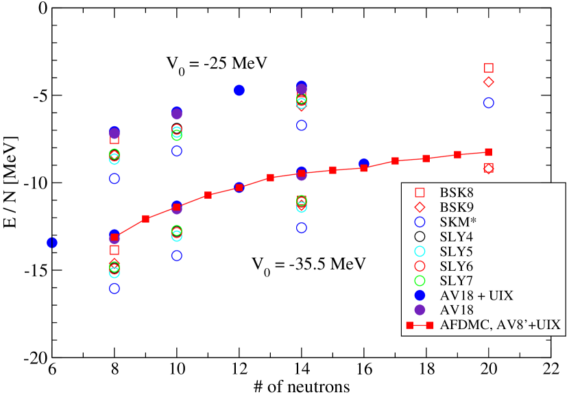
Figure 1: Energies of neutron drops confined by the Woods-Saxon potential, see the text. From Ref. [3]; picture courtesy of R.B. Wiringa.

In practice, the exact density functionals (2) or (3) are modelled as integrals of energy densities ${\cal H}$, and thus they are called energy-density functionals (EDFs). They can be local functions of local densities (4), quasilocal functions of local higher-order densities (5), nonlocal functions of local densities (6), or nonlocal functions of nonlocal densities (7).

$$E[\rho({\mathbf{r}})] \!\!\!\!=\!\!\!\! \!\!\int\!\!\rmd{\mathbf{r}}\,{\cal H}(\rho({\mathbf{r}})),$$ (4)

$$E[\rho({\mathbf{r}})] \!\!\!\!=\!\!\!\! \!\!\int\!\!\rmd{\mathbf{r}}\,{\cal H}(\rho({\mathbf{r}}),\tau({\mathbf{r}}),\Delta\rho({\mathbf{r}}),\ldots),$$ (5)

$$E[\rho({\mathbf{r}})] \!\!\!\!=\!\!\!\! \!\!\int\!\!\rmd{\mathbf{r}}\!\!\int\!\!\rmd{\mathbf{r}}\,^{\prime}\,{\cal H}(\rho({\mathbf{r}}),\rho({\mathbf{r}}\,^{\prime})),$$ (6)

$$E[\rho({\mathbf{r}},{\mathbf{r}}\,^{\prime})] \!\!\!\!=\!\!\!\! \!\!\int\!\!\rmd{\mathbf{r}}\!\!\int\!\!\rmd{\mathbf{r}}\,^{\prime}\,{\cal H}(\rho({\mathbf{r}},{\mathbf{r}}\,^{\prime})).$$ (7)

Two major classes of approach that are currently used and developed in nuclear structure physics are based on relativistic and nonrelativistic EDFs [5, 4, 6]. The nonrelativistic EDFs are most often built as:

$${\cal H}(\rho({\mathbf{r}},{\mathbf{r}}\,^{\prime}))={1\over 2}\sum_{vt}\left(\hat{V}^{\mbox{\rm{\scriptsize{dir}}}}_{vt}({\mathbf{r}},{\mathbf{r}}\,^{\prime})\left[\left[\rho^{t}_{v}({\mathbf{r}})\rho^{t}_{v}({\mathbf{r}}\,^{\prime})\right]^{0}\right]_{0}-\hat{V}^{\mbox{\rm{\scriptsize{exc}}}}_{vt}({\mathbf{r}},{\mathbf{r}}\,^{\prime})\left[\left[\rho^{t}_{v}({\mathbf{r}},{\mathbf{r}}\,^{\prime})\rho^{t}_{v}({\mathbf{r}}\,^{\prime},{\mathbf{r}})\right]^{0}\right]_{0}\right),$$ (8)

where $\hat{V}^{\mbox{\rm{\scriptsize{dir}}}}_{vt}$ and $\hat{V}^{\mbox{\rm{\scriptsize{exc}}}}_{vt}$ denote the EDF-generating (pseudo)potentials in the direct and exchange channels, respectively, and we sum over the spin-rank $v=0$ and 1 (scalar and vector) and isospin-rank $t=0$ and 1 (isoscalar and isovector) spherical-tensor densities [7, 8] coupled to the total isoscalar (superscript 0) and scalar (subscript 0) term. For example, finite-range momentum-independent central potentials generate the Gogny [9] or M3Y [10] nonlocal functionals (8) and zero-range momentum-dependent pseudopotentials generate the Skyrme [4] or BCP [11] quasilocal functionals (6).

Expression (8) derives from the Hartree-Fock formula for the average energy of a Slater determinant. However, the EDF-generating pseudopotentials should not be confused with the nucleon-nucleon (NN) bare or effective interaction or Brueckner G-matrix. Indeed, their characteristic features are different – they neither are meant to describe the NN scattering properties, as the bare NN force is, nor are meant to be used in a restricted phase space, as the effective interaction is, nor depend on energy, as the G-matrix does. Moreover, to ensure correct saturation properties, the EDF-generating pseudopotentials must themselves depend on the density. But most importantly, the generated EDFs are modelled so as to describe the exact binding energies and not those in the Hartree-Fock approximation, which otherwise would have required adding higher-order corrections based on the many-body perturbation theory.

Only very recently, it has been demonstrated [12, 8] that the nuclear nonlocal EDFs, based on sufficiently short-range EDF-generating pseudopotentials, are equivalent to quasilocal EDFs. In Fig. 2 are compared the proton RMS radii and binding energies of doubly magic nuclei, determined by using the Gogny D1S EDF [13] and second-order Skyrme-like EDF S1Sb [12] derived therefrom by using the Negele-Vautherin (NV) density-matrix expansion (DME) [14]. One can see that already at second order, the DME gives excellent precision of the order of 1%. In Ref. [15], similar conclusions were also reached when comparing the nonlocal and quasilocal relativistic EDFs, see Fig. 3.

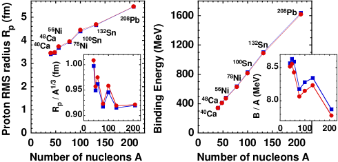
Figure 2: Proton RMS radii (left) and binding energies (right) of doubly magic nuclei, determined by using the Gogny D1S EDF [13] (squares) and second-order Skyrme-like EDF [12] derived therefrom (circles). The insets show results in expanded scales and scaled by particle numbers $A$.

Figs. 5 and 5 show convergence of the direct and exchange interaction energies, respectively, when the Taylor and damped Taylor (DT) DMEs are performed up to sixth order [8]. The four panels of Fig. 5 show results obtained in the four spin-isospin channels labeled by $V_{vt}$. Results of the DT DME [8] are compared with those corresponding to the NV [14] and PSA [16] expansions. It is extremely gratifying to see that in each higher order the precision increases by a large factor, which is characteristic to a rapid power-law convergence. The success and convergence of the DME expansions relies on the fact that the finite-range nuclear effective interactions are very short-range as compared to the spatial variations of nuclear densities. The quasilocal (gradient) expansion in nuclei works!

Figure 3: The relative deviations (in percentages) between the experimental and theoretical charge radii (upper panel) and binding energies (lower panel) of 12 spherical nuclei, calculated with the meson-exchange interaction DD-ME2 and the four point-coupling parameter sets. In all cases, the relative deviations are below 1%. Starting from the meson-exchange density-dependent interaction DD-ME2, the equivalent point-coupling parametrization for the effective Lagrangian was derived by incorporating the density dependence of the parameters. The parameters of the point-coupling model were adjusted to reproduce the nuclear matter equation of state obtained with the DD-ME2 interaction and surface thickness and surface energy of semi-infinite nuclear matter. Reprinted figure with permission from Ref. [15]. Copyright 2008 by the American Physical Society.

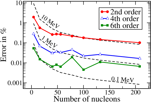
Figure 4: Precision of the Taylor DME of the direct interaction energies calculated for the nonlocal Gogny D1S EDF [17]. The nine nuclei used for the test are ⁴He, ¹⁶O, ^40,48Ca, ^56,78Ni, ^100,132Sn, and ²⁰⁸Pb. From Ref. [8].

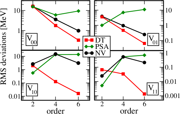
Figure 5: The RMS deviations between the exact and approximate exchange energies calculated for the nine nuclei listed in the caption of Fig. 5, see the text. From Ref. [8].

3 Applications

When compared to the experimental binding energies, the quasilocal Skyrme functional HFB-17 [18] (Fig. 7) gives results, which have the quality very similar to those given by the nonlocal Gogny functional D1M [19] (Fig. 7). In both cases, the functionals were augmented by terms responsible for the pairing correlations and all parameters were adjusted specifically to binding energies. Moreover, in both cases, by using either the 5D collective Hamiltonian approach or configuration mixing, theoretical binding energies were corrected for collective quadrupole correlations. The results are truly impressive, with the RMS deviations calculated for 2149 masses being as small as 798 and 581 keV, respectively.

Figure 6: Differences between measured [20] and HFB-17 [18] masses, as a function of the neutron number $N$. Reprinted figure with permission from Ref. [18]. Copyright 2009 by the American Physical Society.

Figure 7: Differences between measured [20] and D1M [19] masses, as a function of the neutron number $N$. Reprinted figure with permission from Ref. [19]. Copyright 2009 by the American Physical Society.

The problem of treating collective correlations and excitations within the DFT or EDF approaches is one of the most important issues currently studied in applications to nuclear systems. The question of whether one can describe these effects by using the functional only is not yet resolved. In practice, relatively simple functionals that are currently in use, require adding low-energy correlation effects explicitly. This can be done by reverting from the description in terms of one-body densities back to the wave functions of mean-field states. For example, for quadrupole correlations this amounts to using the following configuration-mixing states,

$$|\Psi_{NZ,JM}\rangle=\int\rmd\beta\rmd\gamma\sum_{K}f_{K}(\beta,\gamma)\hat{P}_{N}\hat{P}_{Z}\hat{P}_{JMK}|\Psi(\beta,\gamma)\rangle,$$ (9)

where $\hat{P}_{N}$, $\hat{P}_{Z}$, and $\hat{P}_{JMK}$ are projection operators on good neutron number $N$, proton number $Z$, and angular momentum $J$ with laboratory and intrinsic projections $M$ and $K$. The intrinsic mean-field wave functions $|\Psi(\beta,\gamma)\rangle$ correspond to one-body densities constrained to quadrupole deformations $\beta$ and $\gamma$ [21].

To determine variationally the mixing amplitudes $f_{K}(\beta,\gamma)$, one has to generalize the energy densities, such as those shown in Eqs. (4)–(7), to transition energy densities that enable us to compute Hamiltonian kernels. For mean-field states, this can be rigorously done by using the Wick theorem, whereby the average energy $\langle\Psi|\hat{H}|\Psi\rangle$ generalizes to matrix element $\langle\Psi_{1}|\hat{H}|\Psi_{2}\rangle$ as [21]:

$$\langle\Psi|\hat{H}|\Psi\rangle \simeq \int\rmd{\mathbf{r}}\int\rmd{\mathbf{r}}\,^{\prime}\,{\cal H}(\rho({\mathbf{r}},{\mathbf{r}}\,^{\prime}))~{}~{}~{}~{}\mbox{for}~{}~{}\rho({\mathbf{r}},{\mathbf{r}}\,^{\prime})={\displaystyle\frac{\langle\Psi|a^{+}({\mathbf{r}}\,^{\prime})a({\mathbf{r}}\,^{\prime})|\Psi\rangle}{\langle\Psi|\Psi\rangle}},$$ (10)

$$\langle\Psi_{1}|\hat{H}|\Psi_{2}\rangle \simeq \int\rmd{\mathbf{r}}\int\rmd{\mathbf{r}}\,^{\prime}\,{\cal H}(\rho_{12}({\mathbf{r}},{\mathbf{r}}\,^{\prime}))~{}~{}~{}~{}\mbox{for}~{}~{}\rho_{12}({\mathbf{r}},{\mathbf{r}}\,^{\prime})={\displaystyle\frac{\langle\Psi_{1}|a^{+}({\mathbf{r}}\,^{\prime})a({\mathbf{r}}\,^{\prime})|\Psi_{2}\rangle}{\langle\Psi_{1}|\Psi_{2}\rangle}}.$$ (11)

Although for densities of correlated states, which are employed in DFT or EDF methods, this prescription cannot be properly justified, it has been successfully used in many practical applications. However, even this simple prescription creates problems [22], which may require implementing more complicated schemes [23].

Figure 8: Scatter plot comparing the theoretical and experimental $2^{+}_{1}$ excitation energies of the 359 nuclei included in the survey of Ref. [24]; picture courtesy of M. Bender.

Figure 9: Theoretical $2^{+}_{1}$ excitation energies of 537 even-even nuclei as a function of their experimental values [25]. Reprinted figure with permission from Ref. [13]. Copyright 2010 by the American Physical Society.

An example of the results is shown in Fig. 9, where calculated $2^{+}_{1}$ excitation energies [24] are compared with experimental data. One obtains fairly good description for nuclei across the nuclear chart. Calculations slightly overestimate the data, which is most probably related to the fact that in this study the nonrotating mean-field states were used, see Ref. [26] and references cited therein. As shown in Fig. 9, this deficiency disappears when the moments of inertia of the 5D collective Hamiltonian are determined by using infinitesimal rotational frequencies [13]. At present, calculations using in light nuclei the triaxial projected states of Eq. (9) are becoming possible for the relativistic (Fig. 11) and quasilocal (Fig. 11) functionals.

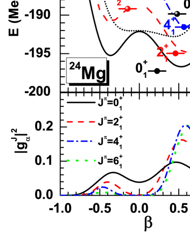
Figure 10: Energies and the average axial deformations for the two lowest quadrupole states with angular momenta 0⁺, 2⁺, 4⁺, and 6⁺ in ²⁴Mg, together with the mean-field (dotted) and the corresponding angular-momentum-projected energy curves and squares of collective wave functions. Reprinted figure with permission from Ref. [27]. Copyright 2010 by the American Physical Society.

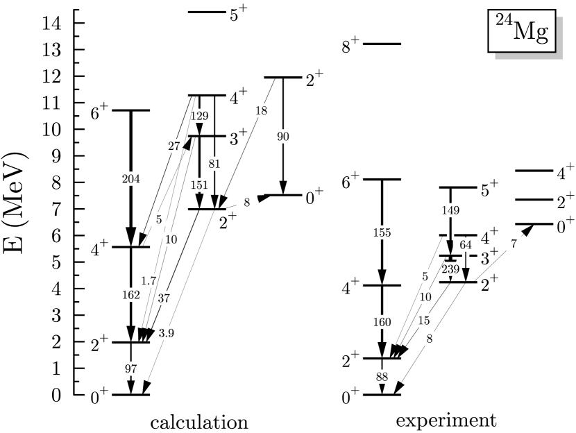
Figure 11: Excitation spectra and B(E2) values in e² fm⁴ compared to the available experimental data in ²⁴Mg. The spectrum is subdivided into a ground-state band, a $\gamma$ band, and additional low-lying states that do not necessarily form a band. From Ref. [28]; picture courtesy of M. Bender.

Another fascinating collective phenomenon that can presently be described for the non-local [29, 30] and quasilocal functionals [31] is the fission of very heavy nuclei. In Fig. 13, an example of fission-path calculations performed in ²⁵⁸Fm is shown in function of the elongation and shape-asymmetry parameters. One obtains correct description of the region of nuclei where the phenomenon of bimodal fission occurs and predicts regions of the trimodal fission, see Fig. 13.

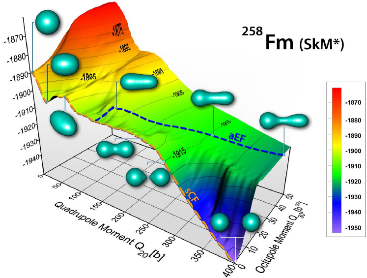
Figure 12: The energy surface of ²⁵⁸Fm calculated for the quasilocal EDF as a function of two collective variables: the total quadrupole moment $Q_{20}$ representing the elongation of nuclear shape, and the total octupole moment $Q_{30}$ representing the left-right shape asymmetry. Indicated are the two static fission valleys: asymmetric path aEF and symmetric-compact path sCF. From Ref. [32]; picture courtesy of A. Staszczak.

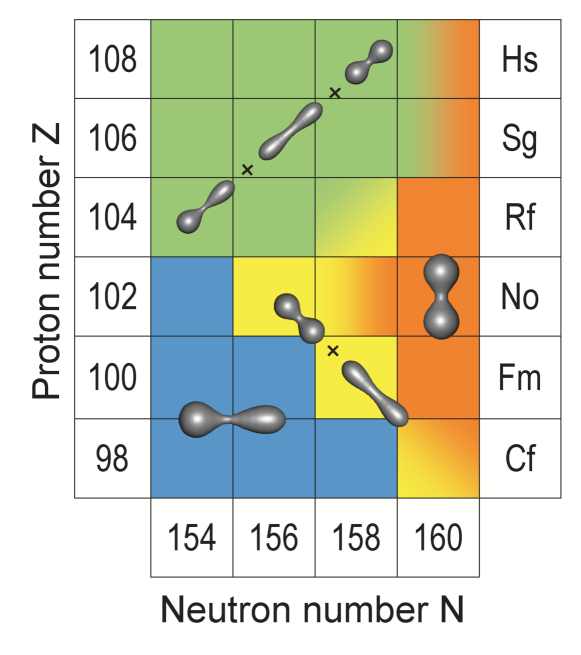
Figure 13: Summary of fission pathway results obtained in Ref. [31]. Nuclei around ²⁵²Cf are predicted to fission along the asymmetric path and those around ²⁶²No along the symmetric path. These two regions are separated by the bimodal symmetric fission around ²⁵⁸Fm. In a number of the Rf, Sg, and Hs nuclei, all three fission modes are likely (trimodal fission). From Ref. [31]

In recent years, significant progress was achieved in determining the multipole giant resonances in deformed nuclei by using the RPA and QRPA methods. In light nuclei, the multipole modes can be determined for the nonlocal, relativistic, and quasilocal functionals, see Figs. 15, 15, and 17, respectively. In heavy nuclei, such calculations are very difficult, because the number of two-quasiparticle configurations that must be taken into account grows very fast with the size of the single-particle phase space. Nevertheless, the first calculation of this kind has already been reported for ¹⁷²Yb, see Fig. 17. The future developments here will certainly rely on the newly developed iterative methods of solving the RPA and QRPA equations [33, 34, 35].

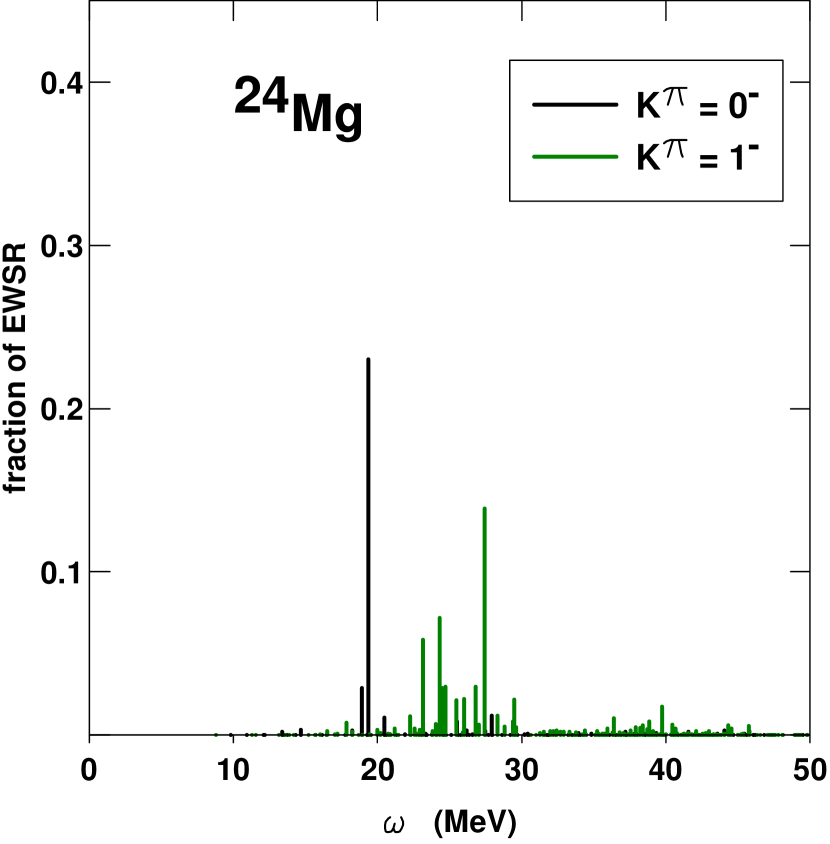
Figure 14: Dipole excitations in ²⁴Mg determined for the nonlocal Gogny D1S functional. From Ref. [36]; picture courtesy of S. Péru.

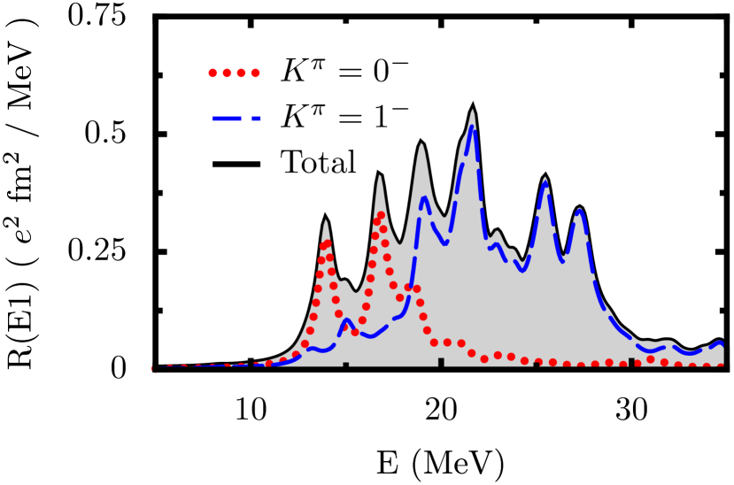
Figure 15: Dipole excitations in ²⁰Ne determined for the relativistic NL3 functional. Reprinted figure with permission from Ref. [37]. Copyright 2008 by the American Physical Society.

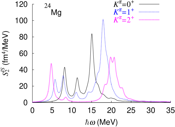
Figure 16: Quadrupole excitations in ²⁴Mg determined for the quasilocal Skyrme SkM* functional. Reprinted figure with permission from Ref. [38]. Copyright 2008 by the American Physical Society.

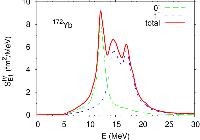
Figure 17: Dipole excitations in ¹⁷²Yb determined for the quasilocal Skyrme SkM* functional. From Ref. [39]; picture courtesy of J. Terasaki.

The EDF methods were also recently applied within the full 3D dynamics based on the time-dependent mean-field approach. In Ref. [40], the spin-independent transition density was calculated in the 3D coordinate space for the time-dependent dipole oscillations. It turned out that one of the Steinwedel-Jensen’s assumptions [41], $\delta\rho_{n}({\mathbf{r}};t)=-\delta\rho_{p}({\mathbf{r}};t)$, was approximately satisfied for ⁸Be. In contrast, in ¹⁴Be, large deviation from this property was noticed. Figure 19 shows how transition densities $\delta\rho_{n}({\mathbf{r}};t)$ (lower panels) and $\delta\rho_{p}({\mathbf{r}};t)$ (upper panels) evolve in time in the $x$–$z$ plane. The time difference from one panel to the next (from left to right) roughly corresponds to the half oscillation period. White (black) regions indicate those of positive (negative) transition densities. One sees that significant portions of neutrons actually move in phase with protons.

An interesting 3D EDF time-dependent calculation was recently performed for the $\alpha$–⁸Be fusion reaction [42]. Although this calculation aimed at elucidating properties of the triple-$\alpha$ reaction, it was performed at the energy above the barrier, where the time-dependent mean-field approach can lead to fusion, whereas the real triple-$\alpha$ reaction involves tunneling through the Coulomb barrier. Nevertheless, the studied tip-on initial configuration in the entrance channel, shown in the upper panel of Fig. 19, is probably the preferred one as it must correspond to the lowest barrier. The calculations lead to the formation of a metastable linear chain state of three $\alpha$-like clusters which subsequently made a transition to a lower-energy triangular $\alpha$-like configuration before acquiring a more compact final shape, as shown in the lower panels of Fig. 19.

Figure 18: Nuclear TDHF transition densities in ¹⁴Be, see the text. Reprinted from Ref. [40], Copyright 2007, with permission from Elsevier.

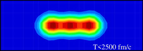
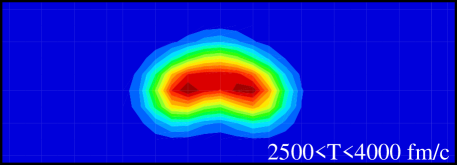
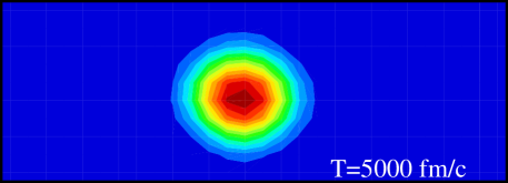
Figure 19: Nuclear TDHF densities in ¹⁴Be, see the text. Reprinted figure with permission from Ref. [42]. Copyright 2010 by the American Physical Society.

4 Conclusions

The EDF methods are presently very intensely studied and developed in nuclear physics. Apart from the subjects covered in the present short review, there is a number of topics that could not be discussed here, such as: formal aspects of the DFT for self-bound systems; symmetry breaking effects; ab initio derivation of the EDF from the chiral perturbation and Brueckner-Hartree-Fock theories; studies of weakly-bound systems and the continuum phase-space effects; functionals non-local in time and the adiabatic connection; new-generation functionals with higher-order derivatives and/or richer density dependencies; self-interactions and self-pairing in the EDF; and ambiguities and inconsistencies when extending the EDF methods to multi-reference applications.

Moreover, there are several aspects related to the methodology that were not covered here, such as: the EDF methods based on natural occupation numbers and/or orbitals; second, extended, and/or self-consistent (Q)RPA methods; proton-neutron interactions and isovector terms in the EDF; extrapolations to exotic nuclei and astrophysical applications; equation of state, symmetry energy, and neutron stars; relations between functionals describing infinite systems and finite nuclei; and adjustments of parameters, confidence intervals, and correlations.

There is also a number of other interesting applications of the nuclear EDF methods, such as: description of tensor effects and the spin-orbit splitting; functionals describing pairing correlations; particle-vibration coupling, single-particle spectra, and widths of giant resonances; fusion barriers and cross sections within static and time-dependent calculations; fermion systems in the unitary regime; neutron skins and pygmy resonances; time-odd terms versus spin and orbital M1 resonances, spin-isospin resonances, and particle-vibration coupling and polarization; incompressibility, effective mass, and monopole resonances; cluster structures and models; chirality in rotational bands; di-neutron correlations and deformation in nuclear halos; and Coulomb frustration effects in the superheavy nuclei and crust of neutron stars.

In general, the EDF methods provide us with universal understanding of global low-energy nuclear properties and feature an impressive array of applications. These methods can be rooted in the effective-theory approach whereupon the low-energy phenomena can be successfully modeled without resolving high-energy properties. Further progress strongly relies upon the use of high-power computing and faces the challenge of working out a consistent scheme of consecutive corrections that would allow for the increased precision and predictive power.

During preparation of this talk, I have received suggestions and comments from very many of my colleagues; I would like to thank them very much for their help. In particular, I would like to thank: Michael Bender, Karim Bennaceur, George Bertsch, Aurel Bulgac, Rick Casten, Willem Dickhoff, Jerzy Dudek, Nguyen Van Giai, Bertrand Giraud, Elvira Moya de Guerra, Paul-Henri Heenen, Morten Hjorth-Jensen, Pieter Van Isacker, Jan Kvasil, Denis Lacroix, Elena Litvinova, Jérôme Margueron, Joachim Maruhn, Jie Meng, Witek Nazarewicz, Thomas Papenbrock, Michael Pearson, Jorge Piekarewicz, Nathalie Pillet, Marek Płoszajczak, Paul-Gerhard Reinhard, Peter Ring, Wojciech Satuła, Paul Stevenson, Sait Umar, James Vary, and Dario Vretenar.

This work was supported by the Academy of Finland and University of Jyväskylä within the FIDIPRO program, by the Polish Ministry of Science and Higher Education under Contract No. N N 202 328234, and by the U.S. Department of Energy under Contract No. DE-FC02-09ER41583 (UNEDF SciDAC Collaboration).

References

References

- [1] P Hohenberg and W Kohn, Phys Rev 136, B864 (1964)
- [2] W Kohn and LJ Sham, Phys Rev 140, A1133 (1965)
- [3] J Carlson, S Gandolfi, RB Wiringa, and the UNEDF Collaboration, http://unedf.org/, unpublished
- [4] M Bender, P-H Heenen, and P-G Reinhard, Rev Mod Phys 75, 121 (2003)
- [5] P Ring, Prog Part Nucl Phys 37, 193 (1996)
- [6] GA Lalazissis, P Ring, and D Vretenar (Eds) Extended Density Functionals in Nuclear Structure Physics, Lecture Notes in Physics Vol 641 (Springer Verlag, 2004)
- [7] BG Carlsson, J Dobaczewski, and M Kortelainen, Phys Rev C 78, 044326 (2008); 81, 029904(E) (2010)
- [8] BG Carlsson and J Dobaczewski, arXiv:1003.2543, Phys Rev Lett, in press
- [9] J Dechargé and D Gogny, Phys Rev C21, 1568 (1980)
- [10] H Nakada, Phys Rev C 68, 014316 (2003)
- [11] M Baldo, P Schuck, and X Viñas, Phys Lett B663, 390 (2008)
- [12] J Dobaczewski, BG Carlsson, and M Kortelainen, J Phys G: Nucl Part Phys 37, 075106 (2010)
- [13] J-P Delaroche, M Girod, J Libert, H Goutte, S Hilaire, S Péru, N Pillet, and GF Bertsch, Phys Rev C 81, 014303 (2010)
- [14] JW Negele and D Vautherin, Phys Rev C 5, 1472 (1972)
- [15] T Nikšić, D Vretenar, GA Lalazissis, and P Ring, Phys Rev C 77, 034302 (2008)
- [16] B Gebremariam, T Duguet, and SK Bogner, Phys Rev C 82, 014305 (2010)
- [17] J-F Berger, M Girod, and D Gogny, Comput Phys Comm 63, 365 (1991)
- [18] S Goriely, N Chamel, and J M Pearson, Phys Rev Lett 102, 152503 (2009)
- [19] S Goriely, S Hilaire, M Girod, and S Péru, Phys Rev Lett 102, 242501 (2009)
- [20] G Audi, AH Wapstra, and C Thibault, Nucl Phys A729, 337 (2003)
- [21] P Ring and P Schuck, The Nuclear Many-Body Problem (Springer-Verlag, Berlin, 1980)
- [22] J Dobaczewski, MV Stoitsov, W Nazarewicz, and P-G Reinhard, Phys Rev C 76, 054315 (2007)
- [23] T Duguet, M Bender, K Bennaceur, D Lacroix, and T Lesinski, Phys Rev C 79, 044320 (2009)
- [24] B Sabbey, M Bender, G F Bertsch, and P-H Heenen, Phys Rev C 75, 044305 (2007)
- [25] S Raman, CW Nestor, and P Tikkanen, At Data Nucl Data Tables 78, 1 (2001)
- [26] H Zduńczuk, W Satuła, J Dobaczewski, and M Kosmulski, Phys Rev C 76, 044304 (2008)
- [27] JM Yao, J Meng, P Ring, and D Vretenar, Phys Rev C 81, 044311 (2010)
- [28] M Bender and P-H Heenen, Phys Rev C 78, 024309 (2008)
- [29] H Goutte, JF Berger, P Casoli, and D Gogny, Phys Rev C 71, 024316 (2005)
- [30] W Younes and D Gogny, Phys Rev C 80, 054313 (2009)
- [31] A Staszczak, A Baran, J Dobaczewski, and W Nazarewicz, Phys Rev C 80, 014309 (2009)
- [32] GF Bertsch, DJ Dean, and W Nazarewicz, SciDAC Review 6, Winter 2007, p 42
- [33] T Nakatsukasa, T Inakura, and K Yabana, Phys Rev C 76, 024318 (2007)
- [34] T Inakura, T Nakatsukasa, and K Yabana, Phys Rev C 80, 044301 (2009)
- [35] J Toivanen, BG Carlsson, J Dobaczewski, K Mizuyama, RR Rodríguez-Guzmán, P Toivanen, and P Veselý, Phys Rev C 81, 034312 (2010)
- [36] S Péru and H Goutte, Phys Rev C 77, 044313 (2008)
- [37] DP Arteaga and P Ring, Phys Rev C 77, 034317 (2008)
- [38] K Yoshida and NV Giai, Phys Rev C 78, 064316 (2008)
- [39] J Terasaki and J Engel, arXiv:1006.0010
- [40] T Nakatsukasa and K Yabana, Nucl Phys A788, 349 (2007)
- [41] H Steinwedel and JHD Jensen, Z Naturforschung 5A, 413 (1950)
- [42] AS Umar, JA Maruhn, N Itagaki, and VE Oberacker, Phys Rev Lett 104, 212503 (2010)