Analytic treatment of the network synchronization problem with time delays

Abstract

Motivated by novel results in the theory of network synchronization, we analyze the effects of nonzero time delays in stochastic synchronization problems with linear couplings in an arbitrary network. We determine analytically the fundamental limit of synchronization efficiency in a noisy environment with uniform time delays. We show that the optimal efficiency of the network is achieved for $\lambda\tau={{\pi^{3/2}}\over{2\sqrt{\pi}+4}}\approx 0.738$, where $\lambda$ is the coupling strength (relaxation coefficient) and $\tau$ is the characteristic time delay in the communication between pairs of nodes. Our analysis reveals the underlying mechanism responsible for the trade-off phenomena observed in recent numerical simulations of network synchronization problems.

Synchronization processes in populations of locally interacting elements are in the focus of intense research in physical, biological, chemical, technological and social systems Arenas . Of particular interest are situations in which members (usually referred to as ‘agents’ or ‘nodes’ in a network) try to coordinate their state in a decentralized manner Arenas ; HKS . In many real-life situations the motivation for such coordination is to improve the global performance of the network HKS . There has been a flurry of research focusing on the efficiency and optimization of synchronization problems in various complex network topologies (see Arenas ; HKS ; Kor1 ; Kor2 ; Bara ; Nish1 ; Atay ; La ; Zhou ; Nish2 ; Olf ; Hod1 ; Hod2 and references therein).

Stochastic synchronization problems in real biological, social, and computing networks are usually characterized by finite time delays in the communication between pairs of nodes. Recently, Hunt et al. HKS have studied the impact of such time delays on synchronizability and on the breakdown of synchronization in dynamical network-connected systems. They considered a stochastic model in which each node in a network adjusts its state to match that of its neighbors, but with a uniform time lag in reacting to the neighborly feedback. Hunt et al. have revealed that there are trade-offs in the synchronization problem: when there are large lag times in communication between nodes, reduced local coordination effort may actually improve the global coordination of the network HKS .

It is worth emphasizing that the remarkable finding of HKS , that there are possible scenarios for trade-offs between large time lags and the coupling strength, is based on numerical simulations of the stochastic evolution equations which govern the dynamics of the network [see Eq. (6) below]. The main goal of the present Letter is to provide an analytical treatment for the network synchronization problem. In particular, we shall determine analytically the fundamental limit of synchronization efficiency in a noisy environment with uniform time delays.

We shall first describe the synchronization model studied in Ref. HKS . Consider a stochastic model where $N$ agents in a network locally adjust their state in an attempt to match that of their neighbors. Such coordination may improve the global performance of the network Arenas ; HKS ; Bara ; Nish1 ; La . As in many real-life situations, the communication between pairs of nodes is not instantaneous. Rather, it is characterized by some finite time lag HKS . The dynamics of the system is governed by the coupled stochastic equations of motion with linear local relaxation and a uniform time delay,

$${{\partial h_{i}(t)}\over{\partial t}}=-\sum_{j=1}^{N}C_{ij}[h_{i}(t-\tau)-h_{j}(t-\tau)]+\eta_{i}(t)\ ,$$ (1)

where $h_{i}(t)$ is the generalized local state variable on node $i$, $C_{ij}=C_{ji}\geq 0$ is the symmetric coupling strength between two connected nodes $i$ and $j$, and $\tau$ is the characteristic time delay between two connected nodes. Here $\eta_{i}(t)$ is a delta-correlated noise with zero mean and variance $\langle\eta_{i}(t)\eta_{j}(t^{\prime})\rangle=2D\delta_{ij}\delta(t-t^{\prime})$, where $D$ is the noise intensity HKS .

Stochastic synchronization problems are characterized by competition between a relaxation mechanism and a random noise. The physically interesting observable in such systems is the width of the synchronization landscape. This is given by HKS ; Kor1 ; Kor2 ; La

$$\langle{w^{2}(t)}\rangle\equiv\Big{\langle}{1\over N}\sum_{i=1}^{N}[h_{i}(t)-\bar{h}(t)]^{2}\Big{\rangle}\ ,$$ (2)

where $\bar{h}(t)={1/N}\sum_{i=1}^{N}h_{i}(t)$ is the global average of the local state variables and $\langle\cdot\cdot\cdot\rangle$ denotes an ensemble average over the noise. A network is considered synchronizable if its late-time asymptotic behavior is characterized by a finite width [that is, if $\langle w^{2}(\infty)\rangle<\infty$]. The smaller the width, the better the synchronization HKS .

The coupled equations of motion (1) can be rewritten as HKS

$${{\partial h_{i}(t)}\over{\partial t}}=-\sum_{j=1}^{N}\Gamma_{ij}h_{j}(t-\tau)+\eta_{i}(t)\ ,$$ (3)

where $\Gamma_{ij}=\delta_{ij}\sum_{l}C_{il}-C_{ij}$ is the symmetric network Laplacian. Further, by diagonalizing the network Laplacian, one can decompose the problem into $N$ independent modes

$${{\partial\tilde{h}_{k}(t)}\over{\partial t}}=-\lambda_{k}\tilde{h}_{k}(t-\tau)+\tilde{\eta}_{k}(t)\ ,$$ (4)

where $\{\lambda_{k}\}$ ($k=0,1,2,...,N-1$) are the eigenvalues of the network Laplacian and $\langle\tilde{\eta}_{k}(t)\tilde{\eta}_{l}(t^{\prime})\rangle=2D\delta_{kl}\delta(t-t^{\prime})$. For a connected (single-component) network, the Laplacian has a single zero mode (indexed by $k=0$) with $\lambda_{0}=0$, while $\lambda_{k}>0$ for $k\geq 1$ HKS . Using the above eigenmode decomposition, the width of the synchronization landscape can be expressed as HKS

$$\langle w^{2}(t)\rangle={1\over N}\sum_{k=1}^{N-1}\langle\tilde{h}^{2}_{k}(t)\rangle\ .$$ (5)

Note that the eigenmodes of the system are governed by a stochastic equation of motion [Eq. (4)] of identical form for all $k\geq 1$. We shall therefore omit the index $k$ for brevity, and study the stochastic differential equation

$${{\partial\tilde{h}(t)}\over{\partial t}}=-\lambda\tilde{h}(t-\tau)+\tilde{\eta}(t)\$$ (6)

with $\langle\eta(t)\eta(t^{\prime})\rangle=2D\delta(t-t^{\prime})$.

Using a Laplace transformation with initial conditions $\tilde{h}(t\leq 0)=0$, one finds HKS

$$\tilde{h}(t)=\int_{0}^{t}dt^{\prime}\tilde{\eta}(t^{\prime})\sum_{\alpha}{{e^{s_{\alpha}(t-t^{\prime})}}\over{1+\tau s_{\alpha}}}\ ,$$ (7)

where $\{s_{\alpha}\}$ ($\alpha=1,2,...$) are the solutions of the characteristic equation

$$s+\lambda e^{-\tau s}=0\$$ (8)

in the complex plane. The characteristic equation (8) has an infinite number of complex solutions for $\tau>0$ Olf ; Fris ; Hay . In particular, it is well known that $\Re(s_{\alpha})<0$ for all $\alpha$ provided $\lambda\tau<\pi/2$ Olf ; Fris ; Hay .

Using Eq. (7), one finds HKS

$$\langle\tilde{h}^{2}(t)\rangle=\sum_{\alpha}\sum_{\beta}{{-2D\tau[1-e^{(z_{\alpha}+z_{\beta})t/\tau}]}\over{(1+z_{\alpha})(1+z_{\beta})(z_{\alpha}+z_{\beta})}}\$$ (9)

for the noise-averaged fluctuations, where $z\equiv\tau s$. Inspection of Eq. (9) reveals that the condition for $\langle\tilde{h}^{2}(\infty)\rangle$ to remain finite is $\Re(z_{\alpha})<0$ for all $\alpha$. As discussed above, this requires $\lambda\tau<\pi/2$ Note1 . In the synchronizable regime [$\Re(z_{\alpha})<0$ for all $\alpha$] one finds

$$\langle\tilde{h}^{2}(\infty)\rangle=\sum_{\alpha}\sum_{\beta}{{-2D\tau}\over{(1+z_{\alpha})(1+z_{\beta})(z_{\alpha}+z_{\beta})}}\$$ (10)

for the steady-state ($t\to\infty$) behavior.

Writing the characteristic equation (8) in the form

$$z+\lambda\tau e^{-z}=0\ ,$$ (11)

one realizes that $z_{\alpha}=z_{\alpha}(\lambda\tau)$ HKS . Thus, one immediately deduces from Eq. (10) the scaling form

$$\langle\tilde{h}^{2}(\infty)\rangle=D\tau\times f(\Lambda)\ ,$$ (12)

where $\Lambda\equiv\lambda\tau$. The scaling function $f(\Lambda)$ was constructed numerically in HKS . In particular, the numerical study of $f(\Lambda)$ in HKS yielded the remarkable finding that $f(\Lambda)$ is a non-monotonic function; it exhibits a single minimum, at approximately $\Lambda^{*}\approx 0.73$ with $f(\Lambda^{*})\approx 3.1$ (see Fig. 2 of HKS ).

Our main goal here is to provide an analytical treatment for the problem of network synchronization in a noisy environment with time delays. To that end, we shall first analyze the asymptotic behavior of $\langle\tilde{h}^{2}(\infty)\rangle$ near the two boundaries of the synchronizable regime: $\Lambda\to 0$ and $\Lambda\to\pi/2$. As we shall show below, in these limits the sum in (10) is dominated by solutions of the characteristic equation (11) with $\Re(z)\to 0$.

In the $\Lambda\to 0$ limit, the function $f(\Lambda)$ has to scale as

$$f(\Lambda\to 0)\simeq{{1}\over{\Lambda}}+O(1)\$$ (13)

in order to reproduce the exact limiting case of zero delay, $\langle\tilde{h}^{2}(\infty)\rangle\simeq D/\lambda$ HKS .

In the $\Lambda\to\pi/2$ limit we find the pair of solutions

$$z_{\pm}=\pm i{{\pi}\over{2}}-{{\pm i+{{\pi}\over{2}}}\over{1+{({\pi\over 2})^{2}}}}\Delta+O(\Delta^{2})\$$ (14)

to the characteristic equation (11), where $\Delta\equiv\pi/2-\Lambda\ll 1$. Note that

$$z_{+}+z_{-}=-{{\pi}\over{1+{({\pi\over 2})^{2}}}}\Delta\to 0$$ (15)

in the $\Delta\to 0$ limit. Inspection of the denominator of Eq. (10) reveals that the small value of the sum $z_{+}+z_{-}$ is responsible for the divergent behavior of $f(\Lambda\to\pi/2)$. Substituting (15) into Eq. (10), one obtains the leading divergent behavior of $f(\Lambda)$ in the $\Lambda\to{{\pi}\over{2}}$ ($\Delta\to 0$) limit:

$$f(\Lambda\to{{\pi}\over{2}})\simeq{{4}\over{\pi\Delta}}+O(1)\ .$$ (16)

The simplest analytic function which satisfies both asymptotic behaviors (13) and (16) is

$$f(\Lambda)={{1}\over{\Lambda}}+{{4}\over{\pi({{\pi}\over{2}}-\Lambda)}}+c\ ,$$ (17)

where $c$ is a constant. Note that this function has a single minimum at

$$\Lambda^{*}={{\pi^{3/2}}\over{2(\sqrt{\pi}+2)}}\ .$$ (18)

We note that the numerically computed value $\Lambda^{*}\approx 0.73$ HKS is astonishingly close ($\sim 1\%$ difference) to the analytical expression (18).

In order to fix the value of the constant $c$ in (17), one may calculate the sub-leading (constant) term in Eq. (13). In the $\Lambda\to 0$ limit we find the solution

$$z_{0}=-\Lambda-\Lambda^{2}+O(\Lambda^{3})\$$ (19)

to the characteristic equation (11). Inspection of the denominator of Eq. (10) reveals that the small value of $z_{0}$ is responsible for the divergent behavior of $f(\Lambda\to 0)$. Substituting (19) into Eq. (10), one obtains the leading divergent behavior of $f(\Lambda)$ in the $\Lambda\to 0$ limit:

$$f(\Lambda\to 0)\simeq{{1}\over{\Lambda}}+1\ .$$ (20)

Equating Eqs. (17) and (20) for $\Lambda\to 0$, one finds $c=1-{{8}/{\pi^{2}}}$, which implies

$$f(\Lambda)={{1}\over{\Lambda}}+{{4}\over{\pi({{\pi}\over{2}}-\Lambda)}}+1-{{8}\over{\pi^{2}}}\$$ (21)

for the scaling function in (12).

Substituting $\Lambda^{*}$ from (18) into (21), one obtains the minimal value

$$f_{\text{min}}=f(\Lambda^{*})=1+2\pi^{-1}+8\pi^{-3/2}\ .$$ (22)

Again, we note that the numerically computed value $f_{\text{min}}\approx 3.1$ HKS is remarkably close ($\sim 1\%$ difference) to the analytical expression (22).

In figure 1 we depict the scaling function $f(\Lambda)=\langle\tilde{h}^{2}(\infty)\rangle/D\tau$ as given by Eq. (21). This figure should be compared with the numerical results presented in Fig. 2 of HKS . We find an almost perfect agreement between the analytical function (21) and the numerical results of Ref. HKS .

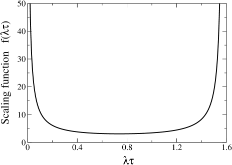
Figure 1: The scaling function $f(\Lambda)\equiv\langle\tilde{h}^{2}(\infty)\rangle/D\tau=\Lambda^{-1}+{{4}\over{\pi}}({{\pi}\over{2}}-\Lambda)^{-1}+1-{{8}\over{\pi^{2}}}$ in the synchronizable regime $0<\Lambda<\pi/2$. Compare this figure with the numerically constructed function presented in Fig. 2 of HKS .

From Eqs. (18) and (22) one learns that for a single stochastic variable governed by Eq. (6) with a nonzero delay, there is an optimal value of the relaxation coefficient $\lambda^{*}={{\pi^{3/2}}/{2(\sqrt{\pi}+2)}}\tau$, at which point the steady-state fluctuations attain their minimum value $\langle\tilde{h}^{2}(\infty)\rangle_{\text{min}}=D\tau(1+2\pi^{-1}+8\pi^{-3/2})$ Note2 , see also HKS .

Returning to the context of network synchronization, one can calculate from Eqs. (5), (12) and (21) the steady-state width of the network-coupled system:

$$\langle w^{2}(\infty)\rangle={{D\tau}\over{N}}\sum_{k=1}^{N-1}\Big{[}{{1}\over{\lambda_{k}\tau}}+{{4}\over{\pi({{\pi}\over{2}}-\lambda_{k}\tau)}}+1-{{8}\over{\pi^{2}}}\Big{]}\ .$$ (23)

Thus, for large $N$ the fundamental limit of synchronization efficiency is given by [see Eq. (22)]:

$$\langle w^{2}(\infty)\rangle_{\text{min}}=D\tau(1+2\pi^{-1}+8\pi^{-3/2})\ .$$ (24)

This is the minimum attainable width of the synchronization landscape in a noisy environment with uniform time delays.

So far we have studied the characteristics of the synchronization network in the steady state ($t\to\infty$) regime. Another interesting characteristic of the synchronization problem is the relaxation time of the network, the time it takes for the system to relax to its finite steady-state width (in the synchronizable regime, $0<\lambda\tau<\pi/2$). As we shall now show, this relaxation time diverges in the $\lambda\tau\to\pi/2$ limit, where the system undergoes a phase transition from a synchronizable state to an unsynchronizable state.

Taking cognizance of Eq. (9), one realizes that the relaxation phase of the network (into a steady state behavior) is governed by the solution of the characteristic equation (11) with the largest real part [Since $\Re(\alpha)<0$ in the synchronizable regime, this amounts to the solution of Eq. (11) with the smallest absolute value of the real part.] Inspection of Eq. (9) reveals that the characteristic relaxation time, $T(\lambda,\tau)$ Note3 , is given by

$$T\equiv{{\tau}\over{2\text{min}\{|\Re(z_{\alpha})|\}}}\ .$$ (25)

Taking cognizance of Eq. (14), one finds

$$T_{\Delta}=\tau{{1+({{\pi}\over{2}})^{2}}\over{\pi\Delta}}\ ,$$ (26)

for the diverging relaxation time of the coupled network in the vicinity of the phase transition (the $\Delta\to 0$ regime).

Further, inserting the pair of solutions $\{z_{+},z_{-}\}$ from (14) into (9), one obtains the late-time behavior of the network near the phase transition:

$$\langle\tilde{h}^{2}(t)\rangle\simeq\langle\tilde{h}^{2}(\infty)\rangle-{{4D\tau}\over{\pi\Delta}}e^{-t/T_{\Delta}}\Big{\{}1+{{\Delta}\over{[1+({{\pi}\over{2}})^{2}]^{2}}}$$

$$\times\Big{[}[({{\pi}\over{2}})^{2}-1]\sin({{\pi t}/{\tau}})+\pi\cos({{\pi t}/{\tau}})\Big{]}\Big{\}}\ .$$ (27)

We thus find that the approach of the network to a steady-state behavior is characterized by damped temporal oscillations of period $2\tau$ and a characteristic lifetime $T_{\Delta}$. It is worth noting that these characteristic oscillations are clearly visible in the numerical results of Hunt et al. HKS (see Fig. 1 of HKS . Observe, in particular, the temporal oscillations in the plots for $\lambda\tau=1.5$ and $\lambda\tau=1.6$ which are near the threshold value $\lambda\tau=\pi/2$ of the phase transition Note4 ).

In summary, in this Letter we have analyzed the problem of network synchronization in a noisy environment with uniform time delays HKS . In particular, we have determined analytically the fundamental limit of synchronization efficiency (the minimum attainable value of the width of the synchronization landscape): $\langle w^{2}(\infty)\rangle_{\text{min}}=D\tau(1+2\pi^{-1}+8\pi^{-3/2})$, where $\tau$ is the characteristic time delay in the communication between pairs of nodes. We have shown that the optimal efficiency of the network is achieved for $\lambda\tau={{\pi^{3/2}}\over{2\sqrt{\pi}+4}}$, where $\lambda$ is the relaxation coefficient (coupling strength). These analytical results are in perfect agreement with the recent numerical results of Ref. HKS . Further, we have analyzed the relaxation time of the network and showed that it diverges in the threshold limit $\lambda\tau\to\pi/2$.

Our results provide a direct analytical explanation for the intriguing trade-off phenomena (between the time delay $\tau$ and the coupling strength $\lambda$) observed in recent numerical simulations HKS of stochastic synchronization problems with time delays.

ACKNOWLEDGMENTS

This research is supported by the Meltzer Science Foundation. I thank Oded Hod, Yael Oren and Arbel M. Ongo for helpful discussions.

References

- (1) A. Arenas et al., Phys. Rep. 469, 93 (2008).
- (2) D. Hunt, G. Korniss and B. K. Szymanski, Phys. Rev. Lett. 105, 068701 (2010).
- (3) G. Korniss, Phys. Rev. E 75, 051121 (2007).
- (4) G. Korniss et al., Science 299, 677 (2003).
- (5) M. Barahona and L. M. Pecora, Phys. Rev. Lett. 89, 054101 (2002).
- (6) T. Nishikawa et al., Phys. Rev. Lett. 91, 014101 (2003).
- (7) F. M. Atay, Phys. Rev. Lett. 91, 094101 (2003).
- (8) C. E. La Rocca, L. A. Braunstein, and P. A. Macri, Phys. Rev. E 80, 026111 (2009).
- (9) C. Zhou, A. E. Motter, and J. Kurths, Phys. Rev. Lett. 96, 034101 (2006).
- (10) T. Nishikawa and A. E. Motter, Phys. Rev. E 73, 065106 (R) (2006).
- (11) R. Olfati-Saber and R. M. Murray, IEEE Trans. Autom. Control 49, 1520 (2004).
- (12) S. Hod and E. Nakar, Phys. Rev. Lett. 88, 238702 (2002).
- (13) S. Hod, Phys. Rev. Lett. 90, 128701 (2003).
- (14) R. Frisch and H. Holme, Econometrica 3, 225 (1935)
- (15) N. D. Hayes, J. Lond. Math. Soc. s1-25, 226 (1950).
- (16) Synchronizability of the entire network requires a finite steady-state width, . Thus, the synchronizability condition is given by for all modes HKS .
- (17) This finding is in stark contrast to the case of coupled networks without time delays, in which case one finds ; i.e., there the steady-state fluctuation is a monotonically decreasing function of the relaxation coefficient HKS .
- (18) It is clear from Eqs. (9) and (11) that , where is a scaling function.
- (19) For , the characteristic oscillations are best seen in the interval . From Fig. 1 of HKS one may confirm that the period of the damped oscillations is indeed .