Transition to miscibility in linearly coupled binary dipolar Bose-Einstein condensates

Abstract

We investigate effects of dipole-dipole (DD) interactions on immiscibility-miscibility transitions (IMTs) in two-component Bose-Einstein condensates (BECs) trapped in the harmonic-oscillator (HO) potential, with the components linearly coupled by a resonant electromagnetic field (accordingly, the components represent two different spin states of the same atom). The problem is studied by means of direct numerical simulations. Different mutual orientations of the dipolar moments in the two components are considered. It is shown that, in the binary BEC formed by dipoles with the same orientation and equal magnitudes, the IMT cannot be induced by the DD interaction alone, being possible only in the presence of the linear coupling between the components, while the miscibility threshold is affected by the DD interactions. However, in the binary condensate with the two dipolar components polarized in opposite directions, the IMT can be induced without any linear coupling. Further, we demonstrate that those miscible and immiscible localized states, formed in the presence of the DD interactions, which are unstable evolve into robust breathers, which tend to keep the original miscibility or immiscibility, respectively. An exception is the case of a very strong DD attraction, when narrow stationary modes are destroyed by the instability. The binary BEC composed of co-polarized dipoles with different magnitudes are briefly considered too.

I Introduction

The development of the trapping techniques has made it possible to create multicomponent Bose-Einstein condensates (BEC) formed by atoms in different electronic states trapp . The multicomponent BEC is an ideal system for studying phase transitions and the coexistence of different phases, which are topics of great significance to many areas of physics. The advantage of the gaseous BEC systems is the possibility to very accurately describe their dynamics in the framework of the mean-field approximation. This approach does not apply to multicomponent quantum systems in condensed states, because their densities are much higher, making the delta-functional pseudopotential, which is used to describe the local interactions between atoms in dilute BEC  by means of the single scattering-length parameter, inappropriate.

In particular, experiments have been performed in a binary BEC created in ⁸⁷Rb, which contains atoms in two different hyperfine (spin) states trapp . The physics of binary BECs gives rise to novel paradigms for ground-states wave function and excitations on top of them ground , binaryinol . One generic scenario concerning the binary condensates leads to an equilibrium state characterized by separation of two immiscible species in different spatial domains domain . In addition, a resonant electromagnetic spin-flipping field, with a frequency in the range of several GHz, can induce a linear coupling (interconversion) between the two species treca . This technique opens a way to observe various effects, such as Josephson oscillations between the two states peta , domain walls sesta , “co-breathing” oscillation modes sedma , nontopological vortices osma , and others.

In the absence of the linear coupling between the components, the superfluid components formed by atoms in two hyperfine states of ⁸⁷Rb, $\left|F=1,m_{F}=-1\right\rangle$ and $\left|F=2,m_{F}=+1\right\rangle$, are immiscible, although being close to the miscibility threshold. On the contrary, the mixture of $\left|F=1,m_{F}=1\right\rangle$ and $\left|F=2,m_{F}=2\right\rangle$ states is miscible, but the separation between them can be induced by a gradient of the magnetic field Ketterle , or by causing them to flow in opposite directions Engels . The dynamics of the separation between the two respective superfluid components has been studied in detail experimentally Rb-separation .

The immiscibility-miscibility transition (IMT) in the binary BEC may be induced through the Feshbach resonance, which makes it possible to change the scattering lengths for inter-atomic collisions by means of an external magnetic field deseta , or a properly tuned coherent optical signal jedanaesta . In particular, the change of the miscibility of ⁸⁵Rb and ⁸⁷Rb condensates by means of the Feshbach resonance, which affects the intrinsic scattering length of the former species, was demonstrated in the experiments 85-87 .

On the other hand, it has also been shown that the IMT between the components which represent different spin states of the same atom may be induced by the linear coupling between them glavna . In this way, an immiscible binary condensate may be converted into a miscible one, using the spin-flipping electromagnetic wave of a rather small amplitude.

In all the above-mentioned cases, the studies of the binary condensates were limited to the case of contact inter-particle interactions. On the other hand, a great deal of attention has been recently drawn to dipolar BECs. They can be created in gases of ultracold polar molecules ultra , in chromium chrom , or in the case when atomic electric dipoles are induced by the optical pumping of atoms into a Rydberg state. Binary dipolar BECs are possible too – in particular, those formed by atoms in two different Rydberg states rydberg . Another realization of a dipolar mixture is possible in condensates of heteronuclear diatomic molecules classified as type A according to the Hund’s nomenclature Hund , in which the direction of the magnetic moment is correlated (parallel or antiparallel) with the orientation of the molecular axis goral . Through this mechanism, a binary BEC with antiparallel dipolar components can be created. As shown in Ref. goral and in this paper (see below), binary mixtures of the latter type may feature remarkable properties.

The goal of this paper is to analyze the IMT in the binary dipolar BEC formed by the same atoms in different hyperfine states, in the presence of the linear coupling between the components. It may be expected that the nonlocal character of the dipole-dipole (DD) interactions may essentially affect the spatial separation between the components in the binary condensate. In accordance with this, the main issues we are addressing here are effects of the DD interactions on the IMT, including a possibility to induce the IMT by the DD interactions without the linear interconversion between the constituents.

The paper is structured as follows. In section II, equations describing the two-component dipolar BEC in the harmonic trap, including the linear coupling between the components, are introduced. This is a system of one-dimensional (1D) integro-differential equations, with the nonlocal DD interaction terms set down as in Ref. goral . Section III presents basic results obtained for the binary dipolar mixtures, with different combinations of orientations and magnitudes of the dipole moments in the two components. The effect of the DD interactions on the IMT is studied numerically, for a fixed total number of atoms, $N_{1}+N_{2}=\mathrm{const}$. Dynamical properties of localized mixed and separated states are considered too. The paper is concluded by section IV.

II The model

The quasi-1D dynamical equations for the dipolar BEC trapped in the harmonic-oscillator (HO) potential are derived starting from the rescaled Gross-Pitaevskii equation (GPE) with the short-range and DD interactions,

$$i\frac{\partial}{\partial t}\Psi(\vec{r},t)=\left[-\frac{1}{2}\nabla^{2}+\frac{1}{2}(\omega_{\rho}^{2}\rho^{2}+\omega_{z}^{2}z^{2})+\gamma|\Psi(\vec{r},t)|^{2}+G\int d\vec{r^{\prime}}\frac{1-3\cos^{2}\theta}{\left|\vec{r}-\vec{r^{\prime}}\right|^{3}}|\Psi(\vec{r^{\prime}},t)|^{2}\right]\Psi(\vec{r},t),$$ (1)

following Ref. lsantos . In Eq. (1), wave function $\Psi(\vec{r},t)$ is normalized to the total number of atoms, $\omega_{\rho}$ and $\omega_{z}$ are normalized trapping frequencies in the transverse and axial ($z$) direction, $\rho\equiv\sqrt{x^{2}+y^{2}}$, $\theta$ is the angle between the parallel dipoles and vector $\left(\vec{r}-\vec{r^{\prime}}\right)$, and coefficients $\gamma$ and $G$ measure, respectively, the strengths of the contact and DD interactions. The only assumption in the subsequent derivation is the standard single-mode approximation for the transversal part of the wave function, i.e., it is substituted by $\Psi(z,\rho,t)=\psi(z,t)\phi_{0}(\rho)$, where $\phi_{0}(\rho)=(\sqrt{\pi}l)^{-1}\exp(-\rho^{2}/2l^{2})$, and $l=1/\sqrt{\omega_{\rho}}$ is the characteristic harmonic-oscillator length which determines the transverse localization. The averaging in the transverse plane leads to an effective 1D kernel of the DD interaction lsantos ,

$$V_{\mathrm{DD}}(z)=\frac{2\alpha G}{l^{3}}\left[2\sqrt{\tau}-\sqrt{\pi}(1+2\tau)\exp{(\tau)}\mathrm{erfc}(\sqrt{\tau})\right],$$ (2)

where $\tau\equiv(z/l)^{2}$, $\alpha=1\,$and $\alpha=-0.5$ for $\theta=0$ and $\theta=\pi/2$, i.e., respectively, for the polarization of the dipoles along and perpendicular to axis $z$, and $\mathrm{erfc}$ is the complementary error function. Being interested in effects of the DD interactions on the IMT in binary BEC, we will focus on the basic situation, when the characteristic axial length scale is much larger than the transverse size, $Z\gg l$. In particular, the experimental setting with aspect ratio $Z/l\simeq 10$ was realized in the chromium condensates experim1 ; review . Under this condition, expression (2) yields results which are practically tantamount to those obtained with the use of the standard form of the DD interaction kernel, $V_{DD}\sim 1/|z|^{3}$, truncated on the scale of $z\sim l$ (the analysis performed in Ref. Cuevas for gap solitons in the quasi-1D condensate including the DD repulsion or attraction and a periodic potential, has demonstrated that the difference in the results generated by means of the different kernels is limited to $\lesssim 3\%$). Therefore in the numerical calculations the DD interaction kernel was taken in the usual regularized (truncated) form.

Proceeding to the consideration of the effectively 1D two-component trapped BEC, we use a system of nonlinearly coupled GPEs, which include the DD terms, for the wave functions of the two components, $\psi_{1}(z,t)$ and $\psi_{2}(z,t)$. If they represent different hyperfine states of the same atom, the interconversion, induced by a resonant electromagnetic wave, is accounted for by linear mixing terms ist ; bitanstabrad . The scaled form of the respective GPE system is

$$i\frac{\partial\psi_{1}}{\partial t}=-\frac{1}{2}\frac{\partial^{2}\psi_{1}}{\partial z^{2}}+V_{0}z^{2}\psi_{1}+(\gamma_{11}|\psi_{1}|^{2}+\gamma_{12}|\psi_{2}|^{2})\psi_{1}-\kappa\psi_{2}+$$

$$+\psi_{1}\left(G_{11}\int_{-\infty}^{+\infty}\,dz^{\prime}\frac{|\psi_{1}(z^{\prime})|^{2}}{|z-z^{\prime}|^{3}}+G_{12}\int_{-\infty}^{+\infty}\,dz^{\prime}\frac{|\psi_{2}(z^{\prime})|^{2}}{|z-z^{\prime}|^{3}}\right),$$

$$i\frac{\partial\psi_{2}}{\partial t}=-\frac{1}{2}\frac{\partial^{2}\psi_{2}}{\partial z^{2}}+V_{0}z^{2}\psi_{2}+(\gamma_{21}|\psi_{1}|^{2}+\gamma_{22}|\psi_{2}|^{2})\psi_{2}-\kappa\psi_{1}+$$

$$+\Delta\mu\cdot\psi_{2}+\psi_{2}\left(G_{21}\int_{-\infty}^{+\infty}\,dz^{\prime}\frac{|\psi_{1}(z^{\prime})|^{2}}{|z-z^{\prime}|^{3}}+G_{22}\int_{-\infty}^{+\infty}\,dz^{\prime}\frac{|\psi_{2}(z^{\prime})|^{2}}{|z-z^{\prime}|^{3}}\right),$$ (3)

where $V_{0}$ is the strength of the axial trap, $\gamma_{11}$, $\gamma_{22}$ and $\gamma_{12}$, $\gamma_{21}$ are, respectively, the coefficients accounting for intra-species and inter-species contact interaction, $\kappa$ is the linear coupling, and $\Delta\mu$ is a possible chemical-potential difference between the two components, which may be induced by an external dc magnetic field interacting with the atomic spins. Further, the DD interaction coefficients, $G_{11},G_{12},G_{21},G_{22}$, are defined as

$$\left\{G_{11},G_{12},G_{21}G_{22}\right\} = \left\{\nu\mu_{1}^{2},(1-\nu)\mu_{1}\mu_{2},\nu\mu_{1}\mu_{2},\left(1-\nu\right)\mu_{2}^{2}\right\}$$ (4)

$$\times\left(\mu_{0}/4\pi\right)(1-3\cos^{2}{\theta}),$$

where $\mu_{0}$ is the magnetic permeability of vacuum, $\mu_{1},\,\mu_{2}$ are the dipole moments in two BEC components, $\nu\equiv N_{1}/N$ denotes the ratio of the atom numbers in them, and $N=N_{1}+N_{2}$ is the total number of atoms. The angle between the system’s axis and the dipole orientations is $\theta$, as before. Below, we focus on the two above-mentioned basic orientations: parallel ($\theta=0$) and perpendicular ($\theta=\pi/2$), which correspond, respectively to the attractive and repulsive DD interactions. Two dynamical invariants of Eqs. (3) are the total norm,

$$P=\int_{-\infty}^{+\infty}dz\,\left(|\psi_{1}|^{2}+|\psi_{2}|^{2}\right),$$ (5)

and energy (Hamiltonian)

$$E = E_{0}+E_{\mathrm{coupl}}+E_{\mathrm{DD}}~{},$$

$$E_{0} = \int_{-\infty}^{+\infty}dz\,\left[-\frac{1}{2}\left(|\partial\psi_{1}/\partial z|^{2}+|\partial\psi_{2}/\partial z|^{2}\right)+V_{0}z^{2}\left(|\psi_{1}|^{2}+|\psi_{2}|^{2}\right)\right]$$

$$+ \int_{-\infty}^{+\infty}dz\,\left[\frac{1}{2}\left(\gamma_{11}|\psi_{1}|^{4}+\gamma_{22}|\psi_{2}|^{2}\right)+\gamma_{12}|\psi_{1}|^{2}|\psi_{2}|^{2}\right],$$

$$E_{\mathrm{coupl}} = -\int_{-\infty}^{+\infty}dz\,\left(\kappa(\psi_{1}\psi_{2}^{\ast}+\psi_{1}^{\ast}\psi_{2})-\Delta\mu|\psi_{2}|^{2}\right),$$

$$E_{\mathrm{DD}} = \int_{-\infty}^{+\infty}dz\,\left[\left(G_{11}|\psi_{1}|^{2}+G_{21}|\psi_{2}|^{2}\right)\int_{-\infty}^{+\infty}dz^{\prime}\,\frac{|\psi_{1}(z^{\prime})|^{2}}{|z-z^{\prime}|^{3}}\right]+$$ (6)

$$+ \int_{-\infty}^{+\infty}dz\,\left[(G_{12}|\psi_{1}|^{2}+G_{22}|\psi_{2}|^{2})\int_{-\infty}^{+\infty}dz^{\prime}\,\frac{|\psi_{2}(z^{\prime})|^{2}}{|z-z^{\prime}|^{3}}\right].$$

Stationary solutions are looked for as $\psi_{1,2}(z,t)=\phi_{1,2}(z)\exp{(-i\mu\,t)}$, where $\mu$ is the chemical potential (in the presence of the linear coupling, the chemical potential of both components must be the same glavna ), and real functions obey the following integro-differential equations:

$$\mu\phi_{1} = -\frac{1}{2}\frac{d^{2}\phi_{1}}{dz^{2}}+V_{0}z^{2}\phi_{1}+(\gamma_{11}|\phi_{1}|^{2}+\gamma_{12}|\phi_{2}|^{2})\phi_{1}-\kappa\phi_{2}+$$

$$+ \phi_{1}\left(G_{11}\int_{-\infty}^{+\infty}\,dz^{\prime}\frac{|\phi_{1}(z^{\prime})|^{2}}{|z-z^{\prime}|^{3}}+G_{12}\int_{-\infty}^{+\infty}\,dz^{\prime}\frac{|\phi_{2}(z^{\prime})|^{2}}{|z-z^{\prime}|^{3}}\right)$$

$$\mu\phi_{2} = -\frac{1}{2}\frac{d^{2}\phi_{2}}{dz^{2}}+V_{0}z^{2}\phi_{2}+(\gamma_{21}|\phi_{1}|^{2}+\gamma_{22}|\phi_{2}|^{2})\phi_{2}-\kappa\phi_{1}+$$ (7)

$$+ \phi_{2}\left(G_{21}\int_{-\infty}^{+\infty}\,dz^{\prime}\frac{|\phi_{1}(z^{\prime})|^{2}}{|z-z^{\prime}|^{3}}+G_{22}\int_{-\infty}^{+\infty}\,dz^{\prime}\frac{|\phi_{2}(z^{\prime})|^{2}}{|z-z^{\prime}|^{3}}\right)+\Delta\mu\cdot\phi_{2}.$$

Properties of the binary BEC described by this model depend on a large number of parameters, including the number of particles in each component and the magnitudes and orientations of the dipoles. In the following, the results are presented for $\gamma_{11}=\gamma_{22}=10,\,\gamma_{12}=\gamma_{21}=20,\,\Delta\mu=0,\,V_{0}=0.5$, and equal numbers of atoms in both components, i.e., $\nu=0.5$. As for the DD terms, we assume that the dipole moments of the two components are oriented in the same direction, with all the DD strengths being equal, $G_{11}=G_{22}=G_{12}=G_{21}\equiv\Gamma$ (case I), or with different strengths, $G_{11}=\Gamma,\,G_{12}=G_{21}=1.1\Gamma$, and $G_{22}=1.21\Gamma$ (case II). As seen from Eqs. (4), cases I and II correspond, respectively, to equal magnitudes of the dipole moments, $\mu_{1}=\mu_{2}$, and unequal ones, $\mu_{2}=1.1\mu_{1}$. The case of the BEC composed of two identical components polarized in opposite directions, $G_{11}=G_{22}=-G_{12}=-G_{21}=\Gamma$ (case III) is considered too. The latter one corresponds to the above-mentioned setting composed of type-A molecules, in terms of the Hund nomenclature, under the action of the magnetic field, which determines the orientation of the magnetic moments, while the electric dipolar moments can be parallel or antiparallel to the direction of the applied magnetic field goral .

In the absence of the DD interactions and linear coupling, Eqs. (3) or (7) can be solved, under specific conditions, analytically by means the inverse scattering technique ist , and numerically in the general case numoutdd . In particular, both the analytical and numerical solutions produce solitons. On the other hand, the localized miscible and immiscible states were found in the condensate with two components coupled by the linear interconversion. The IMT in the binary condensate can be controlled by the strength of the linear driving glavna . The critical value of the linear-coupling parameter for the IMT was estimated, by means of the variational approximation, to be $\kappa_{\mathrm{cr}}=(\gamma_{12}-\gamma_{11})/2$, which has been confirmed by the numerical simulations. In this work, we use numerical methods to find fundamental solutions of Eq. (3) for the binary dipolar BEC, and explore effects of the DD interactions on the IMT in this system.

III Immiscibility-miscibility transitions

In this section, we present results corresponding to the fixed norm (rescaled number of atoms), $P\approx 4$, a free parameter being the linear coupling, $\kappa$. As mentioned above, the parameters of contact interactions and trapping potential are the same as in Ref. glavna : $\gamma_{11}=\gamma_{22}=\gamma_{12}/2=\gamma_{21}/2=10$ and $V_{0}=0.5$, which correspond to the strong immiscibility, in the absence of the linear coupling and DD interactions. This may be realized so that the two species do not mix because their mutual repulsion is stronger than the intrinsic repulsion between atoms belonging to the same species.

As concerns the parameters of the DD interactions, we will consider the following characteristic cases, I, II, and III (as mentioned above): $G_{11}=G_{12}=G_{21}=G_{22}\equiv\Gamma$, or $G_{11}\equiv\Gamma,\,G_{12}=G_{21}=1.1\Gamma,\,G_{22}=1.21\Gamma$, or $G_{11}=-G_{12}=-G_{21}=G_{22}\equiv\Gamma$. Recall that $\Gamma<0$ and $\Gamma>0$ correspond to the attractive and repulsive DD interactions, respectively. Stationary states were obtained by simulations of Eqs. (3) in imaginary time. In the absence of the DD interactions, slightly perturbed stationary states maintain themselves (in real time) as breathing localized modes with the conserved norm glavna .

III.0.1 Equal dipole moments in both components

In the absence of the linear coupling between the components, or with a very weak linear coupling, the addition of the arbitrary strong repulsive DD interaction to an initially immiscible state of the binary system cannot induce a transition to miscibility, see Fig. 1(a). However, the increase of the repulsive DD-interaction strength in the presence of a somewhat stronger linear coupling, which still corresponds to the immiscible phase in the case with only contact interaction, $\kappa<\kappa_{\mathrm{cr}}$ (see Ref. glavna ), can stimulate the IMT, as shown in 1(b). In the presence of the repulsive DD interactions, the miscible state generated by the linear interconversion remains miscible, but the nonlocal interaction makes the amplitude of the trapped mixed state smaller, and its width larger, as seen in Fig. 1(c). These results may be summarized by stating that the repulsive DD interaction tends to mix the separated components, but it can do this only in the combination with the linear interconversion between them, while the interplay of the DD repulsion with the contact nonlinear interactions is less important, in terms of the qualitative description.

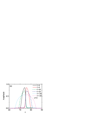
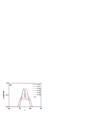
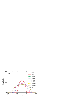
Figure 1: (Color online) The amplitude profiles of stationary states in the binary BEC for different values of the linear-coupling constant: (a) $\kappa=0.1$, (b) $\kappa=2$, and (c) $\kappa=3$. In each case, the profiles are displayed for the varying strength of the repulsive DD interaction, $G_{11}=G_{22}=G_{21}=G_{12}\equiv\Gamma$. In this and other figures, parameters $\gamma_{mn}\$($m,n=1,2$), which characterize the contact repulsion, are $2\gamma_{11}=2\gamma_{22}=\gamma_{12}=\gamma_{21}=20$.

The stability of the localized states was checked by direct simulations of their perturbed evolution in the real time. It was found that both the miscible and immiscible states are stable, although the former ones are more sensitive to asymmetric perturbations than their immiscible counterparts with the same norm. Generally, the perturbations give rise to small persistent intrinsic vibrations in the trapped states (not shown here).

In the presence of the attractive DD interaction, the components that were separated at $\kappa=0.1$, in the absence of the DD interactions, remain separated. Naturally, with the increase of the DD attraction strength, the localized states become narrower and taller, see Fig. 2. However, localized states cannot be found for an arbitrarily large strength of the DD attraction (an explanation to this fact is given below). In other words, there is an upper limit of the strength, beyond which the attractive DD forces cannot support localized modes. The latter conclusion is consistent with the real-time simulations, which confirm that the BEC components stay separated, unless the DD attraction is so strong that it destroys both components. An example of the evolution of the initially separated state in the presence of the strong attractive DD interaction, but yet below the destruction threshold, is shown in Fig. 3 for $\Gamma=-10$. Although the central part of the mode stays localized, the mode radiates a significant part of its norm.

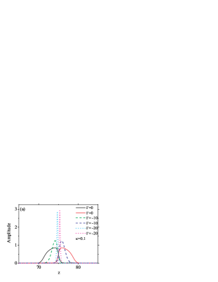
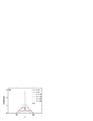
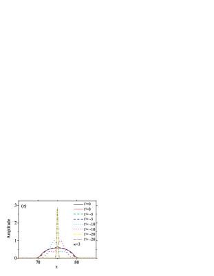
Figure 2: (Color online) The amplitude profiles of stationary states of the binary BEC for different values of $\kappa$: (a) $\kappa=0.1$, (b) $\kappa=2$, and (c) $\kappa=3$, in the presence of the attractive DD interaction with $\Gamma\equiv G_{11}=G_{22}=G_{21}=G_{12}$. The values of $\Gamma<0$ are indicated in the plots.

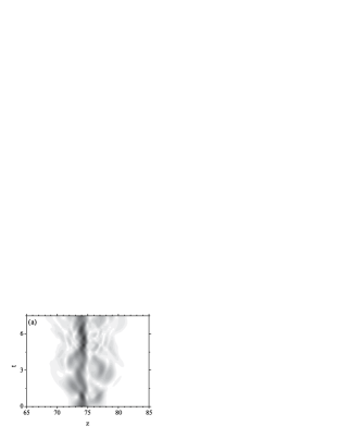
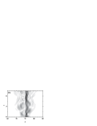
Figure 3: (Color online) The amplitude profiles versus time for a slightly perturbed immiscible state with $\kappa=2,\,\Gamma=-10$. Panels (a) and (b) display the evolution of the two components. The initial (dotted and dotted-dashed) profile and the one at $t=7.5$ (solid and dashed curves) are shown in (c).

In the parameter region near the IMT induced by the linear coupling in the absence of the DD interactions [for example, at $\kappa=2$, see Fig. 2(b)], the increase of the strength of the attractive DD interaction again makes the immiscible localized mode narrower and taller. Very strong DD attraction may result in a miscible state with a very high amplitude and very narrow shape. However, such states are unstable and disintegrate with time. An example of the instability is displayed in Fig. 4.

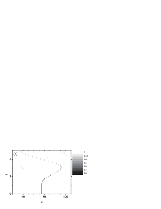
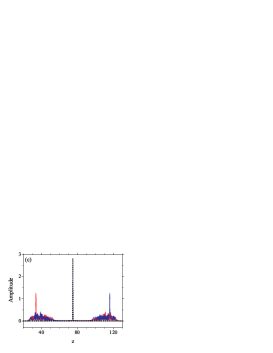
Figure 4: (Color online) The amplitude profiles versus time for a slightly perturbed mixed state with $\kappa=2,\,\Gamma=-20.$Panels (a) and (b) show the evolution of the two components. The initial very narrow profile (dotted black curves) and the one at $t=7.5$ (continuous blue and red curves) are plotted in (c).

In the region of $\kappa$ slightly above $\kappa_{\mathrm{cr}}$, i.e., in the states which are miscible in the absence of  the DD interactions, the presence of the weak DD attraction may lead to a transition back to the immiscible state, which is unstable. In the rest of the region with $\kappa>\kappa_{\mathrm{cr}}$, the increase of the attractive DD interaction leads to taller and narrower miscible localized states, see Fig. 2 (c). These newly formed miscible states are also unstable to small perturbations. Localized states cannot be formed if the DD attraction is too strong, similar to what was said above for smaller $\kappa$.

The nonexistence of localized states in binary BEC for arbitrary values of $\kappa$ in the presence of very strong attractive DD interactions is a consequence of the singularity in the 1D condensate model, which manifests itself when the characteristic length of the DD interaction becomes comparable to the inter-particle distance goral . This is related to the singularity in the single-component BEC, in the case when the negative pressure caused by the inter-particle attraction is not compensated by the quantum pressure in the trapping potential rydberg , goral .

Thus, the DD interactions can effect the IMT in the dipolar BEC mixture, with the components polarized in the same direction (and with equal magnitudes of the magnetic moments), which are coupled by the linear interconversion. This is a direct consequence of the nonlocality of the DD interactions. However, the DD interactions of either sign (repulsive or attractive), by themselves, cannot induce the IMT, as seen in Fig. 5(a). On the other hand, the repulsive and attractive DD interactions’ shift of the equilibrium in favor of the miscibility and immiscibility, respectively.

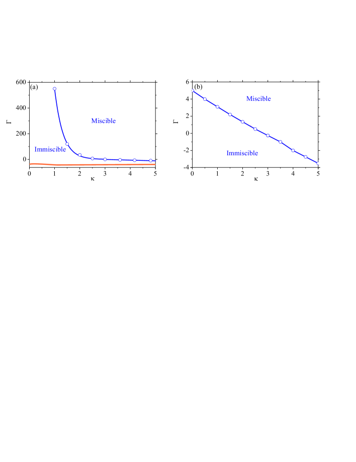
Figure 5: (Color online) The blue lines with circles show the immiscibility-miscibility transition curves in the parameter space, ($\Gamma$,  $\kappa$), produced by the numerical calculations for cases I (co-polarized components, panel a) and III (counter-polarized components, panel b). The areas of miscible and immiscible states (above and below the transition lines with symbols) are labeled accordingly. Below the red thick line, localized states in the binary BEC with co-polarized dipolar components (case I) were not found.

A transition to the miscibility may be induced by the DD interactions (in the absence the linear interconversion) if the two dipolar components are polarized in the opposite directions, which was defined above as case III, with $\mu_{1}=-\mu_{2}$ in Eqs. (4). Recall that such a situation can be realized for molecules of the Hund’s type A in the external magnetic field goral . The possibility to induce the IMT by the DD interaction in this case is illustrated by Fig. 6 (a), which corresponds to the model without the linear coupling.

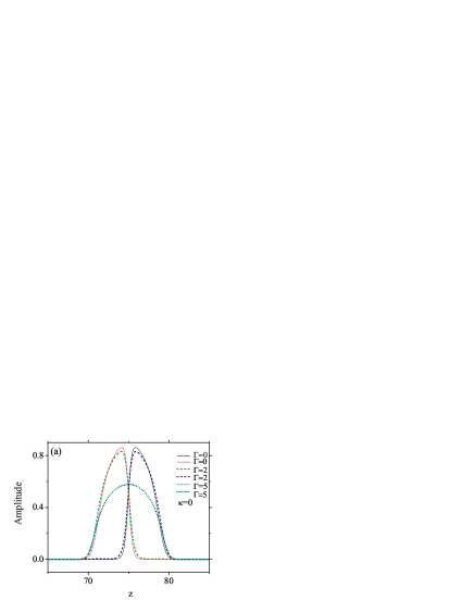
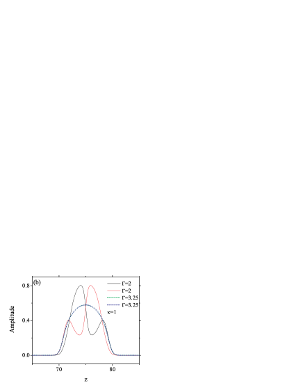
Figure 6: (Color online) Amplitude profiles of stationary states for the two-component dipolar mixture with counter-polarized components: (a) in the absence of the linear coupling ($\kappa=0$) and (b) for $\kappa=1$. Parameters of the DD interaction are $G_{11}=G_{22}=\Gamma,\,G_{21}=G_{12}=-\Gamma$, with values of $\Gamma$ indicated in the plot. The transition to the miscibility with the increase of $\Gamma$ is evident.

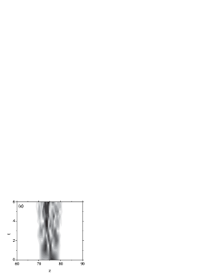
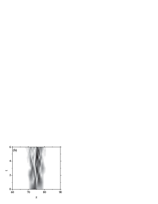
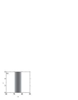
Figure 7: 2D plots of the evolution in case III (counter-polarized components) with $\kappa=1$: (a) and (b) the evolution of the two components initialized in the immiscible state for $\Gamma=2$; (c) the evolution of a stable miscible state for $\Gamma=3.25$, cf. Fig. 6(b). The immiscible states evolve as localized structures with complex intrinsic patterns, while the miscible state evolves as a regular breather.

The numerically found IMT curve for case III (the counter-polarized components) in the parameter space of ($\Gamma$, $\kappa$) is displayed in Fig. 5(b). In this case, the addition of the linear interconversion shifts the transition to the miscibility to a lower strength of the DD interaction. Figure 7 displays examples of the evolution of immiscible and miscible states for $\kappa=1$ which are presented in Fig. 6(b). The immiscible state evolves as a localized mode with a complex intrinsic structure, while the miscible state is only slightly perturbed, evolving into a regular breather. Note that, in case III, with the opposite polarizations of the dipoles in the two components, i.e., $G_{11}=G_{22}=\Gamma<0,\,G_{12}=G_{21}=\Gamma>0$, the IMT to a stable miscible state cannot be induced by the DD interactions in the absence of the linear interconversion, see Fig. 5 (b). In this case, only a narrow strongly pinned miscible state is formed, which is unstable.

In fact, the configuration with the counter-polarized components considered here implies that, in both of them, the moments are directed along the spatial axis. The other case, with the counter-polarized components oriented perpendicular to the axis, is possible too, in which case the DD interaction is attractive between the components and repulsive inside each component.

To summarize the analysis of cases I and III, we have found that the repulsive DD interactions affect the IMT, but only in the presence of the linear coupling in the case I– namely, the curve with circles in Fig. 5(a) shows the critical values of $\kappa$ which are lower than their counterparts found in the absence of the DD interactions. In this case, both the miscible and immiscible stationary modes remain stable under the action of the DD repulsion. The weak attractive DD interactions may convert a miscible state near the IMT threshold ($\kappa\approx\kappa_{\mathrm{cr}}$) into an unstable immiscible one. At larger values of $\kappa>\kappa_{\mathrm{cr}}$, the increase of the attractive DD interaction causes the formation of tightly pinned miscible states, which are strongly unstable. There is a limiting value of the strength of the DD attraction, above which localized states cannot exist in the binary BEC. Finally, for the condensate with counter-polarized components (case III), the numerical results reveal the existence of the single IMT point, $\Gamma$, which moves to smaller values with the increase of $\kappa$, see Fig. 5 (b).

III.0.2 Unequal magnitudes of the dipole moments in the two components

In the model describing binary BEC formed of atoms with equal dipole moments, which was considered above, it is obvious that all the states are spatially symmetric, in terms of the total density of both species (before and after the IMT, and for both the co- and counter-polarized components). On the other hand, in the binary system with different dipole moments of the two species an issue is not only the IMT itself, but also the equilibrium partition of atoms between the species [cf. Ref. glavna , where an asymmetry between the species was introduced through the difference in the chemical potentials, $\Delta\mu$ in Eqs. (3).

Here we present results for slightly different magnitudes of the dipole moments, viz., $G_{11}\equiv\Gamma,G_{22}=1.21\Gamma,G_{21}=G_{12}=1.1\Gamma$, and several different values of $\Gamma$. In the presence of the repulsive DD interactions at small $\kappa$, immiscible states are formed, in which the shapes of the two components may be spatially asymmetric. Depending on the initial profile used in the imaginary-time simulations, which were taken as two Gaussians with coinciding or separated centers, two distinct types of stationary immiscible states could be found, respectively, in the binary system: those which feature the mirror symmetry between $\phi_{1}(z)$ and $\phi_{2}(z)$, and asymmetric ones, see Fig. 8. Computing energies of the observed states, we have found that the energy is smaller (by a few per cent) in the asymmetric state. Nevertheless, it does not represent the ground state of the system, because in direct simulations this stationary state develops into a breather, as shown in Fig. 8. Note that the component with the larger dipole moment features a smaller amplitude. Opposite to the case of equal dipole moments, where the growth of the repulsive DD interaction could lead to the IMT at $\kappa\neq 0$, here the growth of the DD repulsion increases the separation between the components. A noteworthy difference of the immiscible states in the present case from their counterparts in the model with equal dipole moments (cf. Figs. 1, 2, 3 for the case of the co-polarized components, and Fig. 6 for the counter-polarization) is that the unequal moments give rise to three-lobe shapes. They feature two regions occupied by the component with the larger dipole moment, which are separated by a single region in which the component with the smaller moment is concentrated.

The character of the mixed states generated due to the linear coupling is not changed in the presence of the repulsive DD (of course, the shapes of the two components become different). Real-time simulations indicate that the immiscible and miscible localized states in the binary system with different dipole moments of the components evolve into breathing structures, which tend to keep the original immiscible or miscible structure of the pattern. This is the case for both symmetric and asymmetric profiles of the two components, which is understandable due to very close energies of the immiscible and miscible modes (the energy difference between them is $\lesssim 1\%$). An example of the breather developing from immiscible modes is displayed in Figs. 8(c,d).

The attractive DD interaction pushes all binary states in the system with unequal dipole moments to enhanced immiscibility, see Fig. 9 (which is consistent with effects of the DD attraction outlined above in the symmetric system). As well as in the case of the DD repulsion, the symmetry of the stationary states obtained from the imaginary-time simulations depends on the initialization, cf. Figs. 8 and 10(a),(b). The separated asymmetric states are getting more and more asymmetric and both symmetric and asymmetric ones are becoming more and more narrow with the growth of $|\Gamma|$. The maximum energy difference between the symmetric and asymmetric states for fixed $\Gamma$ is of the order of a few per cents. The stationary mixed state which exists without the DD interaction for certain values of $\kappa$ is transformed by the DD attraction into immiscible states whose symmetry is determined by the initial conditions, see Fig. 10(b). Note that, in the case of the DD attraction, the stationary localized states can only be found if the DD interaction strength is not too large. Real-time simulations demonstrate that all localized states which exist in the presence of the attractive DD interaction are unstable, see Figs. 10 (c)-(f).

The results presented above, and additional ones not displayed here, that were obtained for different combinations of the DD interaction parameters, show a great diversity of possible localized states in binary BEC with components formed of atom with different moments. Generally, their symmetry properties, shape, and width depend on the initial conditions.

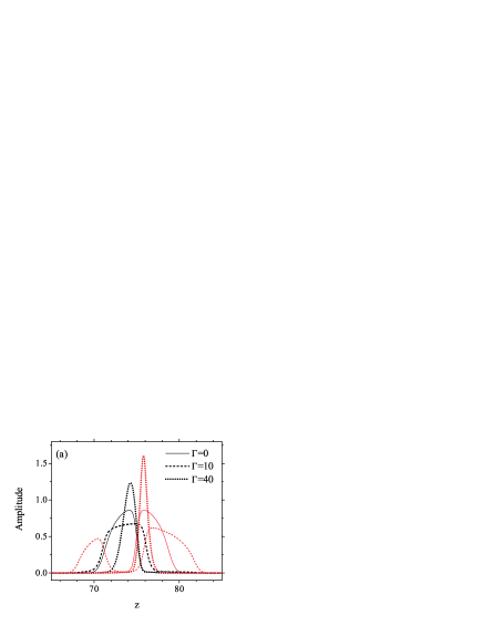
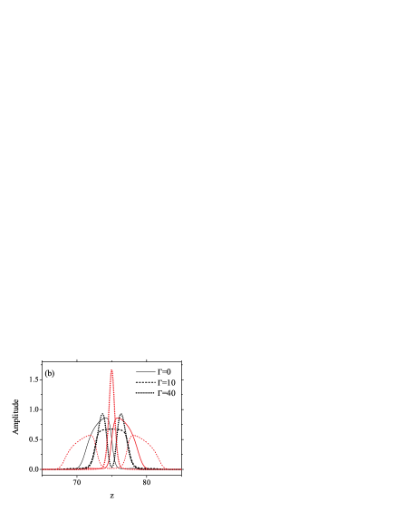
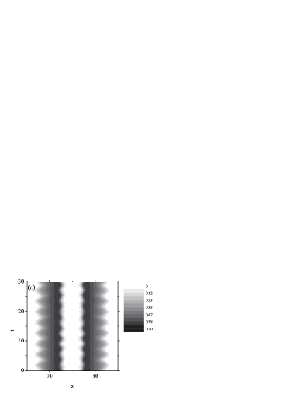
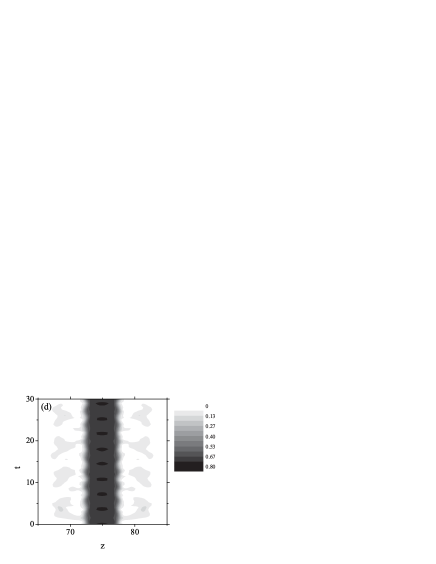
Figure 8: (Color online) Profiles of the trapped modes in the binary BEC with $\kappa=0.1$, produced by the imaginary-time simulations which were initialized by separated (a) or overlapping (b) Gaussians. In the absence of the DD interactions, the corresponding state is immiscible, independently of the initialization. In the presence the DD interaction, the modes evolve into breathers, as plotted for both components in (c) and (d) for $\Gamma=40$ [the respective initial profile is presented by the dashed line in (b)]. Parameters of the DD interactions are $G_{11}=\Gamma=40,\,G_{21}=G_{12}=1.1\Gamma,$ and $G_{22}=1.21\Gamma$.

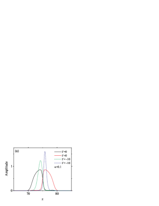
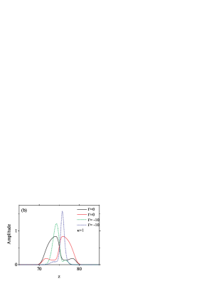
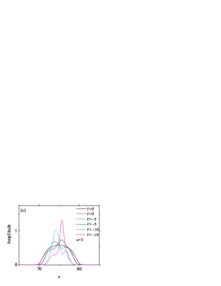
Figure 9: (Color online) Profiles of asymmetric stationary states in the binary BEC for different values of the linear-coupling constant: (a) $\kappa=0.1$, (b) $\kappa=2$, and (c) $\kappa=3$. The strengths of the attractive DD interaction are $G_{11}=\Gamma,G_{22}=1.21\Gamma,$ and $G_{21}=G_{12}=1.1\Gamma$. The respective values of $\Gamma$ are indicated in the plots.

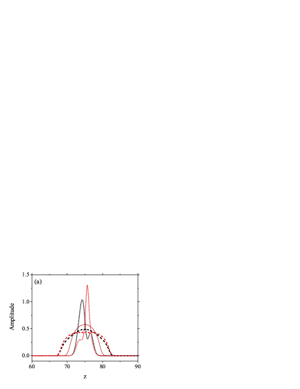
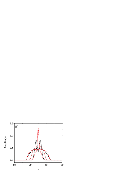
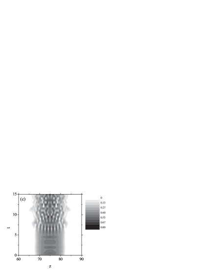
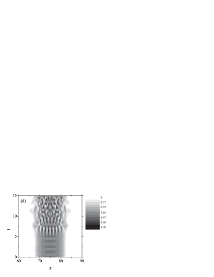
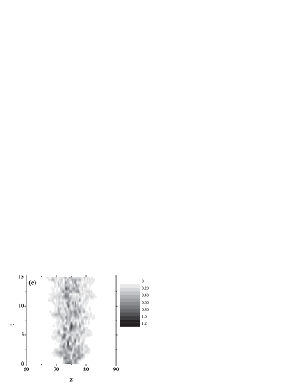
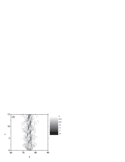
Figure 10: (Color online) Profiles of the localized modes in binary BEC with $\kappa=3$, obtained by means of the imaginary-time simulations with initial conditions in the form of separated (a) and overlapping (b) Gaussians: $\Gamma=0$ (solid lines), $\Gamma=40$ (dashed lines), and $\Gamma=-10$ (dotted lines). In the absence of the DD interaction, the corresponding state is miscible, irrespective of the initialization. The states are unstable for either sign of the DD interaction, as shown in (c), (d) for $\Gamma=40$ [the respective initial profile is shown by the dashed line in (b)] and in (e), (f) for $\Gamma=-10$ [the initial profile is presented by the dotted line in (b)]. In both cases, the twin panels display the evolution of the two components. Parameters of the DD interactions are $G_{11}=\Gamma,\,G_{21}=G_{12}=1.1\Gamma,$ and $G_{22}=1.21\Gamma$.

IV Conclusion

In this work, we aimed to study effects of the DD interactions on IMT in binary BEC trapped in the HO potential. The interest to this problem originates from the possibility to study the interplay of the nonlocal DD attraction or repulsion with the global spatial structure induced by the IMT. This binary system is a complex one, as it depends on many parameters, such as the orientation of the dipoles and the strength of the interaction between them, numbers of atoms in each component, and the rate of the linear interconversion between the components induced by the external spin-flopping electromagnetic wave, in case the two components represent two different spin states of the same atom.

We have reported the results for three dipolar binary BEC systems: with co-polarized or counter-polarized dipolar components and equal magnitudes of the dipole moments in the two components, and for the system with unequal moments. Both repulsive and attractive DD interactions were considered. In all the cases, the IMT crucially depends on the presence of the linear coupling between the two species, while the location of the miscibility threshold and the stability of the resultant immiscible and miscible states may be significantly affected by the DD interactions. In general, the repulsive and attractive DD interactions shift the equilibrium in favor of the miscibility and immiscibility, respectively (i.e., the long-range repulsion tends to suppress the spatial structure induced by the immiscibility, while the nonlocal attraction helps to enhance it, although with the trend to make it unstable against the spontaneous transformation into a breather). In those cases when regular breathers develop from unstable immiscible or miscible stationary modes, they tend to keep the original immiscible/miscible structure of the pattern. Only in the system formed by the components with equal counter-polarized dipole moments, the IMT may be induced by the DD interactions in the absence of the linear interconversion between the constituents in the binary BEC. On the other hand, in the case of the attractive DD interactions, stable localized states do not exist for too strong attraction. In particular, slightly perturbed miscible narrow states, formed in the binary BEC with a very strong DD attraction, are highly unstable and quickly disintegrate.

The patterns predicted in this analysis may be realized by means of the available experimental techniques. In particular, the chromium condensate may be created in a quasi-1D trap with the aspect ratio $\sim 10$, the axial length about $10$ $\mathrm{\mu}$m, and the total  number of atoms $\sim 25,000$ experim1 ; review . This atom number and length should be sufficient to allow the observation of the spatial structures expected in the immiscible patterns considered above. The actual strength of the DD interactions between the chromium atoms is equivalent to the effective scattering length $\simeq 0.75$ nm, which can be made comparable to the strength of the contact interactions if they are properly attenuated by means of the Feshbach-resonance technique experim1 .

It may be interesting to extend the analysis reported in this work to a 2D setting. It should also be relevant to extend the model by taking into regard additional physical factors which are known to occur in dipole condensates, such as atomic loss due to inelastic collisions review .

- (1) C. J. Myatt, E. A. Burt, R. W. Ghrist, E. A. Cornell, and C. E. Wieman, Phys. Rev. Lett. 78, 586 (1997).
- (2) T. L. Ho and V. B. Shenoy, Phys. Rev. Lett. 77, 3276 (1996); E. Timmermans, Phys. Rev. Lett. 81, 5718 (1998).
- (3) M. A. Porter, P. G. Kevrekidis, and. B. A. Malomed, Physica D 196, 106 (2004).
- (4) H. J. Miesner, D. M. Stamper-Kurn, J. Stenger, S. Inouye, A. P. Chikkatur, and W. Ketterle, Phys. Rev. Lett. 82, 2228 (1999).
- (5) R. J. Ballagh, K. Burnett, and T. F. Scott, Phys. Rev. Lett. 78, 1607 (1997).
- (6) J. Williams, R. Walser, J. Cooper, E. Cornell, and M. Holland, Phys. Rev. A 59, R31 (1999).
- (7) D. T. Son and M. A. Stephanov, Phys. Rev. A 65, 063621 (2002).
- (8) S. D. Jenkins and T. A. B. Kennedy, Phys. Rev. A 68, 053607 (2003).
- (9) Q-H. Park and J. H. Eberly, Phys. Rev. A 70, 021602(R)(2004).
- (10) D. M. Weld, P. Medley, H. Miyake, D. Hucul, D. E. Pritchard, and W. Ketterle, Phys. Rev. Lett. 103, 245301 (2009).
- (11) C. Hamner, J. J. Chang, P. Engels , and M. A. Hoefer, arXiv:1005.2601 (2010).
- (12) D. S. Hall, M. R. Matthews, J. R. Ensher, C. E. Wieman, and E. A. Cornell, Phys. Rev. Lett. 99, 190402 (1998); K. M. Mertes, J. W. Merrill1, R. Carretero-González, D. J. Frantzeskakis, P. G. Kevrekidis, and D. S. Hall, ibid. 99, 190402 (2007).
- (13) S. Inouye, M. R. Andrews, J. Stenger, H. J. Miesner, D. M. Stamper-Kurn, and W. Ketterle, Nature 392, 151 (1998).
- (14) M. Theis, G. Thalhammer, K. Winkler, M. Hellwig, G. Ruff, R. Grimm, and J. H. Denschlag, Phys. Rev. Lett. 93 123001 (2004).
- (15) S. B. Papp, J. M. Pino, and C. E. Wieman, Phys. Rev. Lett. 101, 040402 (2008).
- (16) I. M. Merhasin, B. A. Malomed, and R. Driben, J. Phys. B: At. Mol. Opt. Phys. 38, 877 (2005).
- (17) J. D. Weinstein, R. deCarvalho, T. Guillet, B. Friedrich, and J. M. Doyle, Nature 395, 148 (1998).
- (18) J. D. Weinstein, R. deCarvalho, J. Kim, D. Patterson, B. Friedrich, and J. M. Doyle, Phys. Rev. A 57, R3173 (1998).
- (19) L. Santos, G. V. Shlyapnikov, P. Zoller, and M. Lewenstein, Phys. Rev. Lett. 85, 1791 (2000).
- (20) T. Engel and P. Reid, Physical Chemistry (Pearson Benjamin-Cummings, San Francisco CA 2006).
- (21) K. Góral and L. Santos, Phys. Rev. A 66, 023613 (2002).
- (22) S. Sinha and L. Santos, Phys. Rev. Lett. 99, 140406 (2007).
- (23) J. Cuevas, B. A. Malomed, P. G. Kevrekidis, and D. J. Frantzeskakis, Phys. Rev. A 79, 053608 (2009).
- (24) T. Koch, T. Lahaye, J. Metz, B. Fröhlich, A. Griesmaier, and T. Pfau, Nature Physics 4, 218 (2008).
- (25) T. Lahaye, C. Menotti, L. Santos, M. Lewenstein, and T. Pfau, Rep. Progr. Phys. 72, 126401 (2009).
- (26) L. Li, Z. Li, B. A. Malomed, D. Mihalache, and W. M. Liu, Phys. Rev. A 72, 033611 (2005); E. N. Tsoy and N. Akhmediev, Opt. Commun. 266, 660 (2006).
- (27) B. Deconinck, P. G. Kevrekidis, H. E. Nistazakis, and D. J. Frantzeskakis, Phys. Rev. A 70, 063605 (2004).
- (28) S. Succi, F. Toschi, M. P. Tosi, and P. Vignolo, Computing in Science and Engineering 7, 48 (2005).
- (29) J. Yang and T. I. Lakoba, Stud. Appl. Math. 120, 265 (2008).
- (30) G. Gligorić, A. Maluckov, Lj. Hadžievski, and B. A. Malomed, Phys. Rev. A 79, 053609 (2009).
- (31) R. Navarro, R. Carretero-González, and P. G. Kevrekidis, Physical Review A 80, 023613 (2009).
- (32) K. Góral, K. Rzazewski, and T. Pfau, Phys. Rev. A 61, 051601(R) (2000); M. Greiner, C. Regal, and D. S. Jin, Nature 426, 537 (2003); T. Lahaye, T. Koch, B. Fröhlich, M. Fattori, J. Metz, A. Griesmaier, S. Giovanazzi, and T. Pfau, Nature 448, 672 (2007).
- (33) T. Lahaye, J. Metz, B. Froehlich, T. Koch, M. Meister, A. Griesmaier, T. Pfau, H. Saito, Y. Kawaguchi, and M. Ueda, Phys. Rev. Lett. 101, 080401 (2008).
- (34) M. Marinescu and L. You, Phys. Rev. Lett. 81, 4596 (1998); S. Giovanazzi, D. O’Dell, and G. Kurizki, Phys. Rev. Lett. 88, 130402 (2002); I. E. Mazets, D. H. J. O’Dell, G. Kurizki, N. Davidson, and W. P. Schleich, J. Phys. B 37, S155 (2004).
- (35) J. Sage, S. Sainis, T. Bergeman, and D. DeMille, Phys. Rev. Lett. 94, 203001 (2005); C. Ospelkaus, L. Humbert, P. Ernst, K. Sengstock, and K. Bongs, ibid. 97, 120402 (2006); T. Köhler, K. Góral, and P. S. Julienne, Rev. Mod. Phys. 78, 1311 (2006).
- (36) J. Deiglmayr, A. Grochola, M. Repp, K. Mörtlbauer, C. Glück, J. Lange, O. Dulieu, R. Wester, and M. Weidemüller, Phys. Rev. Lett. 101, 133004 (2008).
- (37) P. Pedri and L. Santos, Phys. Rev. Lett. 95, 200404 (2005); R. Nath, P. Pedri, and L. Santos, Phys. Rev. A 76, 013606 (2007).
- (38) M. Klawunn and L. Santos, Phys. Rev. A 80, 013611 (2009).