Constraining the mass and moment of inertia of neutron stars from quasi-periodic oscillations in X-ray binaries.

Abstract

Neutron stars are the densest objects known in the Universe. Being the final product of stellar evolution, their internal composition and structure is rather poorly constrained by measurements.

It is the purpose of this paper to put some constrains on the mass and moment of inertia of neutron stars based on the interpretation of kHz quasi-periodic oscillations observed in low mass X-ray binaries.

We use observations of high-frequency quasi-periodic observations (HF-QPOs) in low mass X-ray binaries (LMXBs) to look for the average mass and moment of inertia of neutron stars. This is done by applying our parametric resonance model to discriminate between slow and fast rotators.

We fit our model to data from ten LMXBs for which HF-QPOs have been seen and the spin of the enclosed accreting neutron star is known. For a simplified analysis we assume that all neutron stars possess the same properties (same mass $M_{*}$ and same moment of inertia $I_{*}$). We find an average mass $M_{*}\approx 2.0-2.2\,M_{\odot}$. The corresponding average moment of inertia is then $I_{*}\approx 1-3\times 10^{38}\;{\rm kg\,m^{2}}\approx 0.5-1.5\,(10\;\textrm{ km})^{2}\,M_{\odot}$ which equals to dimensionless spin parameter $\tilde{a}\approx 0.05-0.15$ for slow rotators (neutron stars with a spin frequency roughly about 300 Hz) respectively $\tilde{a}\approx 0.1-0.3$ for fast rotators (neutron stars with the spin frequency roughly about 600 Hz).

1 Introduction

Neutron stars are excellent astrophysical laboratories to test matter above nuclear density (Page & Reddy, 2006). Unfortunately, there is nowadays no way for nuclear physicists to investigate matter at such extremely high densities in laboratories. Moreover, because of the lack of knowledge about the behavior of particles in these extreme regimes, there is yet no consensus on a satisfactory equation of state for nucleons. Many modern equations of state have been proposed, based on non-relativistic approximations or with help on relativistic field theory (see Haensel et al. (2007) and references therein). These equations of state at or above nuclear density predict different mass to radius relations for neutron stars. The answer or a piece of it could maybe come not from terrestrial laboratories but from the sky (Lattimer & Prakash, 2007; Ozel et al., 2010). Indeed, it has been claimed that measuring the mass and the radius of neutron stars will help to constrain the proposed equations of state and to reject some of them (Miller et al., 1998; Lattimer, 2007).

HF-QPOs observations in LMXBs is a unique tool to test gravity in the strong field regime and to learn about the behavior of particles at high densities. Further detailed observations and modelling of QPOs for individual objects will help getting more insight into the properties of individual accreting neutron stars.

How can we then estimate their mass and radius? In binary neutron stars showing up as pulsars, the task is relatively easy (Thorsett & Chakrabarty, 1999). The very accurate clock furnished by the pulsar serves as an efficient instrument to deduce the orbital motion and other parameters in this system (Nice, 2006). Such techniques have been successfully applied by numerous authors, finding masses aggregating around $1.4\,M_{\odot}$ (for a summary, see e.g. Lattimer & Prakash (2007)).

For neutron stars in LMXBs, the situation is less favorable although some attempts have been made. For a recent review on different methods to compute neutron star parameters, see for instance Bhattacharyya (2010) or also Zhang et al. (2007). During their life, neutron stars in binaries accrete matter from their companion, an amount which can reach a substantial fraction of their initial mass. Not surprisingly, their final mass can deviate significantly from the fiducial $1.4\,M_{\odot}$. Actually, high-mass neutron stars seem plausible with $M\approx 1.6-1.9\,M_{\odot}$ (Casares et al., 2006). For some pulsars like SAX J1808.4-3658, such high masses were also found (Deloye et al., 2008).

Quasi-periodic oscillations (QPOs) seen in LMXBs can help to diagnose motion in strong gravitational fields and maybe solve the problem of determination of mass and radii. Although their estimates and related quantities are strongly model-dependent, picking up a particular QPO-model certainly helps on making some strong assertions about neutron star properties, see Miller et al. (1998) and Zhang (2009).

For a thorough review on X-ray variability and QPOs, see van der Klis (2006b). Several models for high-frequency and low-frequency QPOs have been proposed as described in this review. Some invoke resonance mechanisms (Kluzniak et al., 2007), other relativistic precession motion (Stella & Vietri, 1999) or MHD Alfven waves (Zhang, 2004; Rezania & Samson, 2005). However, some important problems are still unsolved (Abramowicz et al., 2007).

In the present work, we show how to compute the average mass and moment of inertia of neutron stars by fitting kHz-QPO observations in LMXBs for slow and fast rotators. This paper is divided in two main parts. In Sec.2 we briefly summarize the parametric resonance model, more details can be found in Pétri (2005a) and in Pétri (2005b). In Sec.3, we apply the model to ten LMXBs and deduce their key parameters. The conclusions are presented in Sec.4. Finally, Appendix A discusses the way to extend the model to allow for variable QPO frequencies, an important point with respect to observations.

2 Model and method

In this section, we recall the main results of the model. The essential feature is the presence of a rotating neutron star which does not possess an axial symmetry about its rotation axis. The origin of the asymmetry can be due to the magnetic field tilted with respect to the rotation axis or due to anisotropic and inhomogeneous stellar interior, producing either a rotating asymmetric magnetic or gravitational field. Pétri (2005a) has shown that this induces some driven motion in the accretion disk due to a parametric resonance. Therefore the disk will show strong response to this drive by oscillating across the equatorial plane at some given preferred radii where the resonance condition is satisfied. More explicitly, remember that vertical resonance occurs whenever the vertical epicyclic frequency is equal to the perturbation frequency as measured in the locally corotating frame

$$m\,|\Omega(r,a_{*})-\Omega_{*}|=2\,\frac{\kappa_{\rm z}(r,a_{*})}{n}$$ (1)

where $m$ is the azimuthal number of the perturbation mode, $\Omega(r,a_{*})$ the orbital frequency in the disk at radius $r$, $\Omega_{*}$ the spin of the neutron star, $a_{*}$ a length related to the angular momentum $J_{*}=I_{*}\,\Omega_{*}$ by $a_{*}=J_{*}/M_{*}\,c$, $\kappa_{\rm z}(r,a_{*})$ the vertical epicyclic frequency, $I_{*}$ the stellar moment of inertia and $n$ an integer. The frequencies $\Omega$ and $\kappa_{\rm z}$ are expressed for a test particle in Kerr space-time. They depend explicitly on the radius $r$ and on the angular momentum $a_{*}$ as

$$\Omega(r,a_{*}) = \frac{\sqrt{G\,M_{*}}}{r^{3/2}+a_{*}\,\sqrt{R_{\rm g}}}=\frac{c^{3}}{G\,M_{*}}\,\frac{1}{\tilde{r}^{3/2}+\tilde{a}}$$ (2)

$$\kappa_{\rm z}(r,a_{*}) = \Omega(r,a_{*})\,\sqrt{1-4\,\frac{\tilde{a}}{\tilde{r}^{3/2}}+3\,\frac{\tilde{a}^{2}}{\tilde{r}^{2}}}$$ (3)

$R_{\rm g}=G\,M_{*}/c^{2}$ is the gravitational radius of the star, $\tilde{r}=r/R_{\rm g}$ and $\tilde{a}=a_{*}/R_{\rm g}$. We explicitly used the Kerr metric to find expressions for these orbital and epicyclic frequencies. However, this is not the best approximation for the exterior of realistic rotating neutron stars, since the quadrupole moment of the star usually causes large deviations from the gravitational field that would be created by a simpler Kerr black hole geometry. Nevertheless, the Kerr geometry was recently used by Török et al. (2010) to estimate the mass and the spin of neutron stars from the relativistic precession model. They argued that the metric well describes the exterior of rotating high-mass neutron stars and can be used when the non-rotating mass implied by the model is in the upper interval of masses allowed by the equations of state. This strongly supports our approach since already for $\tilde{a}=0$ the parametric resonance model implies a neutron star mass which is relatively high, around $2\,M_{\odot}$.

Eq. (3) giving the vertical epicyclic frequency in the Kerr approximation was first published by Aliev & Galtsov (1981). Some useful properties are summarized in, e.g., Kato et al. (1998) and Török & Stuchlík (2005).

From the known spin of the neutron star, we can deduce its angular moment by $J_{*}=I_{*}\,\Omega_{*}$, assuming a given value for the moment of inertia $I_{*}$. Therefore, guessing a mass and a moment of inertia, we can solve quantitatively Eq. (1) for the orbital frequency $\Omega$ and try to match observations of kHz-QPOs.

For slowly rotating stars, $\tilde{a}\ll 1$, we retrieve the Newtonian expression

$$\Omega(r,a_{*})\approx\Omega(r,0)=\kappa_{\rm z}(r,0)=\sqrt{\frac{G\,M_{*}}{r^{3/2}}}$$ (4)

from which the solution of Eq. (1) follows immediately

$$\Omega(r,0)=\frac{m\,n}{m\,n\pm 2}\,\Omega_{*}$$ (5)

The orbital frequency $\Omega(r,0)$ should remain smaller than this at the innermost stable circular orbit (ISCO) given in the non-rotating limit by

$$\nu_{\rm isco}=2198\textrm{ Hz}\,\left(\frac{M_{\odot}}{M_{*}}\right)=1570\textrm{ Hz}\,\left(\frac{M_{*}}{1.4\,M_{\odot}}\right)^{-1}$$ (6)

This would give a first guess for the expected QPO frequencies, knowing the mass $M_{*}$. Actually, because the spin frequency is well known from X-ray bursts for instance, we can do better and include the angular momentum $\tilde{a}$ into the description, but then the moment of inertia comes in as another free parameter.

Several LMXBs have been observed with known spin rate and showing the twin peak QPO phenomenon. Depending on the neutron star rotation speed, they have been classified as slow rotator for $\nu_{*}\lesssim 400$ Hz or as fast rotator for $\nu_{*}\gtrsim 400$ Hz, ($\nu_{*}=\Omega_{*}/2\,\pi$). For slow rotators, the twin kHz-QPO difference, $\Delta\nu^{\rm obs}\approx\nu_{*}$, is almost equal to the spin frequency while for fast rotators, it is equal to half of it, $\Delta\nu^{\rm obs}\approx\nu_{*}/2$. It is sometimes argued that this slow/fast rotator dichotomy is an artefact. Méndez & Belloni (2007) reexamined the data from all these sources and claimed that there is no clear trend in any segregation between them. They showed that the kHz QPO frequency difference $\Delta\nu$ is much more concentrated (mostly in the window [200,400] Hz, precisely a Gaussian with mean 308 Hz and standard deviation 36 Hz) than the range of neutron star spin (from 100 Hz to more than 600 Hz). Using a Kolmogorov-Smirnov statistical test, they found it highly improbable that $\Delta\nu$ and $\nu_{*}$ are correlated. $\Delta\nu$ is almost constant and only weakly $\nu_{*}$-dependent with a fit done by Yin et al. (2007) who find

$$<\Delta\nu>\approx-0.19\,\nu_{*}+389\textrm{ Hz}.$$ (7)

This makes the link between spin frequency and QPO frequency difference questionable. Méndez & Belloni (2007) went even further and made the strongest assumption of independence between both frequencies. Such hypothesis could rule out simple resonance models (those invoking linear oscillations and no inward motion of the flow for instance) as they claimed. However, this conclusion is not exactly true and would not hold anymore if some simplifying assumptions of any resonance model are left. Non-linear effects as well as a radially inward motion of the accretion disk can significantly change the oscillation frequency which becomes a function of the amplitude of oscillations and explicitly on time because the proper orbital, radial and vertical epicyclic frequencies vary when matter approaches the neutron star surface. This was discarded so far. However, in this new extended picture, the spin frequency still plays an important role by triggering the resonance at some preferred radius, bringing the disk into off-plane oscillations that are slowly advected by the flow and drift downwards to the neutron star. Therefore, $\nu_{*}$ does not give a clear imprint to the precise kHz-QPO frequencies as it seems (not) seen in the data, but serves to launch the mechanism. Moreover, these motions occur due to matter flow influenced by gravity in a strong field regime, and thus the ISCO plays a central role. It is not the purpose of this paper to study the drifting and non-linear terms, which will deserve full attention in another work. Here, to give a taste, we only draw the basic lines of the consequences of these effects in Appendix A.

Any model predicting a fixed frequency ratio faces difficulties to explain the data since this frequency ratio is not only 3/2 or 4/3 (where most of the observations cluster), but covers a wider range as seen by Belloni et al. (2005). Although a strong linear correlation exists, it differs significantly from the 3/2 ratio, see Belloni et al. (2005) and Abramowicz et al. (2005b, a). In addition, the frequency ratio clustering around the 3/2 value first found by Abramowicz et al. (2003a) could be well explained by a uniform distribution of the lower and upper kHz QPO set in the source. The 3/2 peak in the observed ratio distribution comes from selection effects (sensitivity of measurement tools) since there is only a very narrow range of frequency ratio where both QPOs are sufficiently strong in order to be detected. The details can be found in works of Török et al. (2008a, b) and Boutelier et al. (2010) who elaborated this issue. We emphasize that their results do not contradict the parametric resonance model. The question of the viability of such models remains fully open and subject to strong debates. Moreover, Barret & Boutelier (2008) looked carefully at 4U1820-30 and found a gap of roughly 100 Hz in the QPO frequency distribution that is not attributed to selection effect and sharply peaked around a 4/3 ratio. For this special binary, it seems that some frequencies are disfavored. In other words, within the orbital QPO interpretation, preferred radii exist within the disk, supporting the resonance model.

When the star rotates slowly, its geometrized angular momentum $\tilde{a}$ remains small and a first order expansion for $\nu_{\rm isco}(\tilde{a})$ with respect to $\tilde{a}$ is possible. In the next section, we will show how to use this linear approximation to find severe constrains on the stellar mass and moment of inertia.

Another way to tackle the resonance condition Eq. (1), in the general case for arbitrary $\tilde{a}$, is to work directly with the full expressions given by Eq. (2)-(3). This requires a numerical algorithm to search for the allowed frequencies and is also done in the next section, Sec. 3.

A dozen LMXBs have been inventoried to exhibit the above mentioned behavior. The LMXBs sample used to fit our model for the kHz-QPO difference as measured by some other authors are summarized in Table 1 with appropriate references.

	separation $\Delta\nu$ (in Hz)	spin $\nu_{*}$ (in Hz)	ratio $\Delta\nu/\nu_{*}$
Millisecond pulsars
XTE J1807-294	179-247	191	0.94-1.29
SAX J1808.4-3658	195	401	0.49
Atoll sources
4U 1608-52	224-327	619	0.36-0.53
4U 1636-53	217-329	581	0.37-0.57
4U 1702-43	333	330	1.01
4U 1728-34	271-359	363	0.75-0.99
KS 1731-260	266	524	0.51
4U 1915-05	290-353	270	1.07-1.31
IGR J17191	330	294	1.12
SAX J1750.8-29	317	601	0.53

Table 1: The detail of the LMXBs with known twin kHz QPOs and spin frequencies. For the source of the data, see for instance Belloni et al. (2005, 2007); Zhang et al. (2006); Yin et al. (2007); van der Klis (2006a) and references therein.

We want our model to adjust to this set as close as possible by looking for appropriate mass and moment of inertia. Let us take an index $i$ tracing this set of LMXBs by writing $i\in(LMXBs)$. For each binary, the observed twin kHz-QPO frequency difference is known as $\Delta\nu_{i}^{\rm obs}$. Fixing $M_{*}$ and $I_{*}$, we get a predicted $\Delta\nu_{i}^{\rm model}$ from our parametric resonance model. To evaluate the goodness of our fit, we introduce a merit function $\mathcal{F}$ defined by summation over all the LMXBs and compare the discrepancy between predicted and measured QPO differences, such that

$$\mathcal{F}=\sum_{i\in(LMXBs)}\left|\frac{\Delta\nu_{i}^{\rm obs}-\Delta\nu_{i}^{\rm model}}{\sigma_{i}}\right|$$ (8)

with a statistical weight $\sigma_{i}$. The summation should be understood over the set of observed systems. $\Delta\nu_{i}^{\rm obs/model}$ are the observed/predicted HF-QPO frequency difference and $\sigma_{i}$ the error in the observed QPO frequency difference for the binary labeled $i$. We use the $L_{1}$-norm but other choices are possible like the $L_{2}$-norm, although the latter being less robust. We found no significant changes when applying the second choice. In any case, the best fit corresponds to a minimum of the figure-of-merit function $\mathcal{F}$. Moreover, we tried other merit functions with no difference in the best fit parameters.

Finally, some words about the mass-dependence on stellar rotation. Assuming the same mass as well as the same moment of inertia for all the set of neutron star binaries is a crude first guess. A detailed description of the inner structure of rapidly rotating neutron stars is a difficult calculation only numerically treatable (Shapiro & Teukolsky, 1983; Camenzind, 2007). For uniform rotation, the mass increase is expected to be less than 20%. However, Lyford et al. (2003) computed equilibrium configurations with differential rotation and found an increase up to 60%, even for moderate spin rate. The salient feature to keep in mind from all these studies is an increase of the gravitational mass with rotation.

Thus, to better adjust the observations without handling all these complicated computations, we can however release the constant mass hypothese and use a neutron star spin dependent mass based on the following heuristic argument (Ghosh, 2007). The rotation of the neutron star, containing a fixed number of $N$ nucleons, increases its gravitational mass $M(N,\Omega_{*}\neq 0)$ compared to the non rotating limit $M(N,\Omega_{*}=0)$. Because kinetic energy is equivalent to mass and therefore induces gravitation, a simple relation between both gravitational masses is such that

$$M(N,\Omega_{*})\,c^{2}=M(N,0)\,c^{2}+\frac{1}{2}\,I_{*}\,\Omega_{*}^{2}$$ (9)

For the remainder of the paper, we use lighter notations, setting $M\equiv M(N,0)$ for the mass of a non-rotating neutron star and $M_{*}\equiv M(N,\Omega_{*})$ for that of the same neutron star (i.e. equal number of baryons $N$) but rotating at an angular speed $\Omega_{*}$. Eq. (9) shows the quadratic dependence on spin $\Omega_{*}^{2}$, the same functional dependence as the one from the study of Hartle & Thorne (1968). The relative mass correction is therefore

$$\frac{\delta M}{M_{\odot}}=\frac{I_{*}\,\Omega_{*}^{2}}{2\,c^{2}\,M_{\odot}}=1.76\times 10^{-3}\,\left(\frac{I_{*}}{10^{38}\textrm{ kg\,m}^{2}}\right)\,\left(\frac{\nu_{*}}{400\textrm{ Hz}}\right)^{2}$$ (10)

So it remains small even for fast rotators.

3 Results

The above model and fitting technique is now applied to the dozen of fast and slow rotators. We emphasize that in order to make any prediction on the mass and moment of inertia, we have to take the same properties for the whole sample of accreting neutron stars in the observed LMXBs. Indeed, adopting different parameters for each system could significantly change the orbital and epicyclic frequencies. Most importantly, the frequency at the ISCO, scaling like $1/M_{*}$ would change from one binary to another. But in our segregation between slow and fast rotators, the precise value of the orbital frequency at the ISCO is the salient feature to interpret the abrupt change in the twin peak frequency difference. A varying $M_{*}$ would shift this sharp transition to lower or higher frequencies from one binary to another. Thus the zero-th order choice, to highlight the general trend, is to keep the same mass for all neutron stars.

Let us first give an estimate for the gravitational mass $M_{*}$ and moment of inertia $I_{*}$ along the following arguments. The geometrized spin parameter $\tilde{a}$ is defined as

$$\tilde{a}=\frac{I_{*}\,\Omega_{*}\,c}{G\,M_{*}^{2}}=0.145\,\left(\frac{I_{*}}{10^{38}\textrm{ kg\,m}^{2}}\right)\,\left(\frac{\nu_{*}}{400\textrm{ Hz}}\right)\,\left(\frac{M_{*}}{1.4\,M_{\odot}}\right)^{-2}$$ (11)

From this expression it is clear that it remains small compared to unity, and this even for fast rotators. In this case, to first order in $\tilde{a}$, the orbital frequency at the ISCO is (Kluzniak & Wagoner, 1985; Kluzniak et al., 1990; Miller et al., 1998)

$$\nu_{\rm isco}(\tilde{a})=2198\textrm{ Hz}\,(1+0.75\,\tilde{a})\,\frac{M_{\odot}}{M_{*}}$$ (12)

Assuming that $\tilde{a}\leq 0.3$, an inaccuracy introduced by this simplification with respect to the Kerr solution (due to neglecting higher order terms in $j$) is smaller than $10\%$. We put explicitly the spin dependence through $\tilde{a}$ on the left hand side for latter convenience. And therefore the relation between $M_{*}$ and $I_{*}$ becomes approximately

$$I_{*}=\frac{2}{3\,\pi}\,\frac{G\,M_{*}^{2}}{c\,\nu_{*}}\,\left[\left(\frac{\nu_{\rm isco}(\tilde{a})}{2198\textrm{ Hz}}\right)\,\frac{M_{*}}{M_{\odot}}-1\right]$$ (13)

According to our parametric resonance model, for slowly rotating stars, the twin kHz-QPOs are given by $\nu_{1}^{\rm s}=2\,\nu_{*}$ and $\nu_{2}^{\rm s}=3\,\nu_{*}$, where the superscript s stands for slow. Because $\nu_{1}^{\rm s},\nu_{2}^{\rm s}$ are interpreted as the frequencies of the orbital motion, they need to be less than that at the ISCO

$$\nu_{1}^{\rm s},\nu_{2}^{\rm s}\leq\nu_{\rm isco}$$ (14)

For increasing spin of the neutron star $\nu_{*}$, at some point, $\nu_{2}^{\rm s}$ will approach and eventually overtake $\nu_{\rm isco}$. Thus $\nu_{2}^{\rm s}$ will be forbidden as a HF-QPO. As a consequence, the next two dominant twin kHz-QPOs are identified as $\nu_{1}^{\rm f}=1.5\,\nu_{*}$ and $\nu_{2}^{\rm f}=2\,\nu_{*}$. Therefore, the QPO frequency difference $\Delta\nu/\nu_{*}=(\nu_{2}-\nu_{1})/\nu_{*}$ jumps suddenly from 1.0 and 0.5. According to the data taken from Méndez & Belloni (2007); van der Klis (2008), this should happen in the neutron star spin range $\nu_{*}\in[363,401]$ Hz. This is probably the most salient feature in the slow against fast rotator discrepancies. Fitting these data requires that the switching from slow to fast rotator occurs for neutron star spin between 363 Hz and 401 Hz. More precisely, for $\nu_{*}\leq 363$ Hz, $\Delta\nu/\nu_{*}\approx 1$ which we interpret as no effect on motion in the observable disk from the presence of an ISCO. This implies that $\nu_{\rm isco}(363\textrm{ Hz})\geq 3\,\nu_{*}=1089$ Hz, we put the spin rate into coma to distinguish between different rotators, an essential remark for our constrains. Next, for $\nu_{*}\geq 401$ Hz, $\Delta\nu/\nu_{*}\approx 0.5$ which we interpret as a clear signature of the ISCO. This implies that $\nu_{\rm isco}(401\textrm{ Hz})\leq 3\,\nu*=1203$ Hz. Express in terms of the ISCO, the transition from slow to fast rotator should happen when the two conditions below are satisfied

$$\nu_{\rm isco}(363\textrm{ Hz}) \geq 1089\textrm{ Hz}$$ (15)

$$\nu_{\rm isco}(401\textrm{ Hz}) \leq 1203\textrm{ Hz}.$$ (16)

This condition supplemented with the relation Eq. (13) sets two constrains on $M_{*}$ and $I_{*}$, an allowed region in the $(M_{*},I_{*})$ plane. Next, a third bound for the couple $(M_{*},I_{*})$ is possible along the following lines. For fast rotators, the ISCO is clearly taken into account. But for the highest accreting system with $\nu_{*}=619$ Hz, the ratio is still $\Delta\nu/\nu_{*}\approx 0.5$, the upper kHz-QPO being $\nu_{2}^{\rm f}=2\,\nu_{*}=1238$ Hz and the lower kHz-QPO being $\nu_{1}^{\rm f}=1.5\,\nu_{*}=929$ Hz. We conclude that for this particular system

$$\nu_{\rm isco}(619\textrm{ Hz})\geq 1238\textrm{ Hz}.$$ (17)

The last and general constrain is that there is no naked singularity in the Kerr metric or stated mathematically, $|\tilde{a}|\leq 1$. In terms of the moment of inertia, it means that

$$I_{*}\leq\frac{G\,M_{*}^{2}}{2\,\pi\,c\,\nu_{*}}.$$ (18)

The less favorable case (most restrictive one) corresponds to $\nu_{*}=619$ Hz. This leads to

$$\left(\frac{I_{*}}{10^{38}\textrm{ kg m}^{2}}\right)\leq 2.26\,\left(\frac{M_{*}}{M_{\odot}}\right)^{2}.$$ (19)

For later use, we introduce $I_{0}=10^{38}\textrm{ kg m}^{2}$.

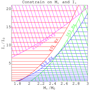
Figure 1: The four constrains Eq. (15)-(18), in the $(M_{*},I_{*})$-plane, labeled with the spin frequency or marked by singularity for Eq. (18). The hashed regions are forbidden. The minimum allowed mass and moment of inertia are around $M\approx 1.93\,M_{\odot}$ and $I_{*}\approx 0.98\,I_{0}$.

All these constrains, Eq. (15)-(18), are summarized and shown in a $(M_{*},I_{*})$-plane depicted in Fig. 1. The hashed regions are forbidden and only a small area in white survives around the first diagonal in the figure. This plot clearly emphasizes the existence of a lower and upper bound for both the mass and moment of inertia. We found the minimum values to be $M_{*\rm min}=1.9\,M_{\odot}$ and $I_{*\rm min}=0.98\,I_{0}$ whereas the maximum ones are $M_{*\rm max}=2.9\,M_{\odot}$ and $I_{*\rm max}=19.1\,I_{0}$. Neutron star structure models predict $I_{*}$ close to or slightly above $I_{0}$ so that we will favor the lower bounds and expect masses in the vicinity of $1.9\,M_{\odot}$.

In a last step, we use the figure-of-merit function $\mathcal{F}$, Eq. (8), to fit the data and also the variation of mass with spin rate according to Eq. (9). We span a vast range in the $(M,I_{*})$-plane to compute the merit function. Note however the subtil change in unknowns compared to the previous analytical study. Now we use a constant mass for the non-rotating limit, $M$, instead of a constant mass for the rotating star, $M_{*}=M+I_{*}\,\Omega_{*}^{2}/2\,c^{2}$. Actually, the discrepancy between both approaches is small and can be neglected at the end of the study.

The results presenting the isocontours of the merit function are summarized in Fig. 2. The resulting region for minimization of $\mathcal{F}$ is marked in red and shapes very similarly to the previous diagram $(M_{*},I_{*})$, Fig. 1. The most probable mass and moment of inertia are $M\approx 2.0-2.2\,M_{\odot}$ and $I_{*}\approx 0.5-1.5\,(10\;\textrm{ km})^{2}\,M_{\odot}$. The best fit according to these values is shown in Fig. 3 where the spin rate is plotted on the x-axis and the twin kHz-QPOs difference normalized to the spin rate is plotted on the y-axis. First, we retrieve the segregation between slow and fast rotators at the correct frequency as expected. Next, for fast spinning stars, the theoretical curve agrees very well with observations. Nevertheless, for slow rotation rates, the spread around unity is significant and cannot be explained in a straightforward way by our predictions. Clearly, some refinement of the model is still needed and under investigations, including other aspects of the plasma flow around an accreting magnetized neutron star.

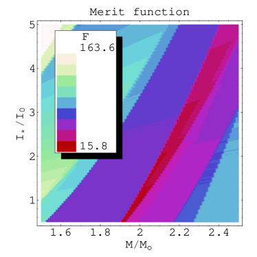
Figure 2: Isocontours of the merit function $\mathcal{F}$ vs the fiducial mass of the non-rotating neutron star $M$, normalized to the solar mass $M_{\odot}$, and vs its moment of inertia $I_{*}$, normalized to $I_{0}=10^{38}\;{\rm kg\,m^{2}}$. The minimum value of $f$ lies around $M\approx 2.0-2.2\,M_{\odot}$ and $I_{*}\approx 1-3\,I_{0}$.

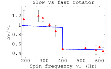
Figure 3: Observations of slow and fast rotators (red triangles) and fit obtained by our model (blue solid line). The best fit parameters are $M\approx 2.0-2.2\,M_{\odot}$ and $I_{*}\approx 1-3\,I_{0}$.

4 Discussion and Conclusion

In this paper, we investigated further the consequences of forced oscillations induced in an accretion disk to explain the twin kHz-QPOs in LMXBs. Our model is able to discriminate between slow and fast rotator as already shown in Pétri (2005a). Moreover, with help on new data from a dozen rotators, we were able to constrain the average mass and moment of inertia of neutron stars. We found for the best fit $M\approx 2.0-2.2\,M_{\odot}$ and $I_{*}\approx 0.5-1.5\,(10\;\textrm{ km})^{2}\,M_{\odot}$. Whereas the moment of inertia gives roughly the same value as those obtained from independent ways by solving the stellar structure with several equations of state (Worley et al., 2008), the neutron star mass appears rather large. This effect could be an artefact of its constancy from one binary system to another. Better fits suggests to look at each system individually and remove the constant mass approximation for the whole set of LMXBs, leading to a spread in the mass distribution function for neutron stars. But this requires a much more detailed separate analysis of each binary with their own specificities (accretion rate, magnetic field strength for instance) and better observations. New time analyzing instruments like the HTRS (High Time Resolution Spectrometer) project on board IXO will give more insights into supra-nuclear matter and strong gravity physics (Barret et al., 2008).

Appendix A Toward a more realistic model

So far our linear parametric resonance model predicts fixed radii where the resonance conditions Eq. (1) are satisfied. Therefore the orbital frequencies remain also constant, leading to fixed kHz-QPOs. This can only be an approximation since oscillations are non-linear and gas or particles drift slowly towards the neutron star due to accretion. In other words, advection increases the orbital and vertical epicyclic frequencies and puts the system (particles) out of resonance. Actually, if non-linear terms are retained, the proper frequency of the vertical excursions depends on the amplitude of these oscillations. Therefore, it is possible that the excitation and proper frequencies adjust themself in such a way to maintain the oscillator in high amplitude motion. We call this a parametric auto-resonance mechanism. Its explanation is given in more details along the following lines.

The idea of non-linear resonance to explain QPO observations has already been discussed by many authors, see for instance Rebusco (2004); Horák (2004, 2005); Abramowicz et al. (2003b). Although they considered a resonance between oscillatory modes different from those relevant to the model presented within this paper, their results show also how non-linear phenomena can drastically improve their models.

Let us see how parametric auto-resonance works. Add a non-linear cubic term in the usual Mathieu equation governing the vertical displacement $z(t)$. Note that, to first order, a quadratic term would not lead to a change in proper frequency with amplitude so a cubic term is more relevant for our discussion. Thus, our non-linear oscillator takes the form below

$$\frac{d^{2}z}{dt^{2}}+\kappa_{\rm z}^{2}(t)\,[1+h\,\cos(m(\Omega(t)-\Omega_{*})\,t)]\,z=\beta\,z^{3}$$ (A1)

$h$ is the strength of the excitation. Now, an important new fact is that the vertical epicyclic $\kappa_{\rm z}(t)$ and orbital $\Omega(t)$ frequencies are time dependent. These variable coefficients mimic the particle radial drift. How does the position of the resonant particles evolve with time due to loss of angular momentum expected from accretion? A simple argument to get the temporal dependence is the following. Assume that the thin accretion disk possesses a power-law axisymmetric surface density $\Sigma(r)$ such that

$$\Sigma(r)=\Sigma_{0}\,\left(\frac{r}{r_{0}}\right)^{\alpha}$$ (A2)

where $\alpha$ is the power law index and $\Sigma_{0}$ the surface density at $r_{0}$. The flow starts to accrete at an initial speed $v_{0}$ (directed radially inwards such that $\vec{v}=-v_{0}\,\vec{e}_{r}$) at radius $r_{0}$. The conservation of mass implies

$$2\,\pi\,r\,\Sigma(r)\,v(r)=2\,\pi\,r_{0}\,\Sigma_{0}\,v_{0}$$ (A3)

Integration with respect to time, using the fact that for a test particle $v(r)=-dr/dt$ (projection along $-\vec{e}_{r}$), we get for $\alpha\neq-2$

$$r(t)=\left[r_{0}^{\alpha+2}-(\alpha+2)\,r_{0}^{\alpha+1}\,v_{0}(t-t_{0})\right]^{\frac{1}{\alpha+2}}$$ (A4)

where $r_{0}=r(t_{0})$ is the initial position of the particle. Specializing to a uniform density disk model, i.e. $\alpha=0$, the particle falls onto the neutron star along the trajectory

$$r(t)=\sqrt{r_{0}^{2}-2\,r_{0}\,v_{0}\,(t-t_{0})}$$ (A5)

For convenience, in the remainder of this paper, we will use this expression for the particle radial path. Furthermore, we make a shift of time by the replacement $(t-t_{0})\to t$. This temporal dependence on radius $r(t)$ governs the time evolution of the orbital $\Omega(t)$ as well as the vertical epicyclic $\kappa_{\rm z}(t)$ frequencies. Parametric auto-resonance will settle in if the excitation is efficient enough to maintain phase locking. In some special cases, we can look for semi-analytical solutions by the method of averaging (Khain & Meerson, 2001). The underlying idea is to smooth the fastest time scale $\Omega(t)$ and to keep track of only the secular amplitude change and phase evolution of the oscillation, compared to an harmonic oscillator.

We apply this technique to our resonance model. First, for small enough times $v_{0}\,t\ll r_{0}$, an expansion of radius and frequencies yields (assuming a non-rotating body, $\tilde{a}=0$)

$$r(t) \approx r_{0}-v_{0}\,t$$ (A6)

$$\Omega(t) \approx \Omega_{0}\,\left(1+\frac{3}{2}\,\frac{v_{0}\,t}{r_{0}}\right)$$ (A7)

$$\Omega_{0} \approx \sqrt{\frac{G\,M}{r_{0}^{3}}}$$ (A8)

$$\kappa_{\rm z}(t) \approx \Omega(t)$$ (A9)

The non-linear parametric resonance model for vertical motion becomes

$$\frac{d^{2}z}{dt^{2}}+\Omega_{0}^{2}\left(1+\frac{3}{2}\frac{v_{0}\,t}{r_{0}}\right)^{2}\left[1+h\cos\left\{m\left(\Omega_{0}\,\left(1+\frac{3}{2}\frac{v_{0}\,t}{r_{0}}\right)-\Omega_{*}\right)t\right\}\right]z=\beta z^{3}$$ (A10)

Next, the method of averaging looks for solutions expanded into $z(t)=A(t)\,\cos\vartheta(t)$, the amplitude being $A(t)$ and the phase being $\vartheta(t)$, $A(t)$ varying on a timescale much longer than the period of oscillations. It is preferable to introduce a new phase defined by

$$\psi=\vartheta-\Omega_{0}\,t$$ (A11)

to get rid of the fastest timescale represented by $\Omega_{0}$. Let us have a look on the behavior of the first resonance. Specializing to this particular case corresponding to $n=1$ and $m=1$, the resonance condition, in the Newtonian limit, is $\Omega_{0}=\Omega_{*}/3$. Inserting into Eq. (A10), the vertical motion satisfies

$$\frac{d^{2}z}{dt^{2}}+\frac{\Omega_{*}^{2}}{9}\,\left(1+\frac{3}{2}\frac{v_{0}\,t}{r_{0}}\right)^{2}\left[1+h\,\cos\left\{\frac{2}{3}\Omega_{*}\,\left(1-\frac{3}{4}\frac{v_{0}\,t}{r_{0}}\right)\,t\right\}\right]z=\beta\,z^{3}$$ (A12)

The straightforward way is to solve numerically this second order differential equation with appropriate initial conditions. We show an example of numerical integration of Eq. (A12) in Fig. 4 when the particle enter in the first resonance, $n=m=1$. The full solution, $z(t)$, is not plotted because of the small timescale, whereas the evolution of the amplitude is shown by a solid blue line, $|z(t)|$. A clear increase of the amplitude with respect to time is demonstrated. This shows that resonance can occur even for variable orbital and excitation frequencies.

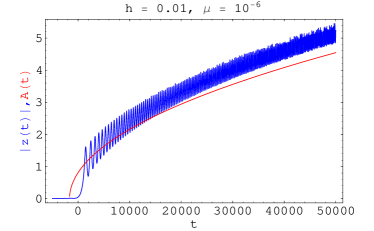
Figure 4: An example of growing oscillation amplitude $|z(t)|$, solid blue line, due to the parametric auto-resonance. The parameters are $h=10^{-2}$, $\beta=10^{-2}$ and $\mu=v_{0}/r_{0}=10^{-6}$. The orbital frequency is normalized to unity $\Omega=1$ or equivalently $\Omega_{*}=3$. The short orbital period of $2\,\pi$ is not plotted. The solid red line shows the quasi-stationary fixed point solution for the amplitude $A(t)$, Eq. (A16), in good agreement with the true solution.

Averaging provides another mean to solve approximately for the amplitude $A$ and the phase $\psi$. For accretion timescales much longer than the orbital motion, which is usually the case, these new unknowns evolve according to

$$\frac{dA}{dt} = \frac{h\,A\,\Omega_{*}\,\sin(2\,\psi)}{12}$$ (A13)

$$\frac{d\psi}{dt} = \frac{h\,\Omega_{*}\,\cos(2\,\psi)}{12}-\frac{9\,\beta\,A^{2}}{8\,\Omega_{*}}+\frac{\Omega_{*}}{2}\,\frac{v_{0}\,t}{r_{0}}$$ (A14)

A stationary solution corresponds mathematically speaking to a fixed point satisfying $\frac{dA}{dt}=\frac{d\psi}{dt}=0$. Inverting this system for the phase and amplitude, we find the real positive amplitude by

$$\sin(2\,\psi) = 0$$ (A15)

$$A(t) = \frac{2}{3}\,\Omega_{*}\,\sqrt{\frac{1}{\beta}\,\left(\frac{v_{0}\,t}{r_{0}}+\frac{h}{6}\right)}$$ (A16)

This analytical solution, solid red line in Fig. 4, agrees very well with the straightforward numerical integration of Eq. (A12). From that, we conclude that oscillations grow slowly as time goes. Simultaneously, the orbital period increases according to Eq. (A7) and consequently so does the kHz-QPO frequency. We recall that this describes the short time evolution of the particle just after entering resonance. In this limit, the fractional increase in the frequency remains small, a few percent. Other resonance, with different $m,n$ will follow the same trend. Accretion and non-linearities allow the QPO peaks to drift towards higher frequencies and release the fixed frequency ratio result.

The analysis of its long term evolution (with the full non-linear time dependence retained) requires more investigation and is left for future work. This discussion aimed at emphasizing that the parametric resonance model extended to more realistic situations met in accretion disks (non linearity and chirped frequency) can explain an increase in the observed kHz-QPO frequencies by parametric auto-resonance.

To conclude, representative references about the real behaviour of the QPO amplitudes and coherence times can be found in Barret et al. (2005a, b); Méndez (2006). Finally, we refer to Török (2009) and Horák et al. (2009) for a discussion on the relation between the strength of the twin QPOs and its possible explanation within the framework of a non-linear resonance theory.

The study done in this appendix is very preliminary and will be included in an extended model of our parametric resonance.

References

- Abramowicz et al. (2007) Abramowicz, M., Kluzniak, W., Bursa, M., et al. 2007, in Revista Mexicana de Astronomia y Astrofisica Conference Series, Vol. 27, Revista Mexicana de Astronomia y Astrofisica Conference Series, 8–17
- Abramowicz et al. (2005a) Abramowicz, M. A., Barret, D., Bursa, M., et al. 2005a, in RAGtime 6/7: Workshops on black holes and neutron stars, ed. S. Hledík & Z. Stuchlík, 1–9
- Abramowicz et al. (2005b) Abramowicz, M. A., Barret, D., Bursa, M., et al. 2005b, Astronomische Nachrichten, 326, 864
- Abramowicz et al. (2003a) Abramowicz, M. A., Bulik, T., Bursa, M., & Kluźniak, W. 2003a, A&A, 404, L21
- Abramowicz et al. (2003b) Abramowicz, M. A., Karas, V., Kluzniak, W., Lee, W. H., & Rebusco, P. 2003b, PASJ, 55, 467
- Aliev & Galtsov (1981) Aliev, A. N. & Galtsov, D. V. 1981, General Relativity and Gravitation, 13, 899
- Barret et al. (2008) Barret, D., Belloni, T., Bhattacharyya, S., et al. 2008, in Society of Photo-Optical Instrumentation Engineers (SPIE) Conference Series, Vol. 7011, Society of Photo-Optical Instrumentation Engineers (SPIE) Conference Series
- Barret & Boutelier (2008) Barret, D. & Boutelier, M. 2008, New Astronomy Review, 51, 835
- Barret et al. (2005a) Barret, D., Olive, J., & Miller, M. C. 2005a, MNRAS, 361, 855
- Barret et al. (2005b) Barret, D., Olive, J., & Miller, M. C. 2005b, Astronomische Nachrichten, 326, 808
- Belloni et al. (2005) Belloni, T., Méndez, M., & Homan, J. 2005, A&A, 437, 209
- Belloni et al. (2007) Belloni, T., Méndez, M., & Homan, J. 2007, MNRAS, 101
- Bhattacharyya (2010) Bhattacharyya, S. 2010, ArXiv e-prints
- Boutelier et al. (2010) Boutelier, M., Barret, D., Lin, Y., & Török, G. 2010, MNRAS, 401, 1290
- Camenzind (2007) Camenzind, M. 2007, Compact objects in astrophysics : white dwarfs, neutron stars, and black holes, ed. M. Camenzind
- Casares et al. (2006) Casares, J., Cornelisse, R., Steeghs, D., et al. 2006, MNRAS, 373, 1235
- Deloye et al. (2008) Deloye, C. J., Heinke, C. O., Taam, R. E., & Jonker, P. G. 2008, MNRAS, 391, 1619
- Ghosh (2007) Ghosh, P. 2007, Rotation and Accretion Powered Pulsars, ed. Ghosh, P. (World Scientific Publishing Co)
- Haensel et al. (2007) Haensel, P., Potekhin, A. Y., & Yakovlev, D. G., eds. 2007, Astrophysics and Space Science Library, Vol. 326, Neutron Stars 1 : Equation of State and Structure
- Hartle & Thorne (1968) Hartle, J. B. & Thorne, K. S. 1968, ApJ, 153, 807
- Horák (2004) Horák, J. 2004, in RAGtime 4/5: Workshops on black holes and neutron stars, ed. S. Hledík & Z. Stuchlík, 91–110
- Horák (2005) Horák, J. 2005, Astronomische Nachrichten, 326, 824
- Horák et al. (2009) Horák, J., Abramowicz, M. A., Kluźniak, W., Rebusco, P., & Török, G. 2009, A&A, 499, 535
- Kato et al. (1998) Kato, S., Fukue, J., & Mineshige, S., eds. 1998, Black-hole accretion disks
- Khain & Meerson (2001) Khain, E. & Meerson, B. 2001, Phys. Rev. E, 64, 036619
- Kluzniak et al. (2007) Kluzniak, W., Abramowicz, M. A., Bursa, M., & Török, G. 2007, in Revista Mexicana de Astronomia y Astrofisica, vol. 27, Vol. 27, Revista Mexicana de Astronomia y Astrofisica, vol. 27, 18–25
- Kluzniak et al. (1990) Kluzniak, W., Michelson, P., & Wagoner, R. V. 1990, ApJ, 358, 538
- Kluzniak & Wagoner (1985) Kluzniak, W. & Wagoner, R. V. 1985, ApJ, 297, 548
- Lattimer (2007) Lattimer, J. M. 2007, Ap&SS, 308, 371
- Lattimer & Prakash (2007) Lattimer, J. M. & Prakash, M. 2007, Phys. Rep., 442, 109
- Lyford et al. (2003) Lyford, N. D., Baumgarte, T. W., & Shapiro, S. L. 2003, ApJ, 583, 410
- Méndez (2006) Méndez, M. 2006, MNRAS, 371, 1925
- Méndez & Belloni (2007) Méndez, M. & Belloni, T. 2007, MNRAS, 381, 790
- Miller et al. (1998) Miller, M. C., Lamb, F. K., & Psaltis, D. 1998, ApJ, 508, 791
- Nice (2006) Nice, D. J. 2006, Advances in Space Research, 38, 2721
- Ozel et al. (2010) Ozel, F., Baym, G., & Guver, T. 2010, ArXiv e-prints
- Page & Reddy (2006) Page, D. & Reddy, S. 2006, Annual Review of Nuclear and Particle Science, 56, 327
- Pétri (2005a) Pétri, J. 2005a, A&A, 439, L27
- Pétri (2005b) Pétri, J. 2005b, A&A, 443, 777
- Rebusco (2004) Rebusco, P. 2004, PASJ, 56, 553
- Rezania & Samson (2005) Rezania, V. & Samson, J. C. 2005, A&A, 436, 999
- Shapiro & Teukolsky (1983) Shapiro, S. L. & Teukolsky, S. A. 1983, Black holes, white dwarfs, and neutron stars: The physics of compact objects (Research supported by the National Science Foundation. New York, Wiley-Interscience, 1983, 663 p.)
- Stella & Vietri (1999) Stella, L. & Vietri, M. 1999, Physical Review Letters, 82, 17
- Thorsett & Chakrabarty (1999) Thorsett, S. E. & Chakrabarty, D. 1999, ApJ, 512, 288
- Török (2009) Török, G. 2009, A&A, 497, 661
- Török et al. (2008a) Török, G., Abramowicz, M. A., Bakala, P., et al. 2008a, Acta Astronomica, 58, 15
- Török et al. (2008b) Török, G., Abramowicz, M. A., Bakala, P., et al. 2008b, Acta Astronomica, 58, 113
- Török et al. (2010) Török, G., Bakala, P., Šrámková, E., Stuchlík, Z., & Urbanec, M. 2010, ApJ, 714, 748
- Török & Stuchlík (2005) Török, G. & Stuchlík, Z. 2005, A&A, 437, 775
- van der Klis (2006a) van der Klis, M. 2006a, Advances in Space Research, 38, 2675
- van der Klis (2006b) van der Klis, M. 2006b, Rapid X-ray Variability, ed. Lewin, W. H. G. & van der Klis, M., 39–112
- van der Klis (2008) van der Klis, M. 2008, in American Institute of Physics Conference Series, Vol. 1068, American Institute of Physics Conference Series, ed. R. Wijnands, D. Altamirano, P. Soleri, N. Degenaar, N. Rea, P. Casella, A. Patruno, & M. Linares, 163–173
- Worley et al. (2008) Worley, A., Krastev, P. G., & Li, B. 2008, ApJ, 685, 390
- Yin et al. (2007) Yin, H. X., Zhang, C. M., Zhao, Y. H., et al. 2007, A&A, 471, 381
- Zhang (2004) Zhang, C. 2004, A&A, 423, 401
- Zhang (2009) Zhang, C. M. 2009, Astronomische Nachrichten, 330, 398
- Zhang et al. (2007) Zhang, C. M., Yin, H. X., Kojima, Y., et al. 2007, MNRAS, 374, 232
- Zhang et al. (2006) Zhang, C. M., Yin, H. X., Zhao, Y. H., Zhang, F., & Song, L. M. 2006, MNRAS, 366, 1373