Theory of Fiber Optic Raman Polarizers

Abstract

The theoretical description of a Raman amplifier based on the vector model of randomly birefringent fibers is proposed and applied to the characterization of Raman polarizers. The Raman polarizer is a special type of Raman amplifier with the property of producing a highly repolarized beam when fed by relatively weak and unpolarized light.

¹Department of Information Engineering, Università di Brescia, Via Branze 38, 25123 Brescia, Italy
²Department of Physics, St.-Petersburg State University, Petrodvoretz, St.-Petersburg, 198504, Russia
³Instituto de Optica, Consejo Superior de Investigaciones Cientificas (CSIC), 28006 Madrid, Spain

victor.kozlov@email.com

230.5440; 060.4370; 230.1150; 230.4320

Polarization-dependent gain (PDG), an intrinsic characteristic of optical fiber-based Raman amplifiers, is generally considered an unwanted feature for telecom-related applications. Very recently such opinion about the role of PDG was reversed, as the quest for higher transmission capacities brings to the forefront the need for polarization multiplexing protocols and polarization-controlling devices. Indeed, Martinelli et. al. demonstrated in Ref. [1] such a device, called Raman polarizer, which selectively amplifies only one polarization mode of the input beam, and thereby yields only this mode at the output, independently of the input state of polarization (SOP) of the signal beam. The development of a simple, yet rigorous as well as computer-friendly theory of Raman polarizers along with the scheme for their characterization is thus the purpose of this Letter.

Telecom fibers are randomly birefringent fibers. Representative examples of vector theories of Raman amplifiers developed for telecom fibers can be found in Refs. [2, 3]. The analytic theory of Ref. [2] is limited by the condition that the beat length $L_{B}$ is smaller than the birefringence correlation length $L_{c}$, and therefore their validity is questionable when applied to Raman polarizers, which as we shall see require the opposite inequality $L_{B}\gg L_{c}$. The full-scale numerical approach in Ref. [3] accurately models a randomly birefringent fiber as consisting of fiber spans with randomly distributed values and orientations of the birefringence. Typically, thousands of such realizations are required for getting an accurate statistics. Hence the required computer time is three to four orders of magnitude longer than for the numerical modeling involved in the theory presented below. In addition to the much faster performance, our theory is formulated in terms of a set of deterministic differential equations, and as such allows for a simple physical interpretation.

Starting with the equations of motion formulated by Lin and Agrawal in Ref. [2] we extend the one-beam model of the stochastic fiber proposed by Wai and Menyuk in Ref. [4] to two beams interacting not only via Kerr, but also via Raman effect. Detailed derivations can be found in Ref. [5], while here we only provide the final equation formulated for the Stokes vector $S^{(s)}=(S_{1}^{(s)},\,S_{2}^{(s)},\,S_{3}^{(s)})$ of the signal beam:

$$\left(\partial_{z}+\beta^{\prime}(\omega_{s})\partial_{t}\right)S^{(s)}=-\alpha_{s}S^{(s)}+$$

$$\gamma(\omega_{s})\left(S^{(s)}\times\boldsymbol{J}_{S}^{(s)}(z)S^{(s)}+S^{(s)}\times\boldsymbol{J}_{X}(z)S^{(p)}\right)$$

$$+\epsilon_{s}g_{0}\left(S_{0}^{(p)}J_{R0}S^{(s)}+S_{0}^{(s)}\boldsymbol{J}_{R}(z)S^{(p)}\right)\,.$$ (1)

The components of the Stokes vector are written in terms of the two polarization components $V_{s1}$ and $V_{s2}$ of the slowly varying signal field in the appropriate reference frame, as $S_{1}^{s}=V_{s1}V_{s2}^{*}+V_{s1}^{*}V_{s2}$, $S_{2}^{s}=i(V_{s1}^{*}V_{s2}-V_{s1}V_{s2}^{*})$, $S_{3}^{s}=|V_{s1}|^{2}-|V_{s2}|^{2}$. Similar equations and definitions (with labels $p$ and $s$ interchanged) hold for the pump beam. $\gamma(\omega_{s})$ is the Kerr coefficient of the fiber at frequency $\omega_{s}$ of the signal beam; $g_{0}$ is the Raman gain coefficient; $\beta^{\prime}(\omega_{s})$ is the inverse group velocity of the signal beam; $\alpha_{s}$ is the attenuation coefficient; $\epsilon_{s}=1$; $\epsilon_{p}=-\omega_{p}/\omega_{s}$. Matrices in the Eq. (1) are all diagonal with elements $\boldsymbol{J}_{R}=\hbox{diag}(J_{R1},\,J_{R2},\,J_{R3})$, $\boldsymbol{J}_{X}=\hbox{diag}(J_{X1},\,J_{X2},\,J_{X3})$, $\boldsymbol{J}_{S}=\hbox{diag}(J_{S1},\,J_{S2},\,J_{S3})$. Here $J_{R1}=\langle\hbox{Re}(u_{14}^{2}-u_{10}^{2})\rangle$, $J_{R2}=-\langle\hbox{Re}(u_{14}^{2}+u_{10}^{2})\rangle$, $J_{R3}=-\langle|u_{14}|^{2}-|u_{10}|^{2}\rangle$, $J_{X1}=\frac{2}{3}\langle\hbox{Re}(u_{10}^{2}+u_{13}^{2}-u_{9}^{2}-u_{14}^{2})\rangle$, $J_{X2}=\frac{2}{3}\langle\hbox{Re}(u_{10}^{2}+u_{14}^{2}-u_{9}^{2}-u_{13}^{2})\rangle$, $J_{X3}=\frac{2}{3}\langle|u_{9}|^{2}+|u_{14}|^{2}-|u_{13}|^{2}-|u_{10}|^{2}\rangle$, $J_{S1}=\frac{1}{3}\langle\hbox{Re}(u_{6}^{2})\rangle$, $J_{S2}=-\frac{1}{3}\langle\hbox{Re}(u_{6}^{2})\rangle$, $J_{S3}=\frac{1}{3}\left[3\langle u_{3}^{2}\rangle-1\right]$, and also $J_{R0}=\langle|u_{10}|^{2}+|u_{14}|^{2}\rangle$. The three groups of coefficients $\{\langle u_{1}^{2}\rangle,\,\langle u_{2}^{2}\rangle,\,\langle u_{3}^{2}\rangle\}$, $\{\langle\hbox{Re}^{2}(u_{4})\rangle,\,\langle\hbox{Re}^{2}(u_{5})\rangle,\,\langle\hbox{Re}^{2}(u_{6})\rangle\}$, and $\{\langle\hbox{Im}^{2}(u_{4})\rangle,\,\langle\hbox{Im}^{2}(u_{5})\rangle,\,\langle\hbox{Im}^{2}(u_{6})\rangle\}$ obey equations

$$\partial_{z}G_{1}=-2L_{c}^{-1}(G_{1}-G_{2})\,,$$

$$\partial_{z}G_{2}=2L_{c}^{-1}(G_{1}-G_{2})-4\Delta\beta(\omega_{s})G_{4}\,,$$

$$\partial_{z}G_{3}=4\Delta\beta(\omega_{s})G_{4}\,,$$

$$\partial_{z}G_{4}=-L_{c}^{-1}G_{4}+2\Delta\beta(\omega_{s})(G_{2}-G_{3})\,,$$

when we associate them with $\{G_{1},\,G_{2},\,G_{3}\}$ respectively. Initial conditions are respectively $(1,\,0,\,0)$, $(0,\,1,\,0)$, and $(0,\,0,\,1)$. In turn, the rest four groups of coefficients $\{\langle\hbox{Re}^{2}(u_{7})\rangle,\,\langle\hbox{Re}^{2}(u_{8})\rangle,\,\langle\hbox{Re}^{2}(u_{9}),\,\langle\hbox{Re}^{2}(u_{10})\rangle\}$, $\{\langle\hbox{Im}^{2}(u_{7})\rangle,\,\langle\hbox{Im}^{2}(u_{8})\rangle,\,\langle\hbox{Im}^{2}(u_{9}),\,\langle\hbox{Im}^{2}(u_{10})\rangle\}$, $\{\langle\hbox{Re}^{2}(u_{11})\rangle,\,\langle\hbox{Re}^{2}(u_{12})\rangle,\,\langle\hbox{Re}^{2}(u_{13}),\,\langle\hbox{Re}^{2}(u_{14})\rangle\}$, and $\{\langle\hbox{Im}^{2}(u_{11})\rangle,\,\langle\hbox{Im}^{2}(u_{12})\rangle,\,\langle\hbox{Im}^{2}(u_{13}),\,\langle\hbox{Im}^{2}(u_{14})\rangle\}$, can be found from equations

$$\partial_{z}G_{1}=-2L_{c}^{-1}(G_{1}-G_{2})+2\Delta_{-}G_{5}\,,$$

$$\partial_{z}G_{2}=2L_{c}^{-1}(G_{1}-G_{2})-2\Delta_{+}G_{6}\,,$$

$$\partial_{z}G_{3}=2\Delta_{+}G_{6}\,,$$

$$\partial_{z}G_{4}=-2\Delta_{-}G_{5}\,,$$

$$\partial_{z}G_{5}=\Delta_{-}(G_{4}-G_{1})-L_{c}^{-1}G_{5}\,,$$

$$\partial_{z}G_{6}=\Delta_{+}(G_{2}-G_{3})-L_{c}^{-1}G_{6}\,,$$

when we associate them with $\{G_{1},\,G_{2},\,G_{3},\,G_{4}\}$, with initial conditions as $(1,\,0,\,0,\,0)$, $(0,\,0,\,0,\,1)$, $(0,\,1,\,0,\,0)$, and $(0,\,0,\,1,\,0)$, respectively. Here, $\Delta_{\pm}\equiv\Delta\beta(\omega_{p})\pm\Delta\beta(\omega_{s})$, where $\Delta\beta(\omega_{s})$ [$\Delta\beta(\omega_{p})$] is the magnitude of the birefringence at frequency $\omega_{s}$ ($\omega_{p}$). The power of the signal beam defined as $S_{0}^{(s)}=\left({S_{1}^{(s)}}^{2}+{S_{2}^{(s)}}^{2}+{S_{3}^{(s)}}^{2}\right)^{1/2}$ obeys the equation

$$\left(\partial_{z}+\beta^{\prime}(\omega_{s})\partial_{t}\right)S_{0}^{(s)}=-\alpha_{s}S_{0}^{(s)}+g_{0}\Big{(}J_{R0}S_{0}^{(s)}S_{0}^{(p)}$$

$$+J_{R1}S_{1}^{(s)}S_{1}^{(p)}+J_{R2}S_{2}^{(s)}S_{2}^{(p)}+J_{R3}S_{3}^{(s)}S_{3}^{(p)}\Big{)}\,.$$ (2)

Eqs. (1) and (2) for the signal (and pump) fields are the key finding of our study. These equations are valid for a wide range of parameters and regimes, for undepleted as well as with a depleted pump. The only limitation is that the total length of the fiber $L$ and/or the nonlinear length $L_{NL}=[\gamma(\omega_{s})S_{0}^{(p)}]^{-1}$ be longer than the correlation length $L_{c}$. Eqs. (1) and (2) can be easily solved numerically, in particular in the co-propagating configuration and undepleted pump regime, which is of interest to us here. In this case the $z$-dependent elements on the diagonals of the SPM, XPM and Raman matrices, $\boldsymbol{J}_{S}$, $\boldsymbol{J}_{X}$, and $\boldsymbol{J}_{R}$, are obtained as previously discussed.

When doing this, we found that both SPM and XPM effects have virtually no impact on the performance of Raman polarizers operating in the undepleted pump regime. In contrast, the form of the Raman matrix is of paramount importance. The larger the coefficients on the diagonal, the stronger the PDG. For moderate values of the polarization mode dispersion (PMD) coefficient, Raman diagonal terms only take appreciable values near the fiber input, as illustrated in Fig. 1. Therefore, the power of the pump beam is to be high, in order to provide significant amplification over the first few hundreds meters of the fiber.

For analyzing the performance of Raman polarizers we identify three characteristic quantities: the degree of polarization (DOP) of the outcoming signal beam, its SOP, and the overall signal gain. The DOP and SOP characteristics are illustrated in Fig. 2. Since the signal SOP depends on the pump SOP, it is reasonable to define a quantity that measures the relative difference between these two SOPs. As usual, such quantity is the alignment parameter

$$A_{\uparrow\uparrow}\equiv\frac{\left\langle S_{1}^{(s)}S_{1}^{(p)}+S_{2}^{(s)}S_{2}^{(p)}+S_{3}^{(s)}S_{3}^{(p)}\right\rangle}{S_{0}^{(s)}S_{0}^{(p)}}\,,$$ (3)

which is the cosine of the angle between the pump and the signal Stokes vectors, averaged over the ensemble of beams with random SOPs which models the unpolarized signal beam. The hypothesis that the signal SOP is attracted to the pump SOP is rooted in the model of isotropic fibers, in which $J_{R1}=J_{R2}=J_{R2}=1$. In randomly birefringent fibers, the equality and even positivity of the three elements is not always the case, as exemplified in the plot of Fig. 1. In these cases, it is remarkable that the signal SOP is attracted to an SOP which is different from that of the pump. In spite of this observation, we found that for ideal Raman polarizers (those with DOP$>0.9$), and in the range of lengths $0.001<L_{B}<0.05$ and $0.0001<L_{c}<0.05$, given here in km, the signal SOP on average is attracted to the pump SOP, see Fig. 2. This is not the case in the counter-propagating configuration, for which the appropriate alignment parameter $A_{\uparrow\downarrow}$ is different from that given in Eq. (3), see [5]. Moreover, the performance of Raman polarizers (namely, DOP) sensitively depends on the pump SOP, as demonstrated in Fig. 3.

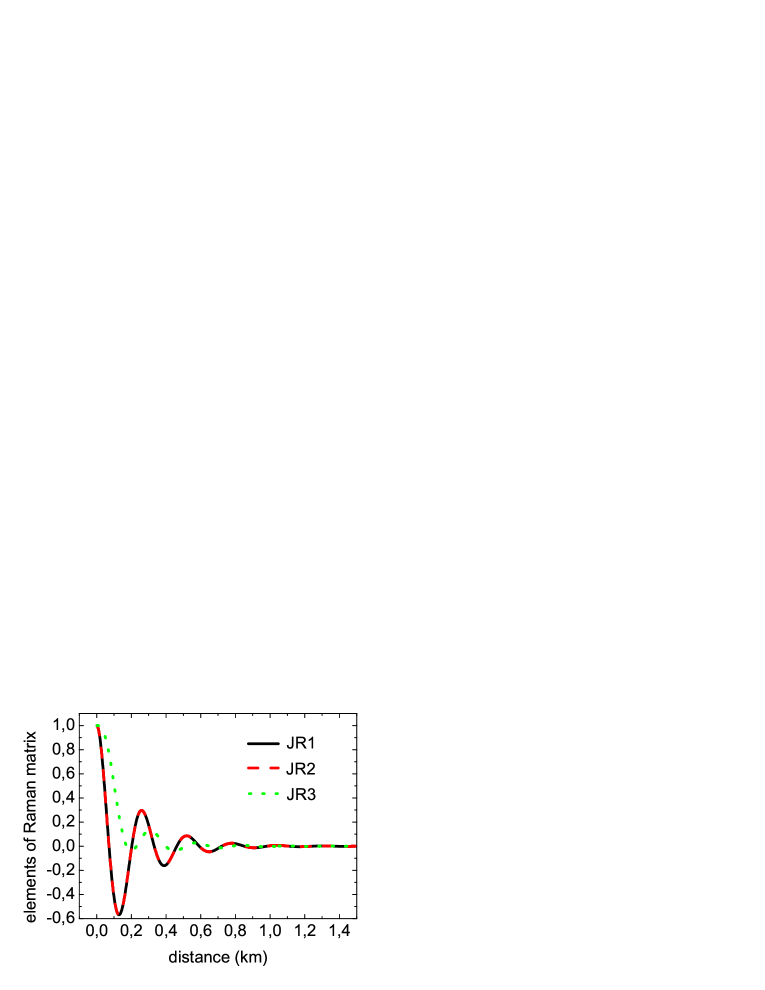
Figure 1: Elements of the Raman matrix ($J_{R1}$ – black solid, $J_{R2}$ – red dashed, and $J_{R3}$ – green dotted) as function of distance in the fiber for $L_{B}(\omega_{p})=0.016$ km and $L_{c}=0.05$ km. (note that the black solid and red dashed curves coincide, i.e. $J_{R1}=J_{R2}$.)

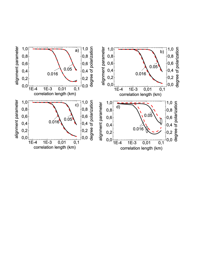
Figure 2: DOP of the signal beam (black, solid) and alignment parameter $A_{\uparrow\uparrow}$ (red, dashed) as function of correlation length $L_{c}$ for the four SOPs of the pump beam: a) $(1/\sqrt{3})(1,\,1,\,1)$; b) $(1,\,0,\,0)$; c) $(0,\,1,\,0)$; d) $(0,\,0,\,1)$. Here and in Figs. 3 and 4, the value of the beat length $L_{B}(\omega_{p})$ is indicated on the plots in km. The two ellipses on plot d) indicate one (of infinitely many) pair of points with equal PMD coefficients. Other parameters are (also used in Figs. 3, 4): input signal power $1$ $\mu$m; input pump power $8$ W; $g_{0}=0.6$ (W$\cdot$km)^-1; $\gamma=1$ (W$\cdot$km)^-1; $\alpha=0.2$ dB/km; $L=1.5$ km.

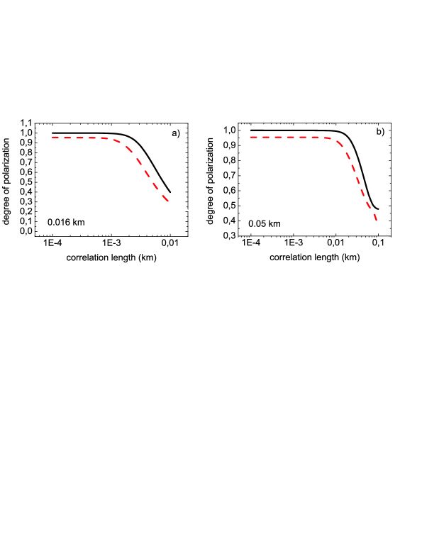
Figure 3: DOP of the signal beam for two SOPs of the pump beam which either maximize (black, solid) or minimize (red, dashed) the signal DOP. For each value of $L_{c}$ we perform a separate search for these two SOPs.

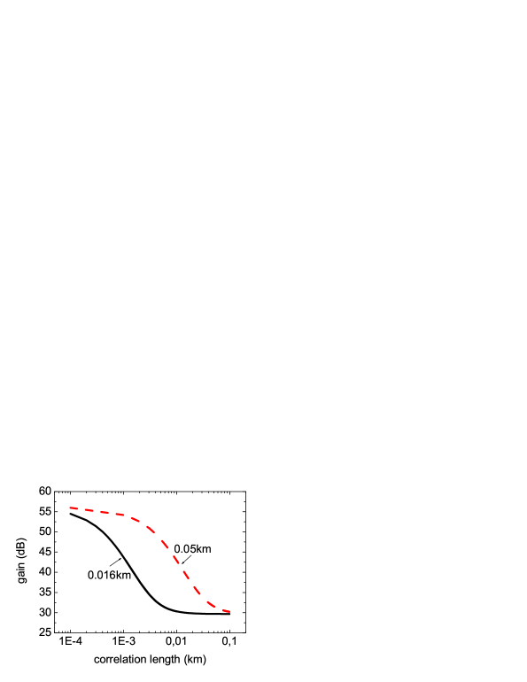
Figure 4: Average Raman polarizer gain as a function of the correlation length. The pump SOP is $(1,\,0,\,0)$ and the signal beam is initially unpolarized.

Another important practical issue is the selection of fibers for Raman polarizers. The main parameter in this selection is the value of the PMD coefficient. In this respect we found that for obtaining a signal DOP close to unity (i.e., $>0.99$) the PMD coefficient should be less than $0.0145$ ps$/\sqrt{\hbox{km}}$ for, say, $8$ W of pump power (as in Ref. [1]). Nevertheless we found that the PMD coefficient does not always provide full information about the fiber. For example in Fig. 2(d) we can see that two fibers with equal PMD coefficients exhibit a different performance as Raman polarizers. In one case, the DOP is $0.25$, in the other – $0.45$. For this reason, it is preferable to consider the beat and correlation lengths separately, rather than combining them into the single PMD coefficient, which for our model is expressed as [4]: $D_{p}=2\sqrt{2}\pi\sqrt{L_{c}}/(L_{B}\omega_{s})$.

The third characteristic of Raman polarizers is Raman gain, see Fig. 4. Even for a $1.5$ km long fiber with $8$ W of pump power we may have an enormous $55$ dB gain that is almost twice the gain of the same Raman amplifier, but with a high value of the PMD coefficient. This means that Raman polarizers are simultaneously very efficient Raman amplifiers. Such values of gain are obtained in the undepleted regime, i.e. for input signal powers in the $\mu$W range. For the mW range which is typical of telecom applications the analysis necessarily enters the depleted pump regime, to which our theory can also be readily applied.

In conclusion, we presented a theory for describing the interaction of two optical beams in randomly birefringent fibers via Kerr and Raman effects, and applied it to the quantification of the performance of Raman polarizers.

We thank L. Palmieri for valuable comments. This work was carried out in the framework of the ”Scientific Research Project of Relevant National Interest” (PRIN 2008) entitled ”Nonlinear cross-polarization interactions in photonic devices and systems” (POLARIZON), and in the framework of the 2009 Italy-Spain integrated action ”Nonlinear Optical Systems and Devices” (HI2008-0075).

References

• [1] M. Martinelli, M. Cirigliano, M. Ferrario, L. Marazzi, and P. Martelli, Evidence of Raman-induced polarization pulling, Opt. Express, 17, 947-955, 2009.
• [2] Q. Lin and G. P. Agrawal, Vector theory of stimulated Raman scattering and its applications to fiber-based Raman amplifiers, J. Opt. Soc. Amer., B 20, 1616-1631, 2003.
• [3] A. Galtarossa, L. Palmieri, M. Santagiustina, and L. Ursini, Polarized backward Raman amplification in randomly birefringent fibers, J. Lightw. Techn., 24, no. 11, 4055-4063, 2006.
• [4] P. K. A.Wai and C. R. Menyuk, Polarization mode dispersion, decorrelation and diffusion in optical fibers with randomly varying birefringence, J. Lightw. Technol., 14, no. 2, 148 157, 1996.
• [5] V. V. Kozlov, J. Nu$\bar{\hbox{n}}$o, J. D. Ania-Casta$\tilde{\hbox{n}}$ón, and S. Wabnitz, Theoretical study of fiber-based Raman polarizers with counterpropagating beams, http://arxiv.org/abs/1009.0446.