Information geometry of density matrices and state estimation

Abstract

Given a pure state vector $|x\rangle$ and a density matrix ${\hat{\rho}}$, the function $p(x|{\hat{\rho}})=\langle x|{\hat{\rho}}|x\rangle$ defines a probability density on the space of pure states parameterised by density matrices. The associated Fisher-Rao information measure is used to define a unitary invariant Riemannian metric on the space of density matrices. An alternative derivation of the metric, based on square-root density matrices and trace norms, is provided. This is applied to the problem of quantum-state estimation. In the simplest case of unitary parameter estimation, new higher-order corrections to the uncertainty relations, applicable to general mixed states, are derived.

The structure of the space ${\mathcal{D}}$ of density matrices is of considerable interest in quantum information theory and related disciplines such as quantum tomography and quantum statistical inference. While substantial progress has been made in unravelling the structure of ${\mathcal{D}}$ Hubner ; BZ ; Petz ; Uhlmann ; Hansen , the subject remains difficult, partly because of the complicated structure of ${\mathcal{D}}$, which is a manifold with a boundary given by degenerate density matrices. The purpose of the present paper is to reveal the existence of a remarkably simple dual metric structure over the space of pure and mixed states, and to apply this to obtain new higher-order corrections to Heisenberg uncertainty relations for general mixed states.

The idea of the dual metric structure can be sketched as follows. If $|x\rangle$ denotes a normalised pure state vector and ${\hat{\rho}}$ a generic density matrix, then the expectation $\langle x|{\hat{\rho}}|x\rangle$ defines a probability density function either on the space of pure states parameterised by density matrices, or on the space of density matrices parameterised by pure states. Hence, methods of information geometry Rao ; Amari ; Brody0 can be employed to define a pair of Riemannian metrics, one for the pure state space and one for the space of density matrices.

An alternative formulation is to use the trace norm and matrix algebra associated with the Hermitian square-root map ${\hat{\rho}}\to{\hat{\xi}}=\surd{\hat{\rho}}$. It is shown that if ${\hat{\xi}}$ is parameterised by a pure state so that ${\hat{\xi}}={\hat{\rho}}$, then the associated information metric is the Fubini-Study metric; whereas if ${\hat{\xi}}$ is parameterised by a generic density matrix, then we recover the information metric on ${\mathcal{D}}$. Apart from these two extremes, however, there are many other cases of considerable interest. Typically, in a problem of quantum state estimation, the density matrix ${\hat{\rho}}(\theta)$ depends on one or several unknown parameters $\{\theta^{i}\}$ that are to be estimated. The Fisher-Rao information metric $4\,{\rm tr}[\partial_{i}{\hat{\xi}}(\theta)\partial_{j}{\hat{\xi}}(\theta)]$, where $\partial_{i}=\partial/\partial\theta^{i}$, then determines the covariance lower bound of the parameter estimates. In the simplest case in which ${\hat{\rho}}(\theta)$ represents a one-parameter unitary curve in the space of density matrices (e.g., $\theta$ represents time), the quantum Fisher-Rao metric coincides with the “skew information” defined by Wigner and Yanase WY . By this device we are able to extend the results of BC ; FN ; caianiello ; Brody1 ; Luo ; Luo3 on quantum statistical inference. In particular, we derive: (a) a variance lower bound for general mixed states, which is sharper than the previously known ones that are expressed in terms of the skew information; (b) the quantum-mechanical analogue of the conditional variance representation in terms of the skew information measures; and (c) higher-order corrections to the uncertainty lower bound for mixed states, whereby the concept of higher-order skew information measures are introduced.

Consider a finite, $n$-dimensional quantum system. The space of pure states ${\mathit{\Gamma}}$ is the space of rays through the origin of ${\mathds{C}}(n)$, which is just the complex projective space equipped with the unitary invariant Fubini-Study metric. We let ${\mathcal{D}}$ denote the space of density matrices on ${\mathds{C}}(n)$. Every density matrix defines a positive scalar function $\langle x|{\hat{\rho}}|x\rangle$ on ${\mathit{\Gamma}}$, and this, properly normalised with respect to the Fubini-Study volume element, yields a probability density on ${\mathit{\Gamma}}$. Since, by the real polarisation identity, a density matrix is uniquely determined by the totality of its expectation values, these probability distributions are parameterised by ${\mathcal{D}}$ in a one-to-one fashion. Hence we can use the Hellinger distances between these distributions and obtain an information metric on ${\mathcal{D}}$ to investigate properties of ${\mathcal{D}}$, which are directly related with the physical significance of density matrices. The dual picture emerges from the converse construction: Given any $|x\rangle\in{\mathit{\Gamma}}$, one obtains a nonzero nonnegative function $\langle x|{\hat{\rho}}|x\rangle$ on ${\mathcal{D}}$, which defines, when properly normalised, a set of probability distributions on ${\mathcal{D}}$. This likewise yields an information metric on ${\mathit{\Gamma}}$. By considerations of symmetry and invariance, using the unitary structure of ${\mathds{C}}^{n}$, one can perceive that this a priori new metric on ${\mathit{\Gamma}}$ can only be the Fubini-Study metric.

If one assumes the Schrödinger equations of motion $|x(t)\rangle=\exp(-\mbox{$\rm i$}{\hat{H}}t)|x(0)\rangle$ on ${\mathit{\Gamma}}$ and the Heisenberg equations of motion ${\hat{\rho}}(t)=\exp(-\mbox{$\rm i$}{\hat{H}}t){\hat{\rho}}(0)\exp(\mbox{$\rm i$}{\hat{H}}t)$ on ${\mathcal{D}}$, then the following conclusions can be drawn. The evolution on ${\mathit{\Gamma}}$ is isometric with respect to the Fubini-Study metric (known as Wigner’s theorem), and, moreover, the evolution on ${\mathcal{D}}$ is isometric with respect to the information metric. Thus, we have a complete reciprocity between the Schrödinger dynamics on ${\mathit{\Gamma}}$, equipped with the Fubini-Study metric, and the Heisenberg dynamics on ${\mathcal{D}}$, endowed with the information metric.

The components of these information metrics, with respect to a given choice of coordinate system, can be calculated by use of the standard expression for the Fisher-Rao metric. Let us write $\{x^{\mu}\}_{\mu=1,\ldots,2n-2}$ for the coordinates on ${\mathit{\Gamma}}$ with volume element $\mbox{$\rm d$}v_{x}$, and $\{\rho^{a}\}_{a=1,\ldots,n^{2}-1}$ for the coordinates on ${\mathcal{D}}$ with volume element $\mbox{$\rm d$}V_{\rho}$. Likewise, we write $p(x|{\hat{\rho}})\propto\langle x|{\hat{\rho}}|x\rangle$ for the normalised density on ${\mathit{\Gamma}}$ and $P({\hat{\rho}}|x)\propto\langle x|{\hat{\rho}}|x\rangle$ for the normalised density on ${\mathcal{D}}$. Then the information metric $G_{ab}$ on ${\mathcal{D}}$ is given by

$$G_{ab}({\hat{\rho}})=\int_{\mathit{\Gamma}}\frac{1}{p(x|{\hat{\rho}})}\frac{\partial p(x|{\hat{\rho}})}{\partial\rho^{a}}\frac{\partial p(x|{\hat{\rho}})}{\partial\rho^{b}}\,\mbox{$\rm d$}v_{x}.$$ (1)

Similarly, the information (Fubini-Study) metric $g_{\mu\nu}$ on ${\mathit{\Gamma}}$ is given by

$$g_{\mu\nu}(x)=\int_{\mathcal{D}}\frac{1}{P({\hat{\rho}}|x)}\frac{\partial P({\hat{\rho}}|x)}{\partial x^{\mu}}\frac{\partial P({\hat{\rho}}|x)}{\partial x^{\nu}}\,\mbox{$\rm d$}V_{\rho}.$$ (2)

We therefore have two statistical manifolds, ${\mathit{\Gamma}}$ with the metric $g_{\mu\nu}$, and ${\mathcal{D}}$ with the metric $G_{ab}$; each of these is represented by probability distributions on the other.

The duality of information metrics leads to integral representations for observable expectations. Let us consider trace-free observables ${\hat{A}}$. Defining $A(x)=\langle x|{\hat{A}}|x\rangle$ and $A({\hat{\rho}})={\rm tr}({\hat{\rho}}{\hat{A}})$, the dual formulae read

$$A({\hat{\rho}})=\int_{\mathit{\Gamma}}A(x)p(x|{\hat{\rho}})\,{\mbox{$\rm d$}}v_{x}\quad{\rm and}\quad A(x)=\int_{{\mathcal{D}}}A({\hat{\rho}})P({\hat{\rho}}|x){\mbox{$\rm d$}}V_{\rho}.$$ (3)

The first formula is a special case of Gibbons’ explicit formula for the trace of a product of two observables Gibbons . The second is proved using Gibbons’ formula along with invariance arguments.

We remark that the space of density matrices ${\mathcal{D}}$ is a manifold with a piecewise smooth boundary, the latter consisting of the degenerate density matrices, i.e. those with at least one zero eigenvalue. The structure of ${\mathcal{D}}$ is thus analogous to that of the unit $n-1$ simplex, which is the space of probability distributions on a set of $n$ points. Information geometry is indeed applicable, mutatis mutandis, to manifolds with boundary. Thus, defining the information metric on ${\mathcal{D}}$ in the above described manner, one obtains a volume element with the necessary invariance properties to prove the dual integral formulae. In particular, the Heisenberg dynamics on ${\mathcal{D}}$ defines a Killing field with respect to this metric, which leaves the set of degenerate matrices (i.e. the boundary) invariant, that is, the Killing field is tangent to the boundary.

An alternative approach is to label density matrices by their Hermitian square roots. The significance of the square-root map in the context of classical probability is outlined in Rao’s seminal paper Rao ; also elaborated in Brody0 . The key formulation here in the quantum context is to consider not arbitrary square root of the density matrix, but the Hermitian square root, which provides the natural extension of the classical theory. Thus, we write ${\hat{\rho}}={\hat{\xi}}{\hat{\xi}}$, where ${\hat{\xi}}$ is an arbitrary Hermitian matrix such that ${\rm tr}({\hat{\xi}}^{2})=1$. If ${\hat{\rho}}$ is a pure state so that ${\hat{\rho}}={\hat{\xi}}=|x\rangle\langle x|$, then the quantum Fisher-Rao information metric is given by $g_{\mu\nu}=4{\rm tr}(\partial_{\mu}{\hat{\xi}}\partial_{\nu}{\hat{\xi}})$, where $\partial_{\mu}=\partial/\partial x^{\mu}$, which is just the Fubini-Study metric (2). On the other hand, if ${\hat{\rho}}$ is a generic mixed state the quantum Fisher-Rao metric is $G_{ab}=4{\rm tr}(\partial_{a}{\hat{\xi}}\partial_{b}{\hat{\xi}})$, where $\partial_{a}=\partial/\partial\rho^{a}$, and this is just the information metric (1).

As an illustration, consider the $2\times 2$ case. A generic Hermitian matrix ${\hat{\xi}}$ can be expressed in the form

$${\hat{\xi}}=\left(\begin{array}[]{cc}t+z&x-{\rm i}y\\ x+{\rm i}y&t-z\end{array}\right).$$ (6)

For a pure state we write $(x^{1},x^{2})=(\theta,\phi)$, where $t=\mbox{$\textstyle\frac{1}{2}$}$, $x=\mbox{$\textstyle\frac{1}{2}$}\sin\theta\cos\phi$, $y=\mbox{$\textstyle\frac{1}{2}$}\sin\theta\sin\phi$, and $z=\mbox{$\textstyle\frac{1}{2}$}\cos\theta$. Calculating $g_{\mu\nu}=4{\rm tr}(\partial_{\mu}{\hat{\xi}}\partial_{\nu}{\hat{\xi}})$, we obtain the usual spherical metric for the space of pure states. For a mixed state we write $(\rho^{1},\rho^{2},\rho^{3})=(u,\theta,\phi)$, where $t=(\mbox{$\textstyle\frac{1}{2}$}-u^{2})^{1/2}$, $x=u\sin\theta\cos\phi$, $y=u\sin\theta\sin\phi$, and $z=u\cos\theta$. Calculating $G_{ab}=4{\rm tr}(\partial_{a}{\hat{\xi}}\partial_{b}{\hat{\xi}})$ we obtain the usual hyperbolic metric for a ball of radius $\textstyle\frac{1}{2}$ (interior of the Bloch sphere).

The richness of the geometry of the space of density matrices, even in the $2\times 2$ example, is elucidated further by the following analysis. We square (6) to obtain

$${\hat{\rho}}=\!\left(\!\!\begin{array}[]{cc}t^{2}+x^{2}+y^{2}+z^{2}+2tz&2t(x-{\rm i}y)\\ 2t(x+{\rm i}y)&t^{2}+x^{2}+y^{2}+z^{2}-2tz\end{array}\!\!\right).$$ (9)

(10)

By construction ${\hat{\rho}}$ is positive; thus we need only consider the trace condition

$${\rm tr}({\hat{\rho}})=1\quad\Longrightarrow\quad t^{2}+x^{2}+y^{2}+z^{2}=\mbox{$\textstyle\frac{1}{2}$}.$$ (11)

Therefore, under the Hermitian square-root map the space of $2\times 2$ density matrices is mapped to a sphere $S^{3}\subset{\mathds{R}}^{4}$. Making use of the trace condition (11) we can write

$${\hat{\rho}}=\left(\begin{array}[]{cc}\frac{1}{2}+2tz&2tx-{\rm i}(2ty)\\ 2tx+{\rm i}(2ty)&\frac{1}{2}-2tz\end{array}\right),$$ (14)

where $t$ is determined by $(x,y,z)$ via (11). Clearly, under the reflection $(t,x,y,z)\to(-t,-x,-y,-z)$ we have ${\hat{\rho}}\to{\hat{\rho}}$. This, however, is not the only degeneracy. While a density matrix has a unique positive semidefinite square root ${\hat{\xi}}$ and a unique negative semidefinite square root $-{\hat{\xi}}$, there also exist square roots which are neither positive nor negative semidefinite.

To work out the roots, suppose that a density matrix

$${\hat{\varrho}}=\left(\begin{array}[]{cc}\frac{1}{2}+a&b-{\rm i}c\\ b+{\rm i}c&\frac{1}{2}-a\end{array}\right)$$ (17)

is given. How many points on $S^{3}$ give rise to the same ${\hat{\varrho}}$ of (17)? By comparing (14) and (17) we obtain:

$$2tx=b,\quad 2ty=c,\quad 2tz=a.$$ (18)

To find the intersection of (11) and (18) we eliminate $(x,y,z)$ using (18) to obtain $4t^{4}-2t^{2}+R^{2}=0$, where $R^{2}\equiv a^{2}+b^{2}+c^{2}$ (clearly, $0\leq R^{2}\leq\frac{1}{4}$). This quartic equation admits in general four solutions:

$$t=\pm\sqrt{\frac{1\pm\sqrt{1-4R^{2}}}{4}}.$$ (19)

We see, therefore, that the space of an equivalence class on $S^{3}$ is already quite nontrivial.

There are three distinct cases: (i) $R=0$ (so that ${\hat{\varrho}}$ is ‘fully mixed’, i.e. proportional to the identity); (ii) $R=\frac{1}{2}$ (so that ${\hat{\varrho}}$ is ‘pure’); and (iii) $0<R<\frac{1}{2}$ (so that ${\hat{\varrho}}$ is ‘generic’). In case (i), we have either $t=\pm 1/\sqrt{2}$ or $t=0$ (double root). For $t=\pm 1/\sqrt{2}$ we have an antipodal pair on $S^{3}$, whose coordinates are $(t,x,y,z)=(\frac{1}{\surd{2}},0,0,0)$ and $(-\frac{1}{\surd{2}},0,0,0)$, that give rise to the same density matrix; for $t=0$ we have an $S^{2}$ degrees of freedom given by $x^{2}+y^{2}+z^{2}=\frac{1}{2}$; all the points on this $S^{2}$ determine the density matrix proportional to the identity. In case (ii), we have $t=\pm\frac{1}{2}$, and hence $(t,x,y,z)=\pm(\frac{1}{2},b,c,a)$. The totality of pure states on $S^{3}$ is then given by a pair of two-spheres $S^{2}$ associated with $t=\mbox{$\textstyle\frac{1}{2}$},x^{2}+y^{2}+z^{2}=\mbox{$\textstyle\frac{1}{4}$}$ and $t=-\mbox{$\textstyle\frac{1}{2}$},x^{2}+y^{2}+z^{2}=\mbox{$\textstyle\frac{1}{4}$}$. In case (iii), the generic case, we have four distinct values for $t$ given by (19). That is, two antipodal pairs on $S^{3}$ give rise to the same density matrix (17). Therefore, the space of mixed-state density matrix is given by the quotient of $S^{3}$ by the identification of two antipodal pairs. These configurations are schematically illustrated in figure 1.

The utility of information geometry is not merely confined to the study of the structure of quantum state spaces; information geometry plays a crucial role in the theory of statistical estimation. In the quantum context, typically one has a system characterised by a density matrix ${\hat{\rho}}(\theta)$ that depends on a family of unknown parameters $\{\theta^{i}\}$. To determine the state of the system one constructs a family of observables $\{{\hat{\Theta}}^{i}\}$, corresponding to the estimators of $\{\theta^{i}\}$; by measuring these observables one estimates the unknown parameters. The degrees of error in these estimates are characterised by the covariance matrix ${\rm tr}[({\hat{\Theta}}^{i}-\theta^{i})({\hat{\Theta}}^{j}-\theta^{j}){\hat{\rho}}(\theta)]$, where for simplicity we have assumed that the estimators $\{{\hat{\Theta}}^{i}\}$ are unbiased so that ${\rm tr}({\hat{\Theta}}^{i}{\hat{\rho}}(\theta))=\theta^{i}$. The lower bound of the covariance matrix is determined by the inverse of the quantum Fisher-Rao metric $g_{ij}=4{\rm tr}(\partial_{i}{\hat{\xi}}(\theta)\partial_{j}{\hat{\xi}}(\theta))$. In many applications the trace can be computed explicitly to determine the lower bounds for the estimates.

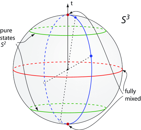
Figure 1: (colour online) Manifold of $2\times 2$ density matrices. The sphere $S^{3}$ of radius $1/\surd{2}$ constitutes the covering space for the space of $2\times 2$ density matrices. If we regard the $t$-axis as defining the ‘poles’, then the density matrix ${\hat{\varrho}}=\mbox{$\textstyle\frac{1}{2}$}{\mathds{1}}$ corresponds to the ‘north’ and the ‘south’ poles, as well as the equator. Moving down from the north pole, at $t=\pm\frac{1}{2}$ we have the latitudinal ‘circles’ $S^{2}$ given by $x^{2}+y^{2}+z^{2}=\mbox{$\textstyle\frac{1}{4}$}$, corresponding to the pure-state boundary. Crossing this boundary by further reducing the value of $t$ we see a ‘mirror image’, where starting from pure state one approaches the fully-mixed state ${\hat{\varrho}}=\mbox{$\textstyle\frac{1}{2}$}{\mathds{1}}$ as $t\to 0$. The northern hemisphere of the $S^{3}$ is thus partitioned into two parts; the northern cap $t\geq\frac{1}{2}$ and the latitudinal band $0\leq t<\frac{1}{2}$. Each point is identified with an antipodal point in the southern hemisphere, but in addition the points above and below $t=\frac{1}{2}$ are also identified in pairs; and finally, the equator is identified as a single point, also to be identified with the two poles.

As a concrete example, let us work out the variance lower bound associated with the estimation of unitary (e.g., time) parameter. The problem is as follows. We have a system prepared in an initial state ${\hat{\xi}}_{0}={\hat{\xi}}(0)$, which evolves under the Hamiltonian ${\hat{H}}$ so that

$${\hat{\xi}}_{t}=\exp(-\mbox{$\rm i$}{\hat{H}}t){\hat{\xi}}_{0}\exp(\mbox{$\rm i$}{\hat{H}}t).$$ (20)

The task is to estimate how much time has elapsed since its initial preparation. Let ${\hat{T}}$ be an unbiased estimator for the time parameter $t$ so that ${\rm tr}({\hat{T}}{\hat{\xi}}_{t}{\hat{\xi}}_{t})=t$ (strictly speaking, all we need is a locally unbiased estimator satisfying $\partial_{t}{\rm tr}({\hat{T}}{\hat{\xi}}_{t}{\hat{\xi}}_{t})=1$) Holevo . If we write ${\tilde{T}}={\hat{T}}-t{\mathds{1}}$ for the mean-adjusted estimator, then the variance of ${\hat{T}}$ is $\Delta T^{2}={\rm tr}({\tilde{T}}^{2}{\hat{\xi}}_{t}{\hat{\xi}}_{t})$. By differentiating the trace condition ${\rm tr}({\hat{\xi}}_{t}{\hat{\xi}}_{t})=1$ in $t$ and writing ${\hat{\xi}}^{\prime}_{t}=\partial_{t}{\hat{\xi}}_{t}$, we obtain ${\rm tr}({\hat{\xi}}^{\prime}_{t}{\hat{\xi}}_{t})=0$. Hence by differentiating ${\rm tr}({\tilde{T}}\xi_{t}\xi_{t})=0$ in $t$ and using ${\tilde{T}}^{\prime}=-{\mathds{1}}$ we find

$${\rm tr}[({\tilde{T}}{\hat{\xi}}_{t}+{\hat{\xi}}_{t}{\tilde{T}}){\hat{\xi}}^{\prime}_{t}]=1.$$ (21)

Recall that the matrix Schwarz inequality applied to a pair of Hermitian operators ${\hat{X}}$ and ${\hat{Y}}$ states that $[{\rm tr}({\hat{X}}{\hat{Y}})]^{2}\leq{\rm tr}({\hat{X}}^{2}){\rm tr}({\hat{Y}}^{2})$. Squaring (21) and substituting ${\hat{X}}={\tilde{T}}{\hat{\xi}}_{t}+{\hat{\xi}}_{t}{\tilde{T}}$ and ${\hat{Y}}={\hat{\xi}}^{\prime}_{t}$ in the Schwarz inequality, we deduce a version of the quantum Cramér-Rao inequality

$$\Delta T^{2}+\delta T^{2}\geq\frac{1}{2\,{\rm tr}({\hat{\xi}}^{\prime}_{t}{\hat{\xi}}^{\prime}_{t})},$$ (22)

where $\delta T^{2}={\rm tr}({\hat{T}}{\hat{\xi}}_{t}{\hat{T}}{\hat{\xi}}_{t})-t^{2}$, and where the denominator on the right side is half the Fisher-Rao metric. By use of the unitary evolution ${\hat{\xi}}^{\prime}_{t}=-\mbox{$\rm i$}({\hat{H}}{\hat{\xi}}_{t}-{\hat{\xi}}_{t}{\hat{H}})$ we find that

$${\rm tr}({\hat{\xi}}^{\prime}_{t}{\hat{\xi}}^{\prime}_{t})=2\left[{\rm tr}({\hat{H}}^{2}{\hat{\xi}}^{2}_{t})-{\rm tr}({\hat{H}}{\hat{\xi}}_{t}{\hat{H}}{\hat{\xi}}_{t})\right].$$ (23)

The right side of (23) is twice the skew information introduced by Wigner and Yanase WY . It is interesting that Fisher introduced the left side of (23), in the classical context, as the amount of extractable information concerning the value of $t$ Fisher , whereas Wigner and Yanase introduced the right side of (23), in the quantum context, as an a priori measure of information contained in the state concerning “not easily measured quantities” (such as ${\hat{T}}$) WY . In special cases for which ${\hat{\xi}}_{t}$ is a pure state satisfying ${\hat{\xi}}_{t}^{2}={\hat{\xi}}_{t}$, the skew information is maximised and (23) coincides with twice the energy variance $2\Delta H^{2}$, while $\delta T^{2}=0$, and we recover the uncertainty relation for the unitary parameter estimation as in Brody1 . For mixed states, however, we obtain

$$\Delta T^{2}+\delta T^{2}\geq\frac{1}{4(\Delta H^{2}-\delta H^{2})}.$$ (24)

We note that for an arbitrary observable ${\hat{H}}$ the Wigner-Yanase skew information $I_{\rho}$ is defined by the expression

$$I_{\rho}(H)={\rm tr}({\hat{H}}^{2}{\hat{\rho}})-{\rm tr}({\hat{H}}\sqrt{\hat{\rho}}{\hat{H}}\sqrt{\hat{\rho}}),$$ (25)

whereas the quantity $\delta H$ introduced above, which might appropriately be called the skew information of the second kind, is given by

$$\delta H^{2}={\rm tr}({\hat{H}}\sqrt{\hat{\rho}}{\hat{H}}\sqrt{\hat{\rho}})-\left[{\rm tr}({\hat{H}}{\hat{\rho}})\right]^{2}.$$ (26)

It follows that the total variance takes the form $\Delta H^{2}=I_{\rho}(H)+\delta H^{2}$, which can be interpreted as the quantum analogue of the conditional variance formula (that the total variance is the sum of the expectation of the conditional variance and the variance of the conditional expectation). In particular, it is easily shown that $\Delta T^{2}\geq\delta T^{2}\geq 0$. By taking the upper bound for $\delta T^{2}$, one obtains $\Delta T^{2}\geq 1/4\,{\rm tr}({\hat{\xi}}^{\prime}_{t}{\hat{\xi}}^{\prime}_{t})$, which is the uncertainty relation based on the skew information obtained by Luo Luo (see also Petz2 ). This bound is not tight because the Luo relation gives $\Delta T^{2}\Delta H^{2}\geq 1/8$ for pure states, whereas (22) gives $\Delta T^{2}\Delta H^{2}\geq 1/4$. If we combine (24) with its dual inequality $\Delta H^{2}+\delta H^{2}\geq 1/4(\Delta T^{2}-\delta T^{2})$, we obtain a less tight but more symmetric expression

$$\Delta T^{2}\Delta H^{2}\geq\mbox{$\textstyle\frac{1}{4}$}+\delta T^{2}\delta H^{2},$$ (27)

which implicitly appears in Luo2 .

By exploiting the utility of information geometry, we can go beyond the lowest-order term in uncertainty relations. To this end, we remark that the Fisher-Rao metric that determines the uncertainty lower bound is just the squared ‘velocity’ of the evolution of quantum states. In the case of a pure state, the fact that squared velocity of the state evolution is given by the energy uncertainty is known as the Anandan-Aharonov relation AA . The observation of Luo can be paraphrased by saying that this velocity, in the case of a generic mixed state, is given by the skew information. In addition to the squared velocity, we consider the squared ‘acceleration’ ${\hat{\alpha}}_{t}={\hat{\xi}}^{\prime\prime}_{t}-{\rm tr}({\hat{\xi}}^{\prime\prime}_{t}{\hat{\xi}}_{t}){\hat{\xi}}_{t}$, which determines the curvature $\gamma^{2}=16{\rm tr}({\hat{\alpha}}_{t}{\hat{\alpha}}_{t})/{\rm tr}({\hat{\xi}}^{\prime}_{t}{\hat{\xi}}^{\prime}_{t})$ of the curve in the space of square-root density matrices. The squared acceleration determines the next-order correction to the uncertainty relation. More generally, we can obtain arbitrarily many higher-order corrections by considering higher-order derivative terms, thus generalising the quantum Bhattacharrya bounds derived in Brody1 ; Brody2 ; Brody3 for pure states to general density matrices.

To illustrate how higher-order corrections to uncertainty relations can be obtained systematically, let us examine the second-order and the third-order corrections here. For this purpose, it will be convenient to relax the unit trace condition ${\rm tr}{\hat{\rho}}=1$ but merely require ${\rm tr}{\hat{\rho}}\neq 0$ and ${\rm tr}{\hat{\rho}}<\infty$, and impose unit trace at the end of the calculation. We then define the symmetric function $t({\hat{\xi}})={\rm tr}({\hat{\xi}}{\hat{T}}{\hat{\xi}})/{\rm tr}({\hat{\xi}}{\hat{\xi}})$ of ${\hat{\xi}}$ and consider the gradient $\nabla t$ of this function in the space of square-root density matrices, evaluated at ${\rm tr}({\hat{\xi}}{\hat{\xi}})=1$. A short calculation then shows that the squared magnitude (in the Hilbert-Schmidt norm) of the gradient is $|\nabla t|^{2}=2(\Delta T^{2}+\delta T^{2})$. On the other hand, the squared magnitude of the gradient is clearly larger than (or equal to) the squared magnitude of its component in the direction of ${\hat{\xi}}^{\prime}_{t}$, and thus $\Delta T^{2}+\delta T^{2}\geq 1/2{\rm tr}({\hat{\xi}}^{\prime}_{t}{\hat{\xi}}^{\prime}_{t})$, where we have made use of the relation ${\rm i}[{\hat{H}},{\hat{T}}]=1$. This provides an alternative derivation of the quantum Cramér-Rao inequality.

The next order correction to the uncertainty lower bound for mixed states is obtained from the component of $\nabla t$ in the direction of ${\hat{\alpha}}_{t}$, given by ${\rm tr}(({\hat{T}}{\hat{\xi}}_{t}+{\hat{\xi}}_{t}{\hat{T}}){\hat{\alpha}}_{t})/{\rm tr}({\hat{\alpha}}_{t}{\hat{\alpha}}_{t})$. Hence if the curvature $\gamma$ of the curve ${\hat{\xi}}_{t}$ is large, the correction is small. The numerator, however, in general depends on ${\hat{T}}$. To seek a bound that is independent of ${\hat{T}}$ we thus consider the third-order term, i.e. the component of the gradient in the direction of ${\hat{\beta}}_{t}={\hat{\xi}}_{t}^{\prime\prime\prime}-({\rm tr}({\hat{\xi}}_{t}^{\prime\prime\prime}{\hat{\xi}}_{t}^{\prime})/{\rm tr}({\hat{\xi}}_{t}^{\prime}{\hat{\xi}}_{t}^{\prime})){\hat{\xi}}_{t}^{\prime}$. This is given by ${\rm tr}(({\hat{T}}{\hat{\xi}}_{t}+{\hat{\xi}}_{t}{\hat{T}}){\hat{\beta}}_{t})/{\rm tr}({\hat{\beta}}_{t}{\hat{\beta}}_{t})$. Although the calculation of this term is straightforward, the resulting expression is lengthy and will be omitted here. It suffices to note that each of the odd-order corrections involves commutators between ${\hat{T}}$ and ${\hat{H}}^{k}$ for some $k$, and thus is independent of ${\hat{T}}$; whereas all even-order corrections are in general dependent on ${\hat{T}}$. Furthermore, terms appearing in the corrections have specific statistical interpretations in terms of the quantum extensions of central moments of the Hamiltonian. In the pure state limit where ${\hat{\xi}}_{t}^{2}={\hat{\xi}}_{t}$, these expressions reduce to the “classical” central moments, in a manner analogous to the reduction of the Wigner-Yanase skew information to the second central moment $\Delta H^{2}$. We are thus able to obtain various higher-order generalisations of the skew information, which appear to be entirely new quantities in the study of statistical properties of mixed states in quantum mechanics. These quantities might appropriately be called quantum skew moments.

I thank E. J. Brody, E. M. Graefe, L. P. Hughston, M. F. Parry, and the participants of the third international conference on Information Geometry and Its Applications, Leipzig 2010, for stimulating discussions.

References

- (1) Hübner, M. “Explicit computation of the Bures distance for density matrices” Phys. Lett. A163, 239 (1992).
- (2) Petz, D. and Sudár, C. “Geometry of quantum states” J. Math. Phys. 37, 2662 (1996).
- (3) Uhlmann, A. “Spheres and hemispheres as quantum state spaces” J. Geom. Phys. 18, 76 (1996).
- (4) Bengtsson, I. and Zyczkowski, K. Geometry of Quantum States: An Introduction to Quantum Entanglement (Cambridge: Cambridge University Press 2007).
- (5) Hansen, F. “Metric adjusted skew information” Proc. Nat. Acad. Sci. 105, 9909 (2008).
- (6) Rao, C. R. “Information and the accuracy attainable in the estimation of statistical parameters” Bull. Calcutta Math. Soc. 37, 81 (1945).
- (7) Amari, S. and Nagaoka, H. Methods of Information Geometry (Oxford: Oxford University Press 2000).
- (8) Brody, D. C. and Hook, D. W. “Information geometry in vapour-liquid equilibrium” J. Phys. A42, 023001 (2009).
- (9) Wigner, E. P. and Yanase, M. M. “Information contents of distributions” Proc. Nat. Acad. Sci. 49, 910 (1963).
- (10) Braunstein, S. L. and Caves, C. M. “Statistical distance and the geometry of quantum states” Phys. Rev. Lett. 72, 3439 (1994).
- (11) Fujiwara, A. and Nagaoka, H. “Quantum Fisher metric and estimation for pure state models” Phys. Lett. A201, 119 (1995).
- (12) Caianiello, E. R. and Guz, W. “Quantum Fisher metric and uncertainty relations” Phys. Lett. A126, 223 (1988).
- (13) Brody, D. C. and Hughston, L. H. “Geometry of quantum statistical inference” Phys. Rev. Lett. 77, 2851 (1996).
- (14) Luo, S. “Wigner-Yanase skew information and uncertainty relations” Phys. Rev. Lett. 91, 180403 (2003).
- (15) Luo, S. “Logarithm versus square root: Comparing quantum Fisher information” Commun. Theo. Phys. 47, 597 (2007).
- (16) Gibbons, G. W. “Typical states and density matrices” J. Geom. Phys. 8, 147 (1992).
- (17) A. S. Holevo, Probabilistic and Statistical Aspects of Quantum Theory (North-Holland Publishing Company, Amsterdam, 1982).
- (18) Fisher, R. A. “Theory of statistical estimation” Proc. Camb. Phil. Soc. 22, 700 (1925).
- (19) Gibilisco, P., Hiai, F. and Petz, D. Covariance, quantum Fisher information, and the uncertainty relations IEEE Trans. Inf. Theory 55, 439 (2009).
- (20) Luo, S. “Heisenberg uncertainty relation for mixed states” Phys. Rev. A72, 042110 (2005).
- (21) Anandan, J. and Aharonov, Y. “Geometry of quantum evolution” Phys. Rev. Lett. 65, 1697 (1990).
- (22) Brody, D. C. and Hughston, L. H. “Generalised Heisenberg relations for quantum statistical estimation” Phys. Lett. A236, 257 (1997).
- (23) Brody, D. C. and Hughston, L. H. “Statistical geometry in quantum mechanics” Proc. R. Soc. London A454, 2445 (1998).