An Atlas of $z=5.7$ and $z=6.5$ Ly$\alpha$ Emitters

Abstract

We present an atlas of 88 $z\sim 5.7$ and 30 $z\sim 6.5$ Ly$\alpha$ emitters obtained from a wide-field narrowband survey. We combined deep narrowband imaging in 120 Å bandpass filters centered at 8150 Å and 9140 Å with deep $BVRIz$ broadband imaging to select high-redshift galaxy candidates over an area of 4180 arcmin². The goal was to obtain a uniform selection of comparable depth over the 7 targeted fields in the two filters. For the GOODS-N region of the HDF-N field, we also selected candidates using a 120 Å filter centered at 9210 Å. We made spectroscopic observations with Keck DEIMOS of nearly all the candidates to obtain the final sample of Ly$\alpha$ emitters. At the 3.3 Å resolution of the DEIMOS observations the asymmetric profile for Ly$\alpha$ emission can be clearly seen in the spectra of nearly all the galaxies. We show that the spectral profiles are surprisingly similar for many of the galaxies and that the composite spectral profiles are nearly identical at $z=5.7$ and $z=6.5$. We analyze the distributions of line widths and Ly$\alpha$ equivalent widths and find that the lines are marginally narrower at the higher redshift, with median values of $0.77$ Å at $z=6.5$ and $0.92$ Å at $z=5.7$. The line widths have a dependence on the Ly$\alpha$ luminosity of the form $\sim L_{\alpha}^{0.3}$. We compare the surface densities and the luminosity functions at the two redshifts and find that there is a multiplicative factor of 2 decrease in the number density of bright Ly$\alpha$ emitters from $z=5.7$ to $z=6.5$, while the characteristic luminosity is unchanged.

1. Introduction

Table 1Narrowband Survey Fields

Field	R.A.	Decl.	($l^{\rm{II}},b^{\rm{II}}$)	EB-V	NB816	NB912
	(J2000)	(J2000)			(hrs)	(hrs)
SSA22	22:17:57.00	+00:14:54.5	(63.1,$-44.1$)	0.07	3.8	8.4
SSA22_new	22:18:24.67	+00:36:53.4	(63.6,$-43.9$)	0.06	4.8	9.0
A370	02:39:53.00	$-$01:34:35.0	(173.0,$-53.6$)	0.03	4.6	7.9
A370_new	02:41:16.27	$-$01:34:25.1	(173.4,$-53.3$)	0.03	4.6	8.0
HDF-N	12:36:49.57	+62:12:54.0	(125.9,$+54.8$)	0.01	9.7	8.3
HDF-N_new	12:40:26.40	+62:21:45.0	(125.1,$+54.7$)	0.01	7.1	10.0
SSA17	17:06:36.22	+43:55:39.5	(69.1,$+36.8$)	0.02	5.1	4.5

Ever since the first discovery of Ly$\alpha$ emitters above redshift $z\sim 6$ (Hu et al. 2002), the goal has been to identify substantial samples of high-redshift Ly$\alpha$ emitters in order to study such diverse topics as the formation of galaxies in the early universe, early structure formation, reionization, and the interactions of galaxies with the intergalactic medium (IGM). The advent of deep, wide-field, narrowband surveys (e.g., Hu et al. 2004; hereafter, H04; Wang et al. 2005; Shimasaku et al. 2006; Kashikawa et al. 2006; Ouchi et al. 2008) has recently made it possible to obtain substantial numbers of galaxies at $z\sim 5.7$ and $z\sim 6.5$, where gaps in the night sky emission permit deep studies, for addressing these topics. However, the straightforward interpretation of these survey results has been plagued by statistical and cosmic variance from field to field (e.g., Hu & Cowie 2006) and by the absence of extensive spectroscopic follow-up of the primarily photometrically selected samples. As we shall show in the present work, photometric samples can have a substantial degree of contamination, and spectroscopy is necessary to remove these interlopers. With high-resolution spectroscopic follow-ups of the candidates, it is possible both to confirm that the emission is due to redshifted Ly$\alpha$ and to estimate the statistics of interlopers.

Here we present the results of a wide-field, narrowband survey with highly complete spectroscopic follow-up. We used the $34^{\prime}\times 27^{\prime}$ field-of-view SuprimeCam mosaic CCD camera (Miyazaki et al. 2002) on the Subaru 8.2 m telescope to observe seven different target fields to search for Ly$\alpha$ emitters at $z\sim 5.7$ (NB816) and $z\sim 6.5$ (NB912, NB921). In Section 2 we summarize the narrowband and continuum imaging together with the candidate selection. The data obtained in these narrowbands are comparable in depth, and we have analyzed them with uniform selection and processing criteria. We have spectroscopically observed nearly all the photometrically selected objects with the DEep Imaging Multi-Object Spectrograph (DEIMOS; Faber et al. 2003) on the Keck II 10 m telescope, which we also describe in Section 2.

The resulting photometric and spectroscopic samples form a large, consistent data set with which to tackle the cosmological problems. We provide spectra for 88 $z\sim 5.7$ and 30 $z\sim 6.5$ Ly$\alpha$ emitting galaxies. This forms the largest sample of confirmed high-redshift galaxies in the very distant universe. We give the catalogs, thumbnail images, and spectra in the Appendix.

In Section 3 we discuss the relative properties of the samples at $z=5.7$ and $z=6.5$. The emission-line properties provided by the spectra are key diagnostics of the intergalactic gas properties at these redshifts. They may be used to probe the neutral fraction of the surrounding intergalactic medium (IGM; e.g., Gnedin & Prada 2004; Santos 2004; Zheng et al. 2010) and thus to study the ionization state of the IGM and its redshift evolution at early times. Theoretical models make predictions of the impact of the neutral portion of the IGM on the line profile of Ly$\alpha$ emission and also upon the redshift evolution of the Ly$\alpha$ luminosity function (e.g., Barkana & Loeb 2001; Mesinger & Furlanetto 2004; Dijkstra et al. 2007; Dijkstra & Wyithe 2010). In Section 3 we analyze the line width distributions at $z=5.7$ and $z=6.5$, showing that there are only small changes in the properties of the lines over this range and that the line properties are remarkably similar for most of the objects. We find that there is a dependence of line width on Ly$\alpha$ luminosity, with the more luminous objects being broader. We show that the luminosity function (LF) drops by a factor of two at $z=6.5$ relative to that at $z=5.7$, and the $z=5.7$ value is a factor of four lower than that at $z=3.1$. However, the characteristic luminosity is unchanged. The results are for the observed luminosities, and the fall-off will be less for the intrinsic LFs when the effects of intergalactic scattering are allowed for.

In a subsequent paper we will combine the optical data with longer wavelength observations from the Hubble Space Telescope (HST) and discuss the UV continuum properties of the high-redshift sample and the Ly$\alpha$ escape fraction.

We assume $\Omega_{M}=0.3$, $\Omega_{\Lambda}=0.7$, and $H_{0}=70$ km s^-1 Mpc^-1 throughout. All magnitudes are given in the AB magnitude system (Oke et al. 1983, 1990), where an AB magnitude is defined by $m_{AB}=-2.5\log f_{\nu}-48.60$. Here $f_{\nu}$ is the flux of the source in units of erg cm^-2 s^-1 Hz^-1.

2. Narrowband Selection

2.1. Observed Fields

The present survey covers seven SuprimeCam fields. We summarize these in Table 1, where we give the name of the field in column 1, the J2000 right ascension and declination of the field centers in columns 2 and 3, the galactic longtitude and latitude in column 4, the galactic extinction to the field in column 5, and the exposure times in hours through the NB816 and NB912 filters in columns 6 and 7. The field geometry is shown in Figure 1. Six of the fields are grouped into three neighboring and slightly overlapping pairs to allow a study of clustering. The seventh field (SSA17) is isolated. The very central region of the A370 field is lensed by the foreground massive cluster A370 at $z=0.37$.

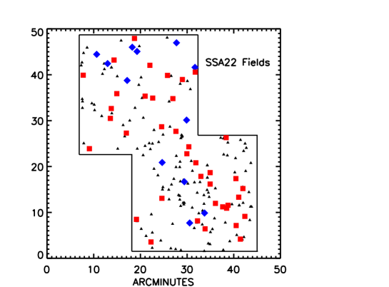
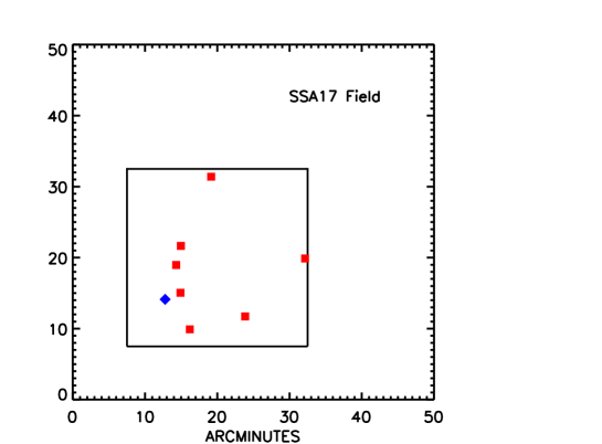
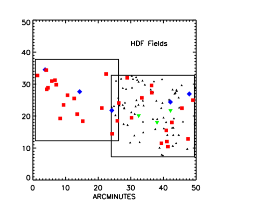
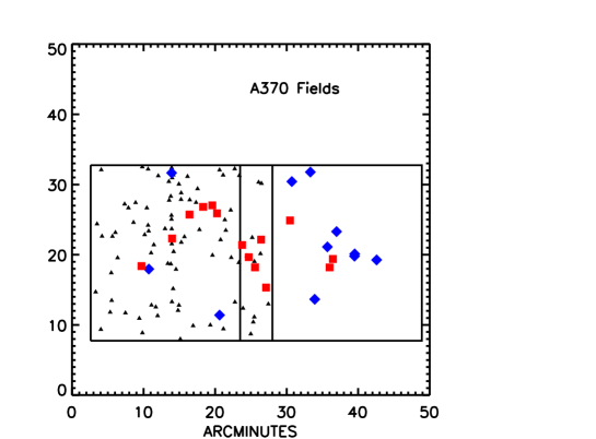
Figure 1.— The geometric configurations of the seven SuprimeCam fields. Six of the fields are grouped into pairs with small amounts of overlap, while one is isolated (SSA17). The solid lines outline the observed areas. The red squares show the detected Ly$\alpha$ emitters at $z\sim 5.7$, the blue diamonds show those at $z\sim 6.5$, and the green downward pointing triangles show sources found using the 9210 Å filter (GOODS-N only). Four of the fields were used in the Kakazu et al. (2007) survey of $z<1.6$ ultra-strong emission-line galaxies. These objects are denoted by black small triangles.

We obtained the narrowband images of each field with SuprimeCam under photometric or near-photometric conditions. We observed each field with a 120 Å (FWHM) filter (NB816) centered at a nominal wavelength of 8150 Å corresponding to a $z\sim 5.7$ selection and a 120 Å (FWHM) filter (NB912) centered at a nominal wavelength of 9140 Å corresponding to a $z\sim 6.5$ selection. Both lie in regions of low sky background between the OH bands. (The nominal specifications for the Subaru filters may be found at www.naoj.org/Observing/Instruments/SCam/sensitivity.html and are described in Ajiki et al. 2003.) We show the location and shape of both filter profiles in Figure 2(a). We also show the wavelength positions of all the spectroscopically confirmed $z\sim 5.7$ Ly$\alpha$ emitters (red squares) and $z\sim 6.5$ Ly$\alpha$ emitters (blue diamonds) in all seven fields. The Gaussian shape of the SuprimeCam filter profiles may be compared with the more square profile of the 108 Å filter centered at 8185 Å that has been used in the Low-Resolution Imaging Spectrograph (LRIS; Oke et al. 1995) parallel beam on Keck I (Hu et al. 1999). The complex shape of the SuprimeCam filter profiles requires careful treatments of the conversion of narrowband magnitudes to line fluxes and of the determination of the accessible volume (e.g., Gronwall et al. 2007). We carry this out in Section 3.

The NB816 filter is well centered on the Cousins $I$-band filter, which we use as the reference continuum bandpass for the $z\sim 5.7$ selection. The NB912 filter is well centered on the $z$-band, which we use as the reference continuum bandpass for the $z\sim 6.5$ selection. For the Great Observatories Origins Deep Survey-North (GOODS-N; Giavalisco et al. 2004) region of the Hubble Deep Field-North (HDF-N), we also selected objects using a 120 Å filter centered at 9210 Å. We show this filter profile (green) in Figure 2(b), along with the other two filter profiles from Figure 2(a). We show the wavelength positions of all the spectroscopically confirmed $z\sim 6.5$ Ly$\alpha$ emitters found with this filter (green triangles; 3 objects), along with the positions of the spectroscopically confirmed $z\sim 5.7$ Ly$\alpha$ emitters found with the NB816 filter in this field (red squares; 5 objects). No $z\sim 6.5$ Ly$\alpha$ emitters were found in the GOODS-N with the NB912 filter.

Table 1 summarizes the observations made in the primary bands, including giving the total photometric exposure time in hours for each of the filters in each of the fields. We obtained $\sim 4-5$ hour exposures for the NB816 filter and $\sim 8-10$ hour exposures for the NB912 filter. The longer exposures in the NB912 filter partially compensate for the lower camera throughput at this wavelength, so the observations provide comparable depth exposures in the two bands. However, the NB912 images are still slightly shallower than those in the NB816 band. We took the data as a sequence of dithered background-limited exposures with alternate sequences rotated by 90 deg. We always obtained the corresponding continuum exposures in the same observing run as the narrowband exposures to avoid falsely identifying transients—such as high-redshift supernovae or Kuiper belt objects—as Ly$\alpha$ candidates. Capak et al. (2004) gives a detailed description of the full reduction procedure that we used to process the images. We calibrated the SuprimeCam data using photometric and spectrophotometric standard stars (Turnshek et al. 1990; Oke et al. 1990) and faint Landolt standard stars (Landolt et al. 1992). We obtained an astrometric solution using stars from the USNO survey. The final narrowband selected samples were drawn from the more uniformly covered central $25^{\prime}\times 25^{\prime}$ region of each of the fields. Allowing for overlaps, the combined area of the 7 fields in the survey is 4168 arcmin². We note that the present calibration of the SSA22 field is about 0.2 mag fainter than that given in H04. This is typical of the errors introduced in the calibrations and in the choice of method for measuring the magnitudes. Thus, we adopt it as an estimate of the systematic error in the absolute measurements. The relative magnitudes are extremely well determined in the field compared to the absolute calibration, so the relative counts and LFs in the NB912 and NB816 bands are insensitive to this issue. However, it does affect the normalization of the LF. The FWHM seeing on the final reduced images ranges from $0.5^{\prime\prime}$ to $1^{\prime\prime}$. The typical limiting magnitudes of the images ($5\sigma$ for the corrected $3^{\prime\prime}$ diamteer aperture mags, see Section 2.2) expressed as AB magnitudes are 26.9 ($B$), 26.8 ($V$), 26.6 ($R$), 25.6 ($I$), 25.4 ($z$), 25.3 (NB816), and 25.2 (NB912), though the exact values vary slightly depending on the exposure time and the observing conditions.

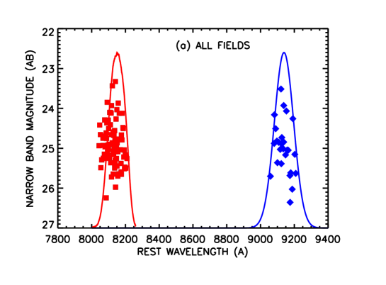
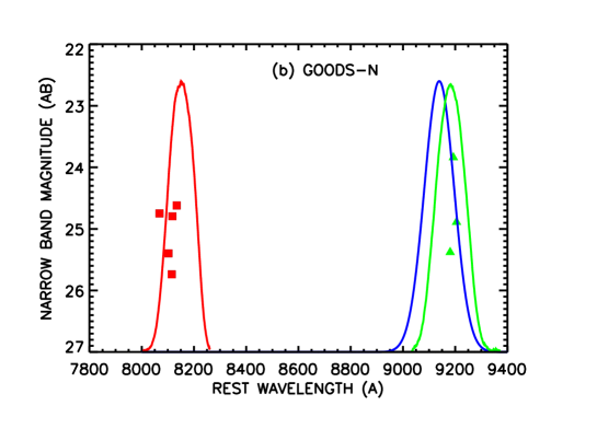
Figure 2.— (a) The transmission profiles versus rest-frame wavelength for the two primary filters (NB816/8150 Å in red and NB912/9140 Å in blue). We also show the wavelength positions of all the spectroscopically confirmed $z\sim 5.7$ Ly$\alpha$ emitters (red squares) and $z\sim 6.5$ Ly$\alpha$ emitters (blue diamonds) in the fields. (b) The transmission profiles from (a) plus the transmission profile of the 9210 Å filter (green) used in the GOODS-N region of the HDF-N field. We also show the wavelength positions of all the spectroscopically confirmed $z\sim 6.5$ Ly$\alpha$ emitters found with this filter (green triangles; 3 objects), along with the spectroscopically confirmed $z\sim 5.7$ Ly$\alpha$ emitters found with the NB816 filter (red squares; 5 objects) in this field. No $z\sim 6.5$ Ly$\alpha$ emitters were found in the GOODS-N with the NB912 filter.

2.2. Photometric Candidate Selection

We used the SExtractor package (Bertin & Arnouts 1996) to generate catalogs of objects in each of the fields. We measured all of the magnitudes in $3^{\prime\prime}$ diameter apertures and applied average aperture corrections to obtain total magnitudes. The typical correction is just under 0.2 mags. (Hereafter, we refer to these as corrected $3^{\prime\prime}$ diameter aperture magnitudes.) Throughout the paper a negative sign in front of a magnitude means that the flux in the aperture was negative. The numerical value of the magnitude then corresponds to the absolute value of the flux. We follow this procedure so that the tables may be used to properly average fluxes including negative values.

In Figure 3 we show our measured number counts in the (a) NB816 and (b) NB912 bands (black squares). We have plotted the $1\sigma$ error bars, but they are generally smaller than the symbol size. These counts are averaged over all fields, with the exception of the A370 field, where lensing effects from the massive cluster may be important. In (a) we show a power-law fit to the NB816 counts (black line), which we compare with a power-law fit to the incompleteness corrected NB816 counts of Ouchi et al. (2008; their Figure 11) (blue line). The shapes of the counts are in extremely good agreement, but the normalization is slightly higher in our counts. This corresponds to our magnitudes being about 0.2 mag brighter, on average, than those of Ouchi et al. (2008). This again suggests that 0.2 mag is the level of uncertainty arising from the calibrations and from the magnitude measurements. All of our fields give consistent counts, and all show the same offset. By comparing the actual counts with the power-law fit, we see that our sample is highly complete to magnitudes just above NB816 $=25.5$.

We do not have a previous comparison for the NB912 sample, so in Figure 3(b) we compare with the F850LP selected number counts from the HST ACS observations of the GOODS fields (Giavalisco et al. 2004) (red open diamonds). The F850LP filter has a very similar color response to the $z$ filter, which we use as the continuum for the NB912 filter. Thus, it should provide a good approximation to the NB912 counts. Indeed, the HST counts agree closely with the NB912 counts. We used these much deeper counts to determine the form of the power-law fit, and then we renormalized the fit to match the bright-end counts in the NB912 band. We show this fit as the blue line in Figure 3(b). We see that the NB912 counts become progressively incomplete above NB912 $\sim 25$. We use the ratio of this power-law fit to the observed counts to calculate an incompleteness correction as a function of the NB912 magnitude. For the NB816 band we compute the incompleteness correction using the power-law fit to Ouchi et al. (2008)’s incompleteness corrected counts. At NB912 $=25.5$ the correction is a multiplicative factor of 2.3, while at NB816 $=26.0$ the correction is 2.0.

For each field we formed a sample of galaxies with narrowband magnitudes $N_{\rm AB}<25.5$ satisfying either the criterion $(I-N)_{\rm AB}>0.8$ in the NB816 band or $(z-N)_{\rm AB}>0.9$ in the NB912 band. Following Kakazu et al. (2007), we refer to these objects as ultra-strong emission-line galaxies or USELs. Our narrowband excess selection criteria are slightly lower than those used by Ouchi et al. (2008) [$(i^{\prime}-$NB816)$>1.2$] or by Taniguchi et al. (2005) [$(z-$NB921)$>1$]. These groups wanted to choose more securely genuine emission-line galaxies in their photometric samples, while we seek completeness and rely on the subsequent spectroscopic observations to eliminate false objects where the narrowband excess is not produced by an emission line lying in the filter bandpass.

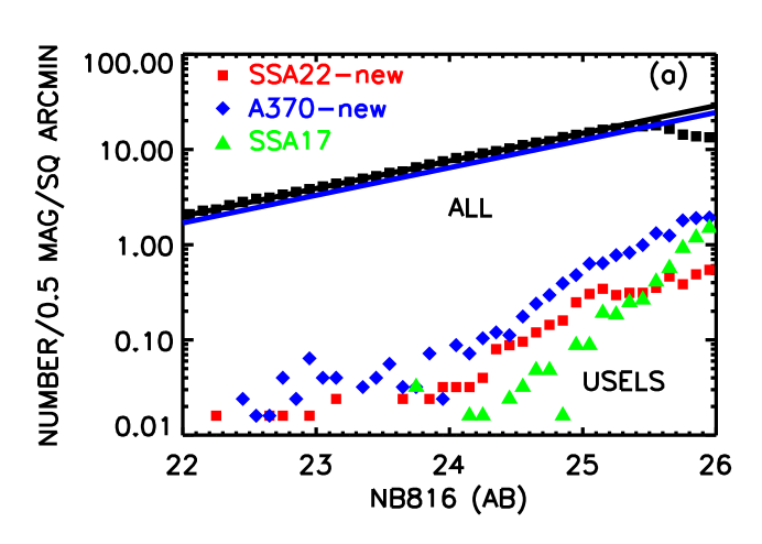
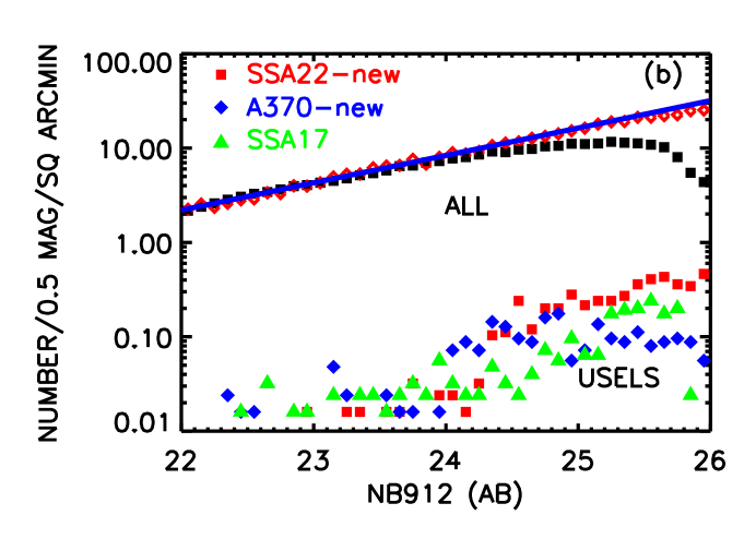
Figure 3.— Measured number counts of narrowband selected objects in the (a) NB816 and (b) NB912 bands (black squares). A power-law fit to the NB816 number counts [black line in (a)] may be compared with a power-law fit to the incompleteness corrected number counts measured in this band by Ouchi et al. (2008) [blue line in (a)]. The NB912 number counts may be compared with the expected incompleteness corrected counts in this band determined from the HST ACS GOODS F850LP selected number counts [red open diamonds in (b)], which we fitted with a power law and then renormalized to match the bright-end counts in the NB912 band [blue line in (b)]. For three of the fields we also show the number density of USEL candidates (see figure legends).

We visually inspected each USEL candidate to eliminate artifacts, and we also visually searched the images for USELs that might have been missed in the initial catalog because they were blended with neighboring objects. In Figure 4 we show examples of the final USEL selection. In (a) we show $(I-N)_{\rm AB}$ versus $N_{\rm AB}$ for the NB816 selected objects in the SSA22$\_$new field, and in (c) we show $(z-N)_{\rm AB}$ versus $N_{\rm AB}$ for the NB912 selected objects in the SSA22$\_$new field. The small symbols show the entire sample of $N_{\rm AB}<25.5$ galaxies in the field. The blue horizontal line shows the narrowband color selection. Objects satisfying these criteria are shown with large symbols. As can be seen from the figures, this sample will include a number of objects at the faint end that have scattered into the selection region. Thus, as mentioned above, with this approach we rely on the subsequent spectroscopic observations to eliminate any spurious objects. For the NB816 selected sample in the SSA22$\_$new field we find 101 objects with $(I-N)_{\rm AB}>0.8$ over the $25^{\prime}\times 25^{\prime}$ field, which is about 0.3% of the 36816 objects included in the initial $N_{\rm AB}<25.5$ sample. For the NB912 selected sample in this field we find 183 USEL candidates, which is about 0.5% of the 38120 objects. We show the number density of USEL candidates versus narrowband magnitude for three of the individual fields in Figure 3. All the fields have similar number densities of USEL candidates, which rise rapidly to fainter magnitudes.

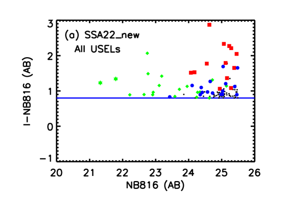
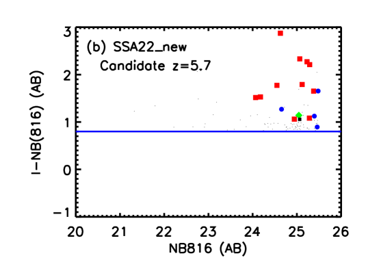
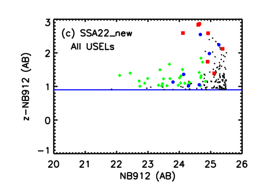
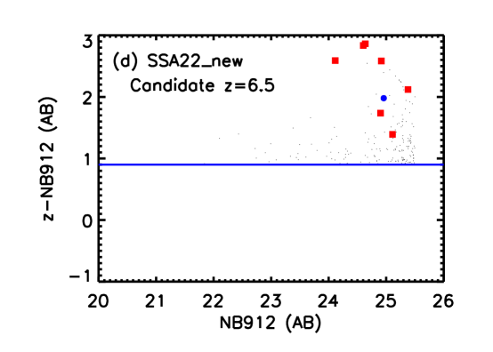
Figure 4.— Emission-line excess objects found using (a) the NB816 filter in the SSA22$\_$new field and (c) the NB912 filter in the SSA22$\_$new field vs. $N_{\rm AB}$ magnitude. The small symbols show the entire sample of $N_{\rm AB}<25.5$ galaxies in the field. The blue horizontal line shows the narrowband excess selection of (a) $(I-N)_{\rm AB}>0.8$ for NB816 and (c) $(z-N)_{\rm AB}>0.9$ for NB912. Objects satisfying these criteria are shown with large symbols: green diamonds—spectroscopically classified low-redshift emitters ($z<1.6$); green stars—spectroscopically classified stars; red squares—spectroscopically confirmed $z\sim 5.7$ emitters or $z\sim 6.5$ emitters; blue circles—spectroscopically observed but unidentified objects; black squares—objects with no spectroscopic measurements. (b) and (d) are similar to (a) and (c) but the large symbols are restricted to either objects with a strong break between the $R$- and $z$-bands ($I$- and $z$-bands) for NB816 (NB912) or objects which are undetected at the $2\sigma$ level in the $R$-band ($I$-band) for NB816 (NB912) and which are not detected in the $B$- or $V$- (or $R$-) bands. [Because of space constraints only points satisfying the narrowband excess selection are shown in this version of the paper]

We next eliminated USELs whose continuum colors rule them out as candidate $z\sim 5.7$ or $z\sim 6.5$ galaxies. For $z=5.7$ we restricted either to objects with $(R-z)_{\rm AB}>1.5$ or to objects which were not detected at the $2\sigma$ level in the $R$-band. We also required that the objects not be detected above the $2\sigma$ level in the $B$- and $V$-bands. For $z\sim 6.5$ we restricted either to objects with $(I-z)_{\rm AB}>1.5$ or to objects which were not detected at the $2\sigma$ level in the $I$-band. We also required that the objects not be detected above the $2\sigma$ level in the $B$-, $V$- and $R$-bands. The results from these restrictions on the USEL sample are shown in Figures 4(b) and (d) with the large symbols. We call these objects $z=5.7$ and $z=6.5$ candidate Ly$\alpha$ emitters, and we made an effort to obtain spectra of all of them. Typically, there are $\sim 20$ candidates in each field at $z\sim 5.7$ and $\sim 10$ at $z\sim 6.5$. In four of the fields (A370_new, HDF-N, SSA22, and SSA22_new; see Figure 1) we obtained spectra of all of the USELs with $N_{\rm AB}<24$ and many of the USELs with $N_{\rm AB}=24-25$, regardless of their colors. These results are described in Kakazu et al. (2007) and Hu et al. (2009).

As can be seen from Figures 4(b) and 4(d), the number of candidates is not particularly sensitive to the choice of narrowband excess. If we had used the Ouchi et al. (2008) cut of 1.2 in Figure 4(b), then it would have eliminated 6 of the 17 candidate $z=5.7$ galaxies. Five of the eliminated candidates have been spectroscopically observed: two are spurious, one is a low-redshift emitter, and two are genuine $z=5.7$ emitters. Thus, using the higher cut slightly improves the accuracy of the selection but at the expense of losing some $z=5.7$ emitters. If we had used the Taniguchi et al. (2005) cut of 1.0 in Figure 4(d), then it would not have changed the candidate selection at all.

2.3. Spectroscopic Confirmation

Spectroscopic followup of the candidates is essential to rule out contaminants in the photometric selection. These can include lower redshift emission line galaxies, red galaxies or stars, transients and artifacts in the data. The spectroscy also provides precise redshifts which allow us to make an accurate determination of the line fluxes as well as providing us with the shapes and widths of the Ly$\alpha$ lines.

We used the DEIMOS spectrograph on the Keck II 10 m telescope for our spectroscopic follow-up of the candidate $z\sim 5.7$ and $z\sim 6.5$ Ly$\alpha$ emitters. For most of the observations we used the G830 $\ell$/mm grating blazed at 8640 Å with $1^{\prime\prime}$ wide slitlets because of its high resolution and excellent red sensitivity. In a small number of cases we used the slightly lower resolution G600 $\ell$/mm grating. Both configurations have sufficient resolution (e.g., 3.3 Å with G830 $\ell$/mm) to distinguish the $z\sim 1.19$ [O II] doublet structure from the profile of redshifted Ly$\alpha$ emission (see Figure 2 of H04). Redshifted [O III] emitters ($z\sim 0.62$) show up frequently as emission-line objects in the narrowband and can easily be identified by the doublet signature. The observed wavelength coverage is $\sim 3840$ Å with a typical range of $\sim 5900-9700$ Å. It generally encompasses redshifted H$\beta$ and [O III] lines in cases where the detected emission line might be H$\alpha$ at $z\sim 0.24$. This is particularly useful for dealing with the problematic instance of extragalactic H II regions with strongly suppressed [N II]. The G830 $\ell$/mm grating used with the OG550 $\ell$/mm blocker gives a throughput greater than 20% for most of this range and $\sim 28\%$ at 8150 Å.

We made the observations during a number of runs in the $2005-2010$ period. Just over 90% of the candidates were observed in each of the bands. We apply a spectroscopic incompleteness correction to allow for the missing fraction in the analysis of the LFs in Section 3. Exposure times ranged from one to six hours for each object.

We filled the DEIMOS masks with color-selected and magnitude-selected samples, which will be described elsewhere. All of the spectra (emission-line objects and field objects) were spectroscopically classified without reference to either their narrowband strengths or their color properties to avoid any subjective biasing of the line interpretation. We classified each candidate object as either a confirmed high-redshift emitter, a low-redshift emitter, a red star, or a false emission-line object (i.e., when the observed narrowband excess does not appear to correspond to an emission line). For each high-redshift emitter the redshift is measured at the peak of the emission line. Slightly more than half of the $z=5.7$ candidate Ly$\alpha$ emitters were spectroscopically confirmed. The fraction of confirmation for the $z=6.5$ candidate Ly$\alpha$ emitters is higher, but there is still a substantial degree of contamination.

2.4. GOODS-N

We summarize the results for objects in the GOODS-N in Tables 2 (NB816) and 3 (NB921). The GOODS-N comprises about a quarter of the HDF-N field and has the advantage of having extremely deep broadband images from the HST ACS imaging (Giavalisco et al. 2004). In addition, Ajiki et al. (2006) carried out an independent analysis using the NB816 data obtained in the present program in combination with the ACS data to identify candidate $z=5.7$ Ly$\alpha$ emitters in the field. Since the Ajiki et al. analysis is based on their reductions of the SuprimeCam images and uses different calibrations and magnitude measurements, it provides an excellent check on the present work.

We identified 12 candidate $z=5.7$ Ly$\alpha$ emitters in the NB816 band in the GOODS-N. We summarize their properties in Table 2, where we give the object number in column 1, the R.A.(J2000) and Decl.(J2000) in decimal degrees in columns 2 and 3, the NB816 magnitude in column 4, the $I-$NB816 color in column 5, the SExtractor auto magnitudes for the four ACS bandpasses taken from the ACS catalogs in columns 6-9, and the measured redshift in column 10. While the selection of the present candidates was made solely using the ground-based observations, all of the objects are contained in the ACS catalogs, and all have colors in the ACS observations that are consistent with their being $z\sim 5.7$ galaxies.

All of the objects were spectroscopically observed with exposures ranging from 1 to 6 hours. Where an object was spectroscopically confirmed as a $z\sim 5.7$ emitter, we give the redshift of the source in Table 2. Of the 12 candidates, we identified 6 as Ly$\alpha$ emitters. Some of the remaining cases may be genuine emitters that we have failed to identify with the spectra. However, for many of the unidentified objects, we have obtained multiple repeated spectra and have failed to find an emission line. One object appears to be a portion of a larger galaxy, where the photometry may be contaminated. Some of the remaining objects could be red stars or objects at high redshift whose continuum break is just below the narrowband filter, simulating an emission-line object. Other cases may simply be spurious detections. This is representative of the fields in general.

Ajiki et al. (2006) used a more restricted area of the GOODS-N and found 10 candidate $z\sim 5.7$ Ly$\alpha$ emitters. Eight of these overlap with the present sample. Their narrowband magnitudes show an average of $-0.1$ mag offsets and a spread of up to 0.3 mag relative to the present values, probably reflecting the different apertures used. We spectroscopically observed one of the two objects from the Ajiki et al. sample that did not overlap with ours, but we did not confirm it as a $z=5.7$ Ly$\alpha$ emitter. All of the confirmed $z=5.7$ Ly$\alpha$ emitters in the area used by Ajiki et al. are common to the two samples. In both samples we have confirmed spectroscopically half of the candidate emitters.

We did not find any candidate $z\sim 6.5$ Ly$\alpha$ emitters in the NB912 band in the GOODS-N. However, a deep 12.7 hr exposure that we obtained with a 120 Å narrowband filter at 9210 Å yielded four candidates. We summarize their properties in Table 3. We spectroscopically observed three of the four candidates and confirmed all of them as $z\sim 6.5$ Ly$\alpha$ emitters. Their redshifts place them at wavelengths where the NB912 filter is becoming insensitive (see Figure 2), so they are not picked out in the NB912 observations. One of the objects is extremely luminous (HC123725+621227) and has a very high S/N spectrum (see Figure A6). This object is very faint in the continuum, and it is not detected in the GOODS-N ACS catalogs. In contrast to the NB816 sample, where all of the objects are detected in the ACS F850LP filter, only two of the four objects are present in the ACS F850LP catalog. This reflects the fading in the magnitude produced by the continuum break at the Ly$\alpha$ line, which lies near the middle of the F850LP bandpass.

Table 2GOODS-N: NB816 Selected $z\sim 5.7$ Ly$\alpha$ Emitter Candidates

Number	R.A.	Decl.	$N_{\rm AB}$	$(I-N)_{\rm AB}$	F850LP	F775W	F606W	F435W	Redshift
	(J2000)	(J2000)
(1)	(2)	(3)	(4)	(5)	(6)	(7)	(8)	(9)	(10)
1	189.215240	62.32683	$24.51$	$1.049$	$26.89$	$27.66$	$29.16$	$\cdots$	5.675
2	189.216751	62.36460	$24.60$	$2.032$	$26.37$	$27.21$	$\cdots$	$28.56$	5.689
3	189.056106	62.12994	$24.68$	$1.133$	$25.99$	$26.61$	$28.35$	$28.49$	5.635
4	189.254120	62.35397	$24.86$	$0.8972$	$26.32$	$27.59$	$29.22$	$34.04$	$\cdots$
5	189.399750	62.23944	$24.88$	$1.642$	$26.06$	$26.56$	$28.90$	$27.67$	$\cdots$
6	189.324677	62.29974	$25.06$	$2.342$	$26.52$	$27.30$	$28.45$	$\cdots$	5.663
7	189.033004	62.14394	$25.08$	$1.853$	$26.36$	$26.57$	$29.44$	$\cdots$	5.640
8	189.456543	62.22942	$25.18$	$0.8409$	$24.56$	$25.93$	$29.52$	$\cdots$	$\cdots$
9	189.342285	62.26277	$25.43$	$1.387$	$25.55$	$26.70$	$31.33$	$\cdots$	$\cdots$
10	189.045471	62.17144	$25.49$	$2.116$	$26.54$	$27.13$	$\cdots$	$30.56$	5.673
11	189.366013	62.19613	$25.51$	$2.557$	$26.72$	$27.26$	$\cdots$	$\cdots$	$\cdots$
12	189.320419	62.23344	$25.67$	$1.265$	$25.60$	$26.47$	$\cdots$	$29.81$	$\cdots$

Table 3GOODS-N: NB921 Selected $z\sim 6.5$ Ly$\alpha$ Emitter Candidates

Number	R.A.	Decl.	$N_{\rm AB}$	$(z-N)_{\rm AB}$	F850LP	F775W	F606W	F435W	Redshift
	(J2000)	(J2000)
(1)	(2)	(3)	(4)	(5)	(6)	(7)	(8)	(9)	(10)
1	189.358170	62.20769	$23.68$	$9.472$	$\cdots$	$\cdots$	$\cdots$	$\cdots$	6.559
2	189.356873	62.29541	$24.36$	$2.016$	$26.38$	$\cdots$	$\cdots$	$\cdots$	no obs
3	189.093689	62.23458	$25.30$	$3.476$	$27.16$	$31.87$	$\cdots$	$\cdots$	6.560
4	189.157135	62.17277	$25.86$	$1.092$	$\cdots$	$\cdots$	$\cdots$	$\cdots$	6.546

2.5. Atlas of the $z=5.7$ and $z=6.5$ Ly$\alpha$ Emitters

Our final spectroscopically confirmed sample consists of 87 $z=5.7$ Ly$\alpha$ emitters found with the NB816 filter, 27 $z=6.5$ Ly$\alpha$ emitters found with the NB912 filter, and 3 $z=6.5$ Ly$\alpha$ emitters found with the 9210 Å filter in the GOODS-N only. We include in these figures the small number of spectroscopically identified, high-redshift Ly$\alpha$ emitters that are slightly fainter than our $N_{\rm AB}<25.5$ selection limit but were contained in our spectroscopic observations. We summarize all of the spectroscopically confirmed Ly$\alpha$ emitters in Tables 5, 6, and 7 in the Appendix, where we give the object number in column 1, the object name in column 2, the R.A.(J2000) and Decl.(J2000) in decimal degrees in columns 3 and 4, the narrowband magnitude in the selection filter in column 5, the corresponding continuum magnitude in column 6, the redshift in column 7, the exposure time in hours in column 8, the quality flag (1=secure, 2=clear emission line but redshift may be more questionable, 3=weak emission line) in column 9, the FWHM of the line and its $1\sigma$ error in Å in column 10, and the logarithm of the luminosity in the line in erg s^-1 in column 11. (Column 11 is not included for the small sample in Table 7.) The calculation of the line fluxes and luminosities is described in section 3.3. We show the finding charts for the $z\sim 5.7$ Ly$\alpha$ emitters in Figure A1, for the $z\sim 6.5$ Ly$\alpha$ emitters in Figure A3, and for the 9210 Å selected $z\sim 6.5$ Ly$\alpha$ emitters in Figure A5, and we show their corresponding spectra in Figures A2, A4, and A6.

3. Discussion

The escape of Ly$\alpha$ light from high-redshift galaxies is determined by two processes: the escape from the galaxy itself, and the subsequent propagation through the neighboring IGM. Although the scattering process in the IGM is inherently conservative of the Ly$\alpha$ photons, both processes involve the loss of light from the observed emitter.

In the case of the escape from the galaxy, the well-known random walk process—which causes the photons to diffuse in frequency and finally allows them to leave—will extend the escape path and combine with any extinction in the galaxy to destroy Ly$\alpha$ photons. However, the level of destruction is dependent on the exact escape route, which depends in turn on the structure of the interstellar medium (e.g., Neufeld 1991; Finkelstein et al. 2007). The shape and width of the final Ly$\alpha$ spectrum will also depend on the escape process, and observations and modeling of low-redshift galaxies (e.g., Kunth et al. 2003; Schaerer & Verhamme 2008) suggest that there will be considerable variation in the output Ly$\alpha$ line.

The subsequent propagation of the Ly$\alpha$ line through the IGM also reduces the strength of the emitter and modifies its shape. The blue side of the Ly$\alpha$ line scatters on the neutral hydrogen in the IGM. These photons will ultimately be rescattered to form an extended halo of Ly$\alpha$ around the object (Loeb & Rybicki 1999), but in practice these halos are too faint to observe, and the process may simply be viewed as a loss of light from the emitting galaxy. The net effect is to truncate the shorter wavelength light in the line and hence leave a red component, but the exact effect and the fraction of the line which will finally be observed depends on numerous modeling parameters, such as the infall velocity of gas to the galaxy, the density profile, the peculiar velocity of the galaxy, and whether there is enhanced ionization around the galaxy from ionizing photons from the galaxy or its neighbors (Haiman & Cen 2005). Zheng et al. (2010) have recently presented extensive modeling within the context of a detailed numerical simulation that produces redshifted Ly$\alpha$ lines with sharp blue cut-offs that are very similar to those observed. In addition, they show that there is a wide range of observed Ly$\alpha$ luminosities relative to the intrinsic luminosity. However, Zheng et al. use a very simplified galaxy Ly$\alpha$ profile, and the variation of these profiles may also play an important role in the process (e.g., Dijkstra & Wyithe 2010). In particular, redder and wider galaxy Ly$\alpha$ profiles will be more likely to produce observable Ly$\alpha$ emission lines after the subsequent IGM propagation. We refer to this as pre-stretching before the shortening imposed by the IGM.

These processes will determine both the output shape of the line and the distribution of line widths; the latter may provide one of the strongest constraints on the modeling. In Section 3.1 we show that the shapes of the lines are remarkably invariant and that they span a fairly narrow range in width. We might also expect that there would be a progressive reduction in the fraction of galaxies having strong Ly$\alpha$ as we move to higher neutral fractions in the IGM at higher redshifts. We show in Section 3.2 that this is not the case and that the number of Ly$\alpha$ emitters falls more slowly as we move from $z=5.7$ to $z=6.5$ than the number of UV-continuum selected galaxies does. However, there is some weak evidence that the lines are becoming narrower and have slightly smaller equivalent widths at $z=6.5$ than they have at $z=5.7$.

3.1. Spectral Shapes and the Distribution of Line Widths

The Ly$\alpha$ lines presented in this paper and in previous work are surprisingly uniform in their properties. In Figure 5(a) we compare the averaged spectra at $z=5.7$ and $z=6.5$. These were formed by normalizing each “quality one” individual spectrum to make the maximum value of the Ly$\alpha$ line be one and then averaging the spectra. As can be seen, the line profiles at both redshifts are nearly identical. They also have some broad general properties: a fairly sharp cut-off at the short wavelength side, a narrower peak, an elbow (by which we mean the slight plateau at wavelengths redward of the peak and at fluxes of about 0.3-0.5 of the maximum and which is most clearly seen in the wider spectra), and then a trailing long-wavelength edge. They may be compared with Figure 15 of Hu et al. (2004) for the $z=5.7$ emitters and Figure 7 of Kashikawa et al. (2006) for the $z=6.5$ emitters, though the lower resolution spectra in Kashikawa et al. do not show the blue-side cut-off so clearly.

As noted in Section 2.5, in the Appendix we show figures of all the individual spectra. In each case we overplot the averaged spectrum at the same redshift (red dashed line). The similarity of the individual spectra to the averaged spectrum is remarkable. However, there are some slight differences. For example, when we separate out the wider spectra at the two redshifts using the directly measured FWHM from the individual spectra, we find that the wider spectra have a more developed long-wavelength elbow. This can be seen in Figure 5(b), where we have made the averaged spectra at the two redshifts only from sources whose line widths are greater than $1.6$ Å in the rest frame. We hereafter refer to these as wide averaged spectra.

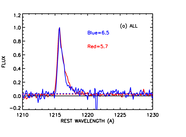
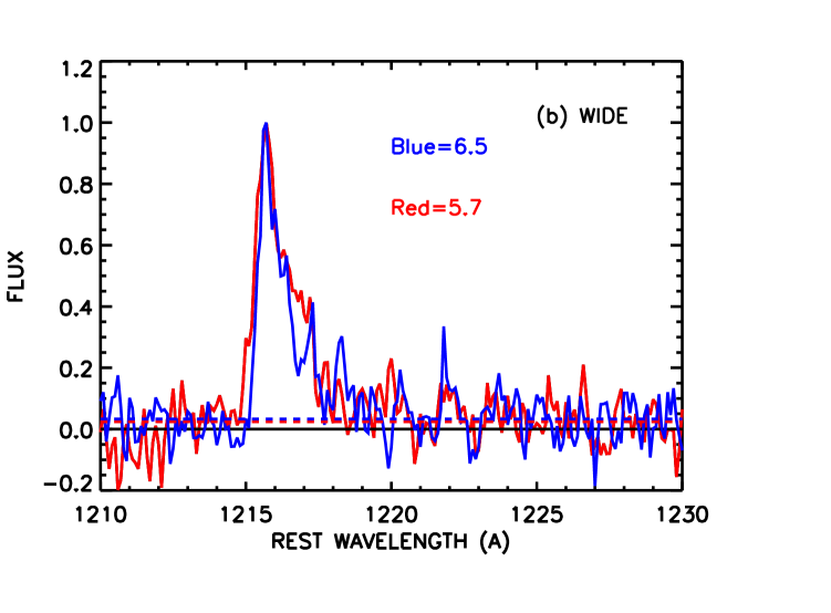
Figure 5.— (a) Comparison of the averaged spectra made from all the “quality one” spectra in the NB816 ($z=5.7$; red line) and NB912 ($z=6.5$; blue line) samples. These were formed by normalizing each individual spectrum’s Ly$\alpha$ peak to one and then averaging the normalized spectra. In each case we show the level of the continuum measured redward of the Ly$\alpha$ line with the dashed line of the same color. (b) Comparison of the averaged spectra made from only the FWHM$>1.6$ Å objects in the two samples. These wider spectra have a more developed red elbow.

The Ly$\alpha$ lines are poorly fit by a Gaussian because of the fairly sharp cut-off at the short-wavelength side. Thus, in order to provide a simple fit to the spectra, we used a demi-Gaussian consisting only of the long-wavelength side of the Gaussian together with a constant long-wavelength continuum, as shown in Figure 6 (green curve). This parameterization was introduced in H04. For each spectrum we convolved the demi-Gaussian with the instrument profile (blue dotted curve) and fitted the result to the observations using the IDL MPFIT programs of Markwardt (2009). We show this for (a) the full averaged spectrum at $z=5.7$; (b) the full averaged spectrum at $z=6.5$; (c) the wide averaged spectrum at $z=5.7$; (d) the wide averaged spectrum at $z=6.5$. We find that this simple model has sufficient freedom with its four free parameters (the normalization, the cut-off wavelength, the line width, and the red continuum level) to provide a good fit to all the spectra. (This is in agreement with H04’s conclusion for their $z=5.7$ line profile but not with Kashikawa et al. 2006, who found that they could not reproduce the red side of their $z=6.5$ line profile with this type of model.) In particular, the shape of the wider spectra are simply reproduced by an increase in the width of the Gaussian, and the short-wavelength drop in the observed lines is fully consistent with the abrupt cut-off in the model. We define the rest-frame FWHM of the lines as the half-width half-maximum (HWHM) of the Gaussian prior to truncation. We give the HWHM in the tables in the Appendix, together with the $1\sigma$ errors, for all the individual spectra.

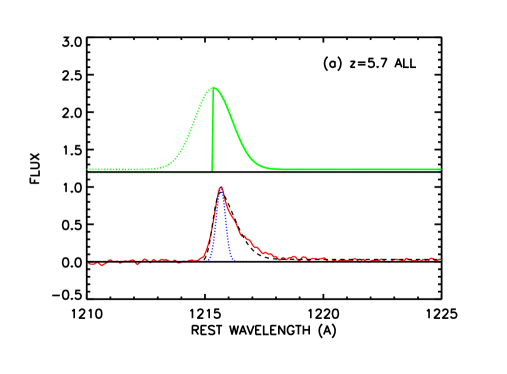
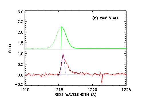
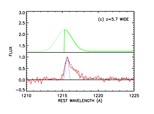
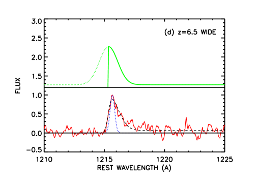
Figure 6.— Adopted fitting procedure. For each spectrum we fitted a demi-Gaussian consisting of the long-wavelength side of a Gaussian profile convolved through the instrument response. The free parameters are the normalization, the wavelength position, the width of the Gaussian, and the normalization of the long-wavelength continuum. We used the MPFIT programs of Markwardt (2009) to make the fit. We show the fits to the averaged spectra: (a) all $z=5.7$, (b) all $z=6.5$, (c) wide $z=5.7$, and (d) wide $z=6.5$. In each panel we show in the upper part the input-truncated Gaussian (green curve) and in the lower part the fit (black dashed curve) to the observed spectrum (red curve). The blue dotted line in the lower part shows the instrument response. We use the HWHM of the Gaussian (i.e., the FWHM of the demi-Gaussian) to characterize the width of the lines. The widths for the averaged spectra are (a) 0.94 Å, (b) 0.82 Å, (c) 1.26 Å, and (d) 0.90 Å.

For the average of all the spectra, the FWHM (as defined in the previous paragraph) is $0.98\pm 0.04$ Å at $z=5.7$ and $0.81\pm 0.08$ Å at $z=6.5$. The corresponding rest-frame equivalent widths, which we define as the area of the line divided by the red continuum level, are $34\pm 2$ Å at $z=5.7$ and $24\pm 3$ Å at $z=6.5$. This suggests that the equivalent widths have dropped slightly between the two redshifts. However, the error is primarily in the determination of the red continuum, and the difficulty of accurately measuring this quantity and the possibility of systematic errors should be kept in mind in assessing this result.

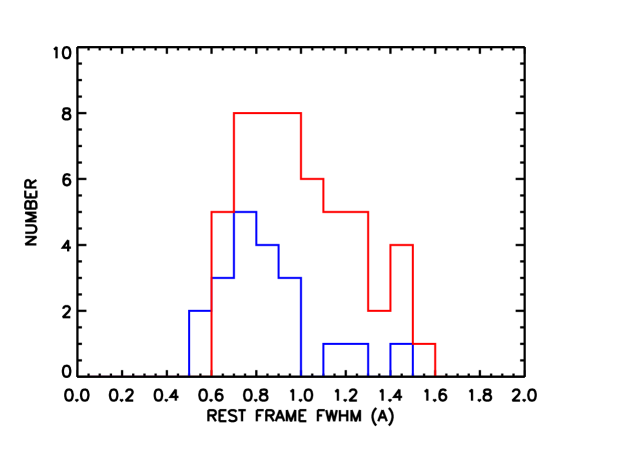
Figure 7.— Distribution of FWHM line widths obtained from the fitting procedure for the $z=5.7$ sample (red histogram) and for the $z=6.5$ sample (blue histogram).

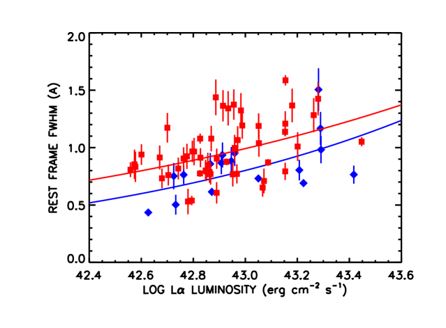
Figure 8.— Distribution of FWHM line widths obtained from the fitting procedure for the $z=5.7$ sample (red squares) and for the $z=6.5$ sample (blue diamonds). In both cases we show the $\pm 1\sigma$ errors. The blue and red lines show power-law fits of the form FWHM $=A~{}L_{\alpha}^{a}$.

The line widths are robustly measured and can be obtained for each of the individual spectra. However, the long-wavelength continuua are often too weak to be measured in the individual spectra, so we do not attempt to measure equivalent widths in the individual spectra. We compare the distribution of line widths in the two samples in Figure 7, where the red histogram shows the $z=5.7$ sample and the blue histogram shows the $z=6.5$ sample. There is just over a factor of two spread in the widths, which suggests that the spread in galaxy properties combines with the transfer effects to produce a fairly uniform output line with a velocity width in the range $150-360$ km s^-1. As with the averaged spectra, the lines are narrower at the higher redshift with a median value of $0.77$ Å at $z=6.5$ and $0.92$ Å at $z=5.7$. However, the difference is only marginally significant. A Mann-Whitney rank sum test rejects the two samples as being drawn from the same population at the $5\%$ confidence level.

Part of the spread in the line widths appears to be caused by a dependence of the FWHM on the Ly$\alpha$ luminosity, $L_{\alpha}$. In Figure 8 we show the dependence of the deconvolved FWHM measured with the fitting procedure on $L_{\alpha}$. Both the $z=5.7$ and the $z=6.5$ samples appear to show an increase of the width with luminosity. This is in contrast to Kashikawa et al. 2006, who suggested a slight increase with decreasing luminosity in their $z=6.5$ sample; see their Figure 11. The difference may arise from the higher resolution of the present observations and the wider range in $L_{\alpha}$. Ouchi et al. (2010), using Keck DEIMOS spectra, reverse the Kashikawa et al. 2006 result and find evidence at the 2.5 sigma level for a rise in the FWHM with luminosity. The effect is highly significant in our $z=5.7$ sample: a Mann-Whitney rank sum test shows that there is only a 0.005 probability that the population with $\log L_{\alpha}<42.9$ is drawn from the same distribution of FWHM as those at brighter luminosities. The Spearman correlation coefficient is 0.42 at a $3\sigma$ significance for the $z=5.7$ sample and 0.58 at a $2.3\sigma$ significance for the $z=6.5$ sample.

In each case we have fitted a power law of the form FWHM $=A~{}L_{\alpha}^{a}$ to the data. For $z=5.7$ we find $a=0.24\pm 0.07$, and for $z=6.5$ we find $a=0.31\pm 0.11$. These fits are shown by the red line ($z=5.7$) and the blue line ($z=6.5$) in Figure 8. There are many effects which could contribute to there being a relation between the observed line luminosity and the line width. Possibly the simplest interpretation is that the higher luminosity galaxies are more massive and the emerging L$\alpha$ line is wider. However, detailed modeling, including all of the line transfer effects, is necessary to fully interpret this result.

3.2. Number Counts

The average number of objects detected per SuprimeCam field is 12.4 at $z=5.7$ and 3.9 at $z=6.5$. The observed ranges of $6-18$ per field at $z=5.7$ and $1-7$ per field at $z=6.5$ are fully consistent with the spread expected from the small number statistics. We do not require any additional effects from cosmic variance to understand this, though such effects may be expected to be present.

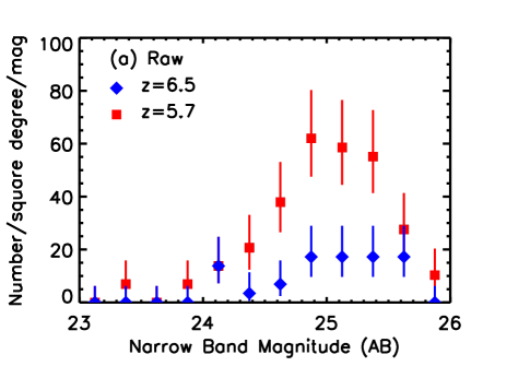
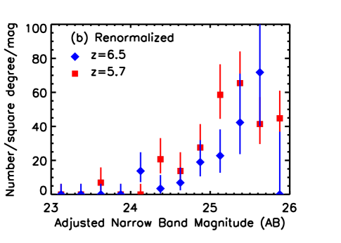
Figure 9.— (a) Observed number counts vs. narrowband magnitude [red squares—NB816 ($z=5.7$) selected galaxies; blue diamonds—NB912 ($z=6.5$) selected galaxies]. In both cases the error bars are $\pm 1\sigma$ based on the number of objects in each bin. (b) Comparison of the counts in the NB816 sample (the magnitudes were adjusted to equivalent NB912 magnitudes by correcting for the relative luminosity distance), corrected for incompleteness in the photometric catalog, with the counts in the NB912 sample, also corrected for incompleteness. Between 23 and 25.25, where both sets of counts are near complete, the NB816 number counts need to be multiplied by a factor of $0.47\pm 0.13$ to match the NB912 counts.

The similarities of the depths of the fields and of the shapes and rest-frame widths of the two filters allow us to make a simple estimate of the decrease in the number of Ly$\alpha$ emitters with increasing redshift directly from the number counts. The number counts in the two redshift ranges are shown versus narrowband magnitude in Figure 9(a). We denote the $z=5.7$ counts by red squares and the $z=6.5$ counts by blue diamonds. As would be expected from the initial selection, the counts rise smoothly to near $N_{\rm AB}=25.0-25.5$ and then drop rapidly at fainter magnitudes. In this discussion and in the derivation of the LF in the next subsection, we shall restrict to a sample with $N_{\rm AB}<25.25$ where we believe the samples in both bands are substantially complete both in the initial selection and in the spectroscopic followup.

To compare the number counts, we corrected the NB816 magnitudes to equivalent NB912 magnitudes by adding the difference in magnitude corresponding to the relative luminosity distance. In Figure 9(b) we compare the $z=5.7$ counts (for the equivalent NB912 magnitudes), corrected for the initial photometric catalog incompleteness, with the $z=6.5$ counts, corrected in the same way. (The photometric catalog incompleteness at these magnitudes is small; see Figure 3.) The ratio of the numbers of galaxies above the (equivalent) NB912 magnitude of 25.25 at $z=6.5$ and at $z=5.7$ is $0.47\pm 0.13$. The error is $\pm 1\sigma$. The shapes are fully consistent, and a single multiplicative renormalization alone is sufficient to match the two sets of counts.

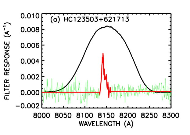
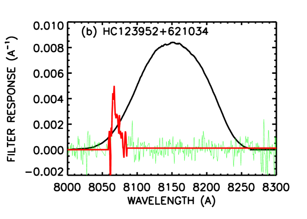
Figure 10.— Illustration of the flux computation for two of the $z=5.7$ Ly$\alpha$ emitters. The curves show the NB816 filter response (black); the adopted spectrum in the observed frame (red), which corresponds to a constant value of 0.025 of the peak in the spectrum for the red continuum, zero for the blue continuum, and the actual spectrum between the rest-frame wavelengths of 1214.5 to 1218.5 Å; and the actual spectrum outside this range (green). (a) A Ly$\alpha$ emitter that is well centered on the filter. Nearly 90% of the contribution to the narrowband magnitude comes from the emission line. (b) A Ly$\alpha$ emitter lying at the short-wavelength end of the filter. Almost 60% of the contribution to the narrowband magnitude comes from the continuum.

3.3. Luminosity Functions

In order to compute the Ly$\alpha$ luminosities of the individual galaxies and the cosmological volumes sampled by the survey, we must allow for the shapes of the narrowband selection filters. This is made more complex by the presence of the continuum, which slightly pulls the selection to the short-wavelength side of the filter, as can be seen in Figure 2 and also in Figure 13 of H04 and in Figure 3 of Kashikawa et al. (2006). The continuum is extremely faint and often undetected in the spectra and even in the continuum images, so this effect is not easy to model exactly, but it is necessary to include it to make a correct conversion from the narrowband magnitude to a line flux.

To convert the narrowband magnitude to a line flux, we convolve the observed spectrum through the narrowband filter. However, outside the line itself, defined as the portion of the spectrum between rest-frame wavelengths 1214.5 and 1218.5 Å, we use a model continuum. At redder wavelengths we use a continuum with a flux of 0.025 times the peak in the line seen in the individual spectra (see Figure 5). The adopted ratio is based on that measured in the averaged spectrum. At bluer wavelengths we assume that the continuum is zero. We use the narrowband magnitude to flux calibrate the spectrum and hence to determine the line flux.

We illustrate the procedure in Figure 10, where we show the NB816 filter response (black curve), the adopted spectrum (red curve), and the actual spectrum (green curve) in the wavelength range where we use the model continuum instead. In Figure 10(a) we show an emitter that is well centered on the filter. For this object nearly 90% of the contribution to the narrowband magnitude comes from the emission line, and the conversion to an emission-line flux should be robust. In Figure 10(b) we show an emitter lying at the short-wavelength end of the filter. For this object almost 60% of the contribution to the narrowband magnitude comes from the continuum. In order to avoid the uncertainty associated with the flux conversion in objects like this, we restrict our subsequent analysis to galaxies with Ly$\alpha$ wavelengths where the filter transmission is above 25% of the peak value. This eliminates objects where the narrowband flux is continuum dominated. In column 11 of Tables 5, 6, and 7 in the Appendix we list the derived Ly$\alpha$ luminosities for each object.

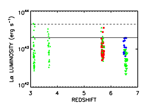
Figure 11.— The observed Ly$\alpha$ luminosity in each of the redshift intervals (red squares—$z=5.7$ Ly$\alpha$ emitters; blue diamonds—$z=6.5$ Ly$\alpha$ emitters). Only objects with narrowband magnitudes less than 25.25 at a wavelength that has a filter response above 0.25 are shown. In order to avoid lensing effects, objects within a $10^{\prime}$ radius of the center of A370 are excluded. For comparison, spectroscopically identified objects in Ouchi et al. (2008) (green solid triangles) and in both Taniguchi et al. (2005) and Kashikawa et al. (2006) (green open downward pointing triangles) are also shown. The dashed (solid) horizontal line shows the maximum luminosity object of $\sim 4.5\times 10^{43}$ erg s^-1 ($\sim 2.0\times 10^{43}$ erg s^-1) observed at $z\sim 3$ ($z\sim 6.5$).

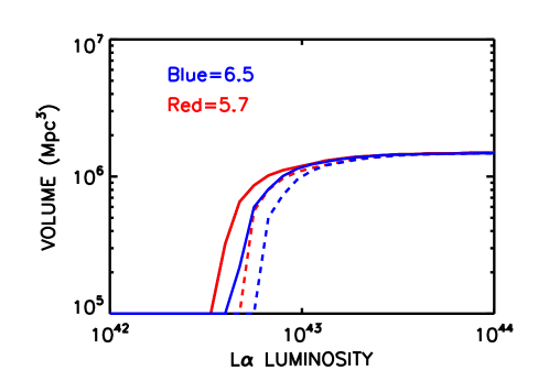
Figure 12.— The observable comoving volume as a function of Ly$\alpha$ luminosity (blue curves—$z=6.5$; red curves—$z=5.7$). The solid (dashed) curves are for a limiting narrowband magnitude of 25.5 (25.25). We restrict to wavelengths where the filter transmission is above 25% of the peak value.

We show the distribution of Ly$\alpha$ luminosities for the samples at $z=5.7$ (red squares) and $z=6.5$ (blue diamonds) in Figure 11. We only show objects with $N_{\rm AB}<25.25$ that have a filter transmission above 25% of the peak. We compare with spectroscopic samples at $z=3.1,3.7$, and $5.7$ from Ouchi et al. (2004) (green solid triangles) and at $z=6.5$ from both Taniguchi et al. (2005) and Kashikawa et al. (2006) (green open downward pointing triangles). At $z=5.7$ our distribution of luminosities is very similar to that of Ouchi et al. (2008), despite some methodological differences. (For example, Ouchi et al. do not account for the filter shape in computing the luminosities but instead deal with this in subsequent simulations.) However, the $z=6.5$ samples of Kashikawa et al. and Taniguchi et al. are systematically lower than those in the present work. It appears from their description that their luminosities are based on uncorrected $2^{\prime\prime}$ diameter aperture magnitudes. (The Ouchi et al. 2008 luminosities are based on corrected $2^{\prime\prime}$ diameter aperture magnitudes.) The correction to total magnitudes would then raise their luminosities by factors of $1.3-1.4$, which could account for a substantial part of the difference. They also assume a rectangular shape for the narrowband filter in computing the luminosities (Taniguchi et al. 2005’s Equations 6 and 7), which could also result in differences.

The peak luminosities seen in our present samples at $z=5.7$ and $z=6.5$ are slightly more than a factor of two less than those seen near $z=3$. This can be fully understood in terms of the intergalactic absorption correction, and it appears that the intrinsic luminosities of the brightest emitters are hardly changing from $z=6.5$ to $z=3.1$. However, this simple analysis is dependent on the number of objects in each redshift sample, and the evolution is best treated by looking at the LFs, which we now do.

In order to compute the LFs, we must determine the accessible comoving volume as a function of luminosity. Here again the shape of the filter transmission makes the calculation more complicated. For a rectangular filter the volume is fixed above the detection threshold. However, for more complex filter shapes, the wavelength range is a function of the luminosity and the selection magnitude. For a given limiting magnitude, more luminous objects will be seen over a wider range of redshifts, since they can still be detected at lower filter transmissions.

In order to compute the observable comoving volume as a function of luminosity and limiting narrowband magnitude, we used the averaged spectral profiles of the emitters at $z=5.7$ and $z=6.5$ (Figure 5). We normalized the appropriate spectrum for the filter (i.e., the $z=5.7$ spectrum for the NB816 filter and the $z=6.5$ spectrum for the NB912 filter) to correspond to a given line luminosity and then stepped this through the filter, calculating the narrowband magnitude at each redshift. This allowed us to determine the redshift range over which a line of this luminosity would produce a narrowband magnitude above the narrowband magnitude limit. We show the observed volumes at $z=6.5$ (blue curves) and at $z=5.7$ (red curves) as a function of the Ly$\alpha$ luminosity in Figure 12. The solid lines show the values for a limiting narrowband magnitude of 25.5, and the dashed lines for 25.25. For 25.25, which we use in the subsequent calculations, the volume drops rapidly below $\sim 5.6\times 10^{42}$ erg s^-1 at $z=5.7$ and below $\sim 6.7\times 10^{42}$ erg s^-1 at $z=6.5$.

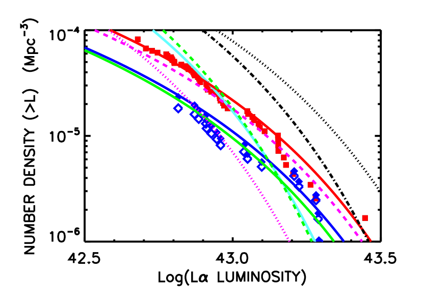
Figure 13.— The cumulative Ly$\alpha$ LFs at $z=5.7$ (red squares) and $z=6.5$ (blue diamonds). The red and blue solid curves show the maximum likelihood fits to a Schechter function with an $\alpha=-1.5$ slope. The black dash-dotted curve shows the $z=5.7$ cumulative LF from Ouchi et al. (2008) and the black dotted curve shows the $z=5.7$ cumulative LF of Shimasaku et al. (2006), both based on their photometric samples. The purple dashed (dotted) curve shows the $z=5.7$ ($z=6.5$) cumulative LF from the spectroscopic sample of Malhotra & Rhoads (2004). The green solid (dashed) curve shows the $z=6.5$ cumulative luminosity function from the spectroscopic (photometric) sample of Kashikawa et al. (2006) while the solid cyan curve shows that of Ouchi et al. (2010) which is also primarily photometric.

We first computed the cumulative LF, which is simply the sum of the inverse observable volumes above a given Ly$\alpha$ luminosity. In order to avoid lensing effects, we excluded the central $10^{\prime}$ region in the A370 field and corrected the volume accordingly. Only objects with narrowband magnitudes brighter than 25.25 and lying above 25% of the maximum response in the filter are included in the sample, and the observable volumes were computed to correspond to this selection. We show the results in Figure 13. For the $z=6.5$ sample we show both the cumulative LF prior to any incompleteness correction (blue open diamonds) and that with the spectroscopic and photometric incompleteness correction included (blue solid diamonds). The correction is small with this magnitude selection. For the $z=5.7$ sample, where the correction is even smaller, we show only the incompleteness corrected LF (red solid squares).

The red and blue solid curves show the maximum likelihood fits to the two data samples for a Schechter function with slope $\alpha=-1.5$. Because of the limited dynamic range of the data, we have not attempted to fit for the slope of the Schechter function but rather computed $L_{\star}$ for fixed values of this quantity. The normalization $\phi_{\star}$ is calculated to match the observed number of sources over the observed luminosity range. For $\alpha=-1.5$ and $z=5.7$, the fitted parameters are $\log L_{\star}=43.0^{43.3}_{42.8}$ and $\phi_{\star}=1.1\pm 0.2\times 10^{-4}$ Mpc^-3. For $\alpha=-1.5$ and $z=6.5$, they are $\log L_{\star}=43.0^{43.6}_{42.7}$ and $\phi_{\star}=0.6\pm 0.2\times 10^{-4}$ Mpc^-3. Here the luminosities are in units of erg s^-1, and the range is the 68% confidence limit. Over the fitted range the $z=6.5$ counts are $0.56\pm 0.17$ of the $z=5.7$ counts for the $\alpha=-1.5$ case and the characteristic luminosity is unchanged consistent with our previous discussion of the number counts. We summarize the fitted parameter for varying values of $\alpha$ in table 4.

Table 4Luminosity function fits

Redshift	$\alpha$	Log $\L_{\star}$	$\phi_{\star}$
		erg s-1	$10^{-4}$ Mpc-3
5.7	-1.0	$42.9^{43.1}_{42.7}$	$1.7\pm 0.3$
5.7	-1.5	$43.0^{43.3}_{42.8}$	$1.1\pm 0.2$
5.7	-2.0	$43.2^{43.7}_{42.9}$	$0.5\pm 0.1$
6.5	-1.0	$42.9^{43.3}_{42.6}$	$0.7\pm 0.2$
6.5	-1.5	$43.0^{43.6}_{42.7}$	$0.6\pm 0.2$
6.5	-2.0	$43.1^{44.3}_{42.7}$	$0.3\pm 0.1$

In Figure 13 we also compare the present data with measurements from the literature. In all cases we show the maximum likelihood fits for a Schechter function with slope $\alpha=-1.5$. Our $z=5.7$ LF agrees quite well with the Malhotra & Rhoads (2004) LF based on their spectroscopic sample (purple dashed curve), but it is about a factor of slightly more than two lower than either the Ouchi et al. (2008) (black dash-dotted curve) or the Shimasaku et al. (2006) (black dotted curve) LFs, which are based on their photometric samples. Our $z=6.5$ LF is only slightly above the Kashikawa et al. (2006) LF based on their spectroscopic sample (green solid curve). It is similar to the Malhotra & Rhoads (2004) spectroscopically based sample (purple dotted curve) at low luminosities, though the present sample clearly has more objects at high luminosities than this fit would predict. It is about a factor of two lower than the Kashikawa et al. (2006) photometrically based sample (green dashed curve) or the very similar Ouchi et al. (2010) LF (cyan curve) at low luminosities, but it is higher at the bright end.

The largest differences appear to be with the photometrically based LFs of Ouchi et al. (2008) and Kashikawa et al. (2006) and Ouchi et al. (2010). The presently derived LFs are typically about a factor of two lower. This is not a consequence of the magnitude calibrations, since, as we have discussed previously, both the Ouchi et al. and the Kashikawa et al. magnitude measurements are fainter than the present photometry, and this would have the opposite effect (i.e., it would raise our LFs relative to theirs rather than reduce them).

The real reason for the reduction in our LFs relative to theirs seems to come from our having excluded the spectroscopically unconfirmed objects. Ouchi et al. (2008) observed 29 of their photometrically selected galaxies and identified 17 as Ly$\alpha$ emitters. However, they estimated the contamination based on only the objects brighter than a narrowband magnitude of 24.5, where three-quarters of the objects were identified, and concluded that the maximum contamination was 25%. Since this was small, they did not apply a correction. However, the numbers on which this calculation are based are small, and the probability of incorrect selections may be expected to increase as we move to fainter magnitudes. Thus, the bright selection is likely to be inappropriate for the full sample.

In the present work we could not spectroscopically confirm approximately half of our photometrically selected objects in our 25.5 magnitude limited sample. Thus, the factor of two difference between our $z=5.7$ LF and the Ouchi et al. (2008) $z=5.7$ LF may be entirely due to this. It is possible that some of the photometrically selected objects that are unconfirmed in the spectroscopy are genuine Ly$\alpha$ emitters where the spectroscopy was problematic. However, for many, even with multiple observations we were unable to confirm spectroscopically the objects as emitters. We therefore think the present spectroscopically based Ly$\alpha$ LFs represent the best estimate, and the photometric LFs may be viewed as extreme upper limits.

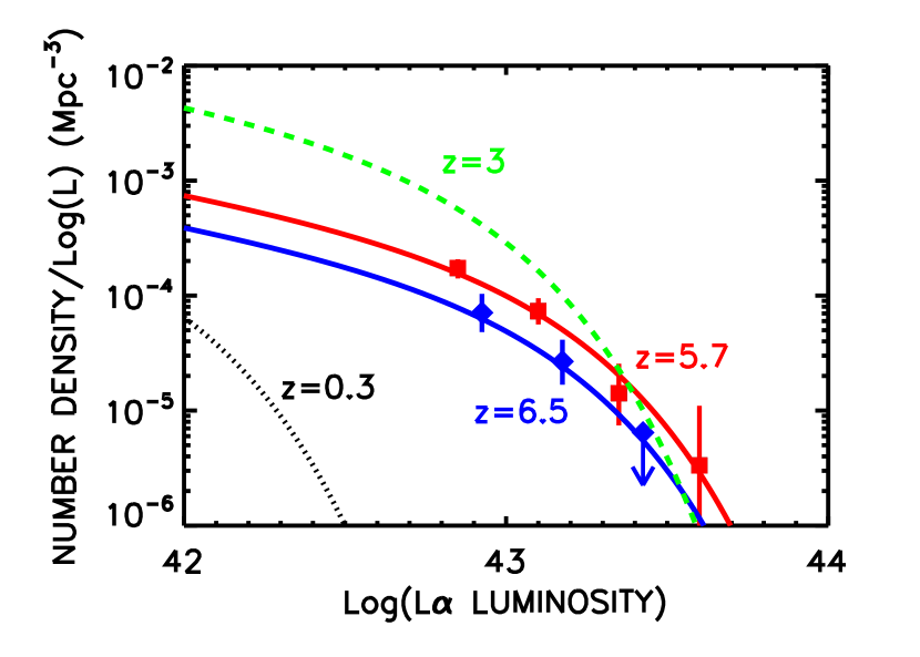
Figure 14.— The Ly$\alpha$ LF at $z=5.7$ is shown with red squares and that at $z=6.5$ is shown with blue diamonds. The errors are $\pm 1\sigma$ based on the number of objects in each luminosity bin. The red and blue solid curves show maximum likelihood fits to a Schechter function with an $\alpha=-1.5$ slope. The green dashed curve shows the $z=3.1$ LF measured by Ouchi et al. (2008) using their maximum likelihood fit for $\alpha=-1.5$. The black dotted curve shows the local Ly$\alpha$ LF at $z=0.3$ derived by Cowie et al. (2010) from GALEX spectroscopy.

In Figure 14 we show the differential LFs at $z=6.5$ (blue diamonds) and at $z=5.7$ (red squares). The error bars are $\pm 1\sigma$ based on the Poisson errors corresponding to the number of objects in the bin. For the $z=6.5$ case we also show the $1\sigma$ upper limit at the highest luminosity with the downward pointing arrow. We show the maximum likelihood fits for $\alpha=-1.5$ with the blue and red curves. In the figure we compare the present LFs with those measured at lower redshifts. We show the LF at $z=0.3$ derived by Cowie et al. (2010) using GALEX spectroscopy with the black dotted curve. We show the LF at $z=3.1$ from Ouchi et al. (2008) with the green dashed curve. Other determinations at this redshift by van Breukelen et al. (2005), Gronwall et al. (2007), and Cowie & Hu (1998) are extremely similar, and we do not plot them separately.

Clearly the low-redshift evolution of the Ly$\alpha$ LF between $z=0.3$ and $z=3$ is much more spectacular than that seen at the higher redshifts. Locally there are very few luminous Ly$\alpha$ objects and very little light density in the Ly$\alpha$ emission line. However, at $z>3$ the maximum luminosity is relatively invariant, and the number density is falling off slowly with increasing redshift. For a fixed $\alpha=-1.5$ the light density in the Ly$\alpha$ line at $z=5.7$ is about 22% of that at $z=3.1$, and the light density in the Ly$\alpha$ line at $z=6.5$ is about 11% of that at $z=3.1$. When the values are corrected for the effects of the intergalactic scattering, which substantially reduce the observed Ly$\alpha$ luminosities relative to the intrinsic luminosities, the change between $z=3.1$ and $z=5.7$ will be less, probably no more than a decrease of a factor of 2. We shall make a more detailed comparison to the evolution of the UV continuum light at these redshifts in a subsequent paper (L. Cowie et al. 2010, in preparation).

Table 5$z=5.7$ Ly$\alpha$ Emitters

Number	Name	R.A.	Decl.	$N$	$I$	Redshift	Expo	Qual	FWHM	Log(L)
		(J2000)	(J2000)	(AB)	(AB)		(hrs)		Å	erg/s
(1)	(2)	(3)	(4)	(5)	(6)	(7)	(8)	(9)	(10)	(11)
1	HC123818+621621	189.57700	62.27261	$23.26$	$25.28$	5.7275	1	2	$1.31\pm 0.04$	43.55
2	HC124128+622022	190.36998	62.33969	$23.32$	$26.25$	5.6947	4	1	$1.05\pm 0.03$	43.44
3	HC123744+621145	189.43600	62.19588	$23.95$	$25.88$	5.6680	3	1	$1.28\pm 0.14$	43.26
4	HC221832-002844	334.63602	0.4790830	$23.96$	$25.48$	5.6800	5	1	$0.82\pm 0.02$	43.20
5	HC124115+622258	190.31601	62.38280	$24.03$	$25.60$	5.7020	2	1	$1.36\pm 0.14$	43.18
6	HC221811-000500	334.54807	0.08355599	$24.06$	$26.16$	5.7086	3	1	$0.79\pm 0.07$	43.15
7	HC124125+622050	190.35699	62.34750	$24.12$	$26.43$	5.7137	2	1	$1.42\pm 0.13$	43.17
8	HC221654-000538	334.22900	0.09402800	$24.12$	$26.28$	5.6758	3	1	$1.20\pm 0.10$	43.15
9	HC221720-002007	334.33701	0.3353610	$24.30$	$25.84$	5.6706	3	1	$0.65\pm 0.07$	43.06
10	HC221720-001737	334.33701	0.2938329	$24.30$	$25.84$	5.6672	2	1	$1.58\pm 0.04$	43.15
11	HC123503+621713	188.76300	62.28719	$24.31$	$27.67$	5.6975	1	1	$1.17\pm 0.12$	43.04
12	HC221802-001431	334.50903	0.2421390	$24.31$	$26.19$	5.6738	4	1	$0.87\pm 0.02$	43.08
13	HC221843-004439	334.67996	0.7441939	$24.44$	$26.22$	5.6550	2	1	$0.83\pm 0.09$	43.10
14	HC221728-001918	334.37000	0.3217220	$24.49$	$25.49$	5.6426	4	1	$1.42\pm 0.14$	43.27
15	HC221733-002216	334.38800	0.3713330	$24.56$	$26.15$	5.6531	3	1	$0.77\pm 0.08$	43.09
16	HC123651+621936	189.21498	62.32680	$24.58$	$26.33$	5.6750	3	1	$0.77\pm 0.08$	42.96
17	HC123652+622152	189.21700	62.36460	$24.60$	$27.18$	5.6861	6	1	$0.87\pm 0.02$	42.92
18	HC221705-001300	334.27301	0.2169169	$24.61$	$26.33$	5.6700	3	1	$1.06\pm 0.12$	42.97
19	HC124033+621838	190.14000	62.31069	$24.61$	$26.48$	5.6502	1	1	$1.13\pm 0.03$	43.15
20	HC123626+620346	189.11000	62.06300	$24.65$	$27.35$	5.6998	2	1	$1.04\pm 0.04$	42.91
21	HC024015-012946	40.065208	-1.496333	$24.70$	$27.36$	5.7105	1	1	$0.95\pm 0.10$	42.90
22	HC123613+620748	189.05600	62.13000	$24.70$	$26.12$	5.6345	1	1	$0.76\pm 0.10$	42.95
23	HC023953-013627	39.972916	-1.607750	$24.70$	$25.79$	5.6928	2	1	$0.84\pm 0.10$	42.85
24	HC221656-001446	334.23499	0.2463060	$24.71$	$26.53$	5.6621	2	1	$1.32\pm 0.15$	42.98
25	HC123903+621444	189.76300	62.24569	$24.71$	$26.58$	5.7374	1	1	$0.70\pm 0.10$	43.07
26	HC170647+434520	256.69598	43.75569	$24.78$	$26.67$	5.7084	6	1	$1.43\pm 0.15$	42.88
27	HC170648+435813	256.70099	43.97050	$24.78$	$26.81$	5.7265	2	1	$1.37\pm 0.13$	42.95
28	HC221731-000937	334.38202	0.1602780	$24.79$	$26.74$	5.6843	5	1	$0.78\pm 0.09$	42.86
29	HC024035-013626	40.146709	-1.607500	$24.79$	$27.24$	5.6796	4	2	$1.50\pm 0.18$	42.87
30	HC123835+620643	189.64702	62.11200	$24.83$	$26.87$	5.6938	1	2	$0.84\pm 0.12$	42.80
31	HC221739-002545	334.41299	0.4292219	$24.84$	$25.90$	5.6599	2	1	$0.99\pm 0.11$	42.95
32	HC221710-001240	334.29199	0.2112780	$24.85$	$25.88$	5.6221	2	1	$1.42\pm 0.07$	43.27
33	HC124043+621534	190.18199	62.25969	$24.86$	$27.85$	5.7033	3	1	$1.24\pm 0.13$	42.84
34	HC221707-002744	334.28000	0.4624719	$24.86$	$26.81$	5.7241	1	1	$1.36\pm 0.13$	42.91
35	HC024059-012737	40.246414	-1.460472	$24.87$	$26.18$	5.7224	5	1	$0.90\pm 0.08$	42.89
36	HC221716-001325	334.31799	0.2238609	$24.89$	$26.09$	5.6444	3	1	$1.03\pm 0.11$	43.05
37	HC123717+621759	189.32401	62.29988	$24.90$	$26.55$	5.6610	2	3	$1.88\pm 0.16$	42.91
38	HC024138-013616	40.411419	-1.604611	$24.92$	$26.34$	5.6841	3	1	$0.96\pm 0.11$	42.80
39	HC024104-012750	40.267582	-1.464000	$24.93$	$26.50$	5.7237	5	1	$1.22\pm 0.12$	42.88
40	HC170704+435135	256.76898	43.85988	$24.93$	$25.86$	5.6157	3	2	$0.74\pm 0.16$	42.98
41	HC221706-001222	334.27798	0.2063060	$24.95$	$26.58$	5.6510	2	1	$0.60\pm 0.09$	42.88
42	HC170704+435811	256.76801	43.96980	$24.97$	$26.08$	5.6992	1	1	$0.73\pm 0.09$	42.74
43	HC024056-012845	40.235203	-1.479333	$24.97$	$27.56$	5.7063	6	1	$0.96\pm 0.09$	42.79
44	HC024121-013220	40.340084	-1.539055	$25.00$	$26.70$	5.6759	5	1	$0.53\pm 0.04$	42.79

Table 5$z=5.7$ Ly$\alpha$ Emitters

Number	Name	R.A.	Decl.	$N$	$I$	Redshift	Expo	Qual	FWHM	Log(L)
		(J2000)	(J2000)	(AB)	(AB)		(hrs)		Å	erg/s
(1)	(2)	(3)	(4)	(5)	(6)	(7)	(8)	(9)	(10)	(11)
45	HC024038-013500	40.161293	-1.583389	$25.01$	$26.81$	5.7063	3	1	$0.92\pm 0.10$	42.77
46	HC221733-004202	334.39001	0.7005829	$25.01$	$26.81$	5.6180	2	1	$1.00\pm 0.12$	43.20
47	HC170657+434626	256.73898	43.77400	$25.02$	$25.80$	5.6599	5	1	$1.07\pm 0.11$	42.86
48	HC221816-003647	334.56903	0.6131939	$25.06$	$26.42$	5.7314	1	1	$0.76\pm 0.09$	42.86
49	HC124052+621119	190.21700	62.18880	$25.07$	$26.79$	5.6835	1	1	$0.62\pm 0.03$	42.72
50	HC123516+620508	188.81900	62.08561	$25.08$	$26.43$	5.7220	1	1	$0.53\pm 0.11$	42.77
51	HC124130+622621	190.37903	62.43938	$25.10$	$26.47$	5.6560	1	3	$0.73\pm 0.04$	42.91
52	HC221752-003615	334.47000	0.6043059	$25.12$	$28.08$	5.7330	1	1	$0.80\pm 0.09$	42.84
53	HC221740-002414	334.42004	0.4040830	$25.13$	$25.95$	5.6350	4	1	$1.18\pm 0.10$	43.05
54	HC024029-013919	40.120998	-1.655500	$25.15$	$26.15$	5.6427	2	1	$1.02\pm 0.12$	42.95
55	HC124107+622316	190.28101	62.38780	$25.15$	$27.03$	5.6858	2	1	$0.70\pm 0.09$	42.66
56	HC124103+622152	190.26601	62.36460	$25.16$	$26.50$	5.7430	2	1	$1.04\pm 0.10$	42.94
57	HC024042-013316	40.176788	-1.554556	$25.18$	$29.33$	5.6543	6	1	$0.79\pm 0.06$	42.85
58	HC221845-003405	334.69000	0.5683060	$25.18$	$27.62$	5.6909	4	1	$0.73\pm 0.08$	42.67
59	HC123607+620838	189.03300	62.14411	$25.20$	$27.10$	5.6400	2	1	$0.85\pm 0.10$	42.95
60	HC221652-001639	334.22000	0.2777499	$25.20$	$28.89$	5.6589	4	1	$1.07\pm 0.04$	42.82
61	HC170614+434815	256.56201	43.80438	$25.23$	$102.2$	5.6655	1	2	$0.90\pm 0.13$	42.70
62	HC123952+621034	189.97000	62.17630	$25.25$	$27.43$	5.6356	1	1	$1.19\pm 0.11$	42.98
63	HC170707+435530	256.78299	43.92511	$25.25$	$26.07$	5.6992	4	1	$0.91\pm 0.10$	42.67
64	HC024111-012855	40.299500	-1.482222	$25.25$	$26.40$	5.6954	4	1	$0.72\pm 0.03$	42.67
65	HC123609+620244	189.03897	62.04569	$25.26$	$30.28$	5.7183	1	1	$1.29\pm 0.14$	42.72
66	HC123612+620420	189.05000	62.07230	$25.32$	$27.52$	5.7410	1	1	$0.77\pm 0.02$	42.82
67	HC221810-003622	334.54199	0.6061940	$25.35$	$27.46$	5.6885	2	3	$0.94\pm 0.13$	42.57
68	HC123821+621046	189.59100	62.17961	$25.39$	$26.45$	5.6490	2	2	$1.17\pm 0.10$	42.83
69	HC170641+440756	256.67099	44.13230	$25.40$	$102.2$	5.6923	1	1	$0.93\pm 0.08$	42.60
70	HC221658-000836	334.24402	0.1433890	$25.41$	$26.88$	5.7353	2	1	$0.90\pm 0.09$	42.76
71	HC221725-000752	334.35501	0.1312779	$25.45$	$26.88$	5.7509	1	1	$0.98\pm 0.10$	42.93
72	HC221904-002520	334.76797	0.4224439	$25.46$	$101.9$	5.6242	2	1	$1.03\pm 0.12$	42.96
73	HC123532+621445	188.88399	62.24589	$25.46$	$29.18$	5.7026	1	3	$0.83\pm 0.13$	42.57
74	HC221658-001849	334.24500	0.3137220	$25.48$	$26.67$	5.6281	2	1	$1.34\pm 0.14$	42.93
75	HC221909-004121	334.79001	0.6893330	$25.49$	$27.54$	5.6882	2	2	$1.17\pm 0.13$	42.59
76	HC124015+621739	190.06601	62.29419	$25.49$	$29.16$	5.6913	2	1	$0.85\pm 0.12$	42.57
77	HC124154+622439	190.47501	62.41088	$25.49$	$102.2$	5.7448	2	1	$0.91\pm 0.08$	42.82
78	HC123558+621017	188.99498	62.17150	$25.51$	$29.42$	5.6718	2	3	$2.35\pm 0.20$	42.58
79	HC124007+621245	190.03101	62.21269	$25.51$	$27.29$	5.7388	1	1	$0.81\pm 0.09$	42.74
80	HC221750-002907	334.45898	0.4854440	$25.53$	$28.21$	5.6945	1	3	$0.20\pm 0.04$	42.50
81	HC024031-013230	40.132500	-1.541778	$25.57$	$-27.44$	5.7104	2	1	$1.15\pm 0.04$	42.57
82	HC221744-004024	334.43600	0.6734719	$25.58$	$28.61$	5.6860	2	2	$1.11\pm 0.03$	42.54
83	HC221757-004118	334.48898	0.6885830	$25.68$	$101.9$	5.6845	1	2	$0.85\pm 0.11$	42.47
84	HC221846-003156	334.69299	0.5324170	$25.68$	$26.67$	5.6409	1	1	$0.76\pm 0.09$	42.70
85	HC123756+622415	189.48500	62.40438	$25.74$	$28.84$	5.6499	1	1	$0.90\pm 0.12$	42.60
86	HC221812-004330	334.55197	0.7251110	$25.77$	$27.86$	5.6440	1	1	$1.17\pm 0.12$	42.70
87	HC221840-003720	334.67004	0.6223610	$25.79$	$27.76$	5.6590	2	2	$0.57\pm 0.02$	42.55
88	HC221802-003007	334.51001	0.5020279	$25.80$	$27.02$	5.6598	2	3	$1.18\pm 0.05$	42.53

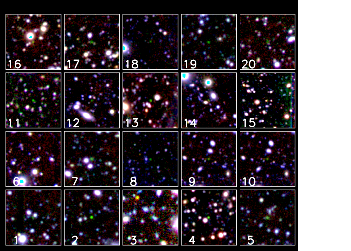
Figure A1.— Images of the spectroscopically confirmed $z=5.7$ Ly$\alpha$ emitter sample. For each object we show a $40^{\prime\prime}$ thumbnail around the emitter with blue=$R$-band, green=F816 narrowband, and red=$z$-band. The emitter appears as a green object at the center of the thumbnail. The numerical label corresponds to the number in Table A2 and Figure A2.

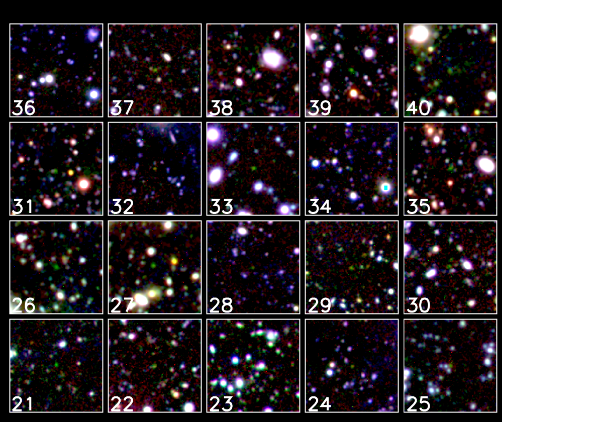
Figure A1.— Images of the spectroscopically confirmed $z=5.7$ Ly$\alpha$ emitter sample (continued).

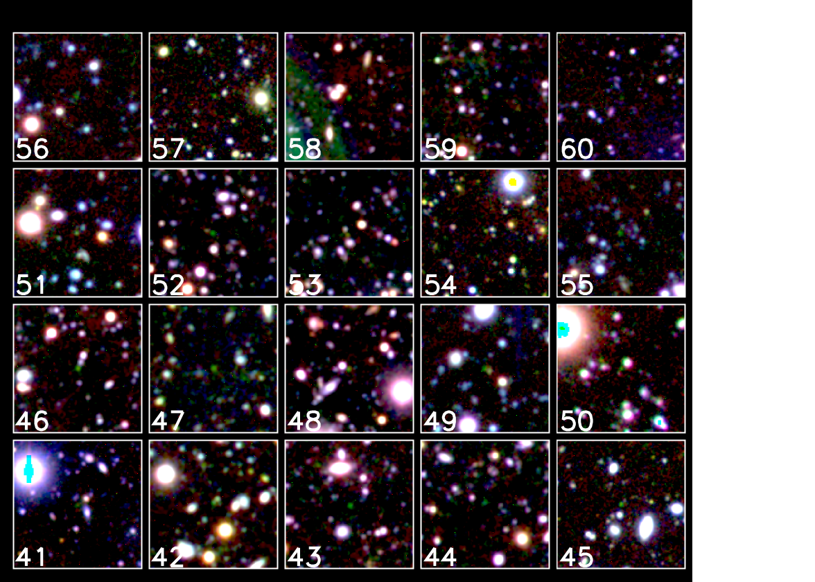
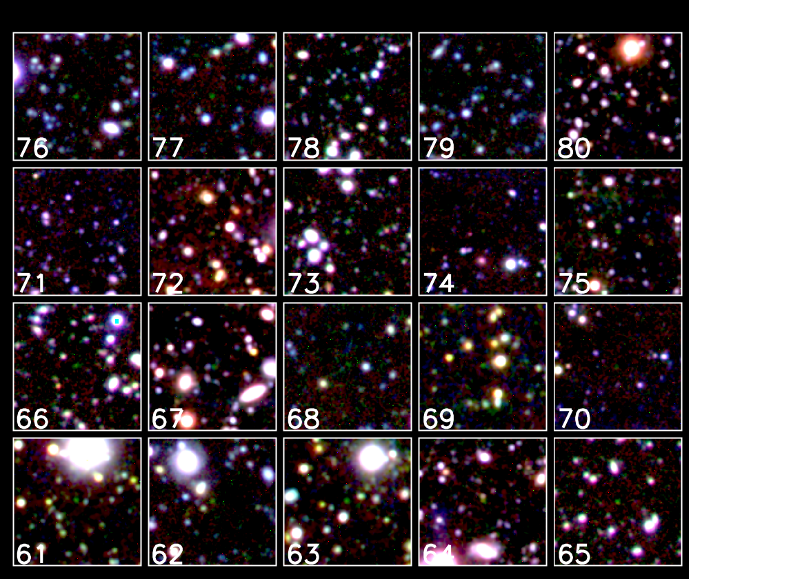
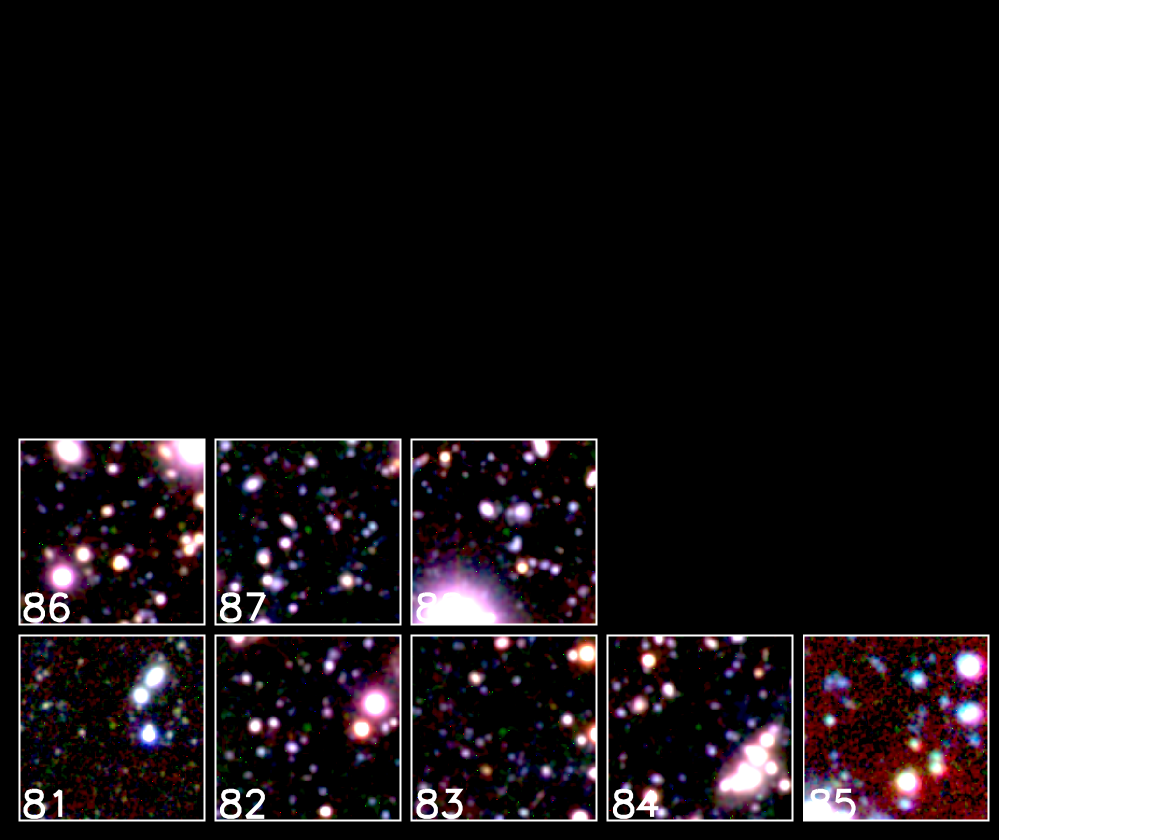
Figure A1.— Images of the spectroscopically confirmed $z=5.7$ Ly$\alpha$ emitter sample (continued).

Figure A1.— Images of the spectroscopically confirmed $z=5.7$ Ly$\alpha$ emitter sample (continued).

Figure A1.— Images of the spectroscopically confirmed $z=5.7$ Ly$\alpha$ emitter sample (continued).

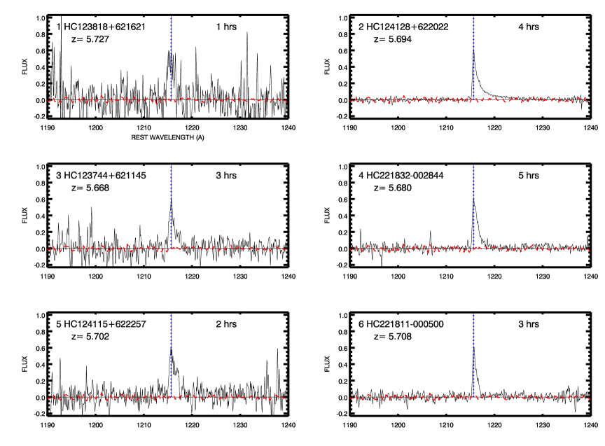
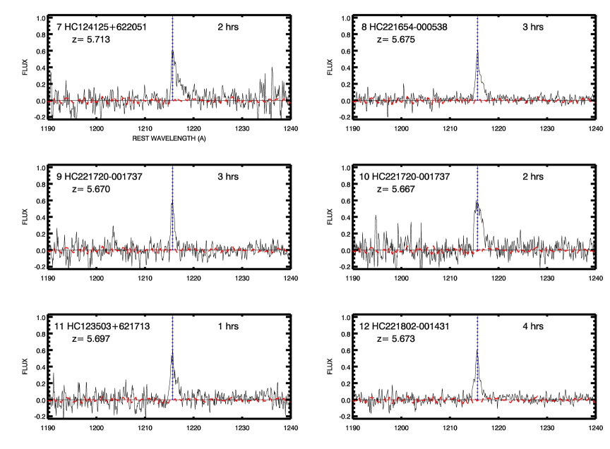
Figure A2.— Spectra of the spectroscopically confirmed $z=5.7$ Ly$\alpha$ emitter sample. For each object we show the spectrum (black) compared with the average spectral shape of the entire sample (red dashed). The blue dotted line shows the position of the spectrum peak, which we use to define the redshift. The name of the object and its redshift is given in the upper left, and the exposure time in hours is given in the upper right.

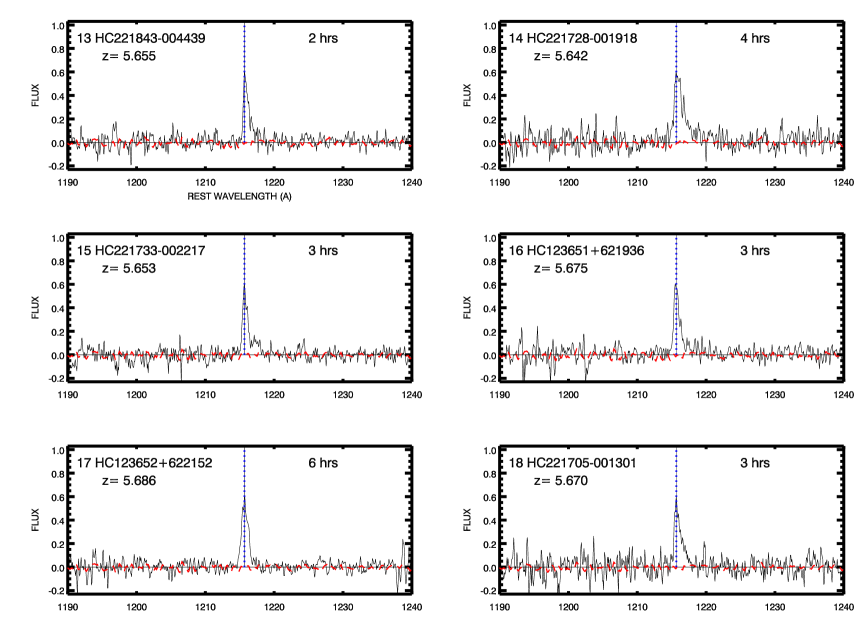
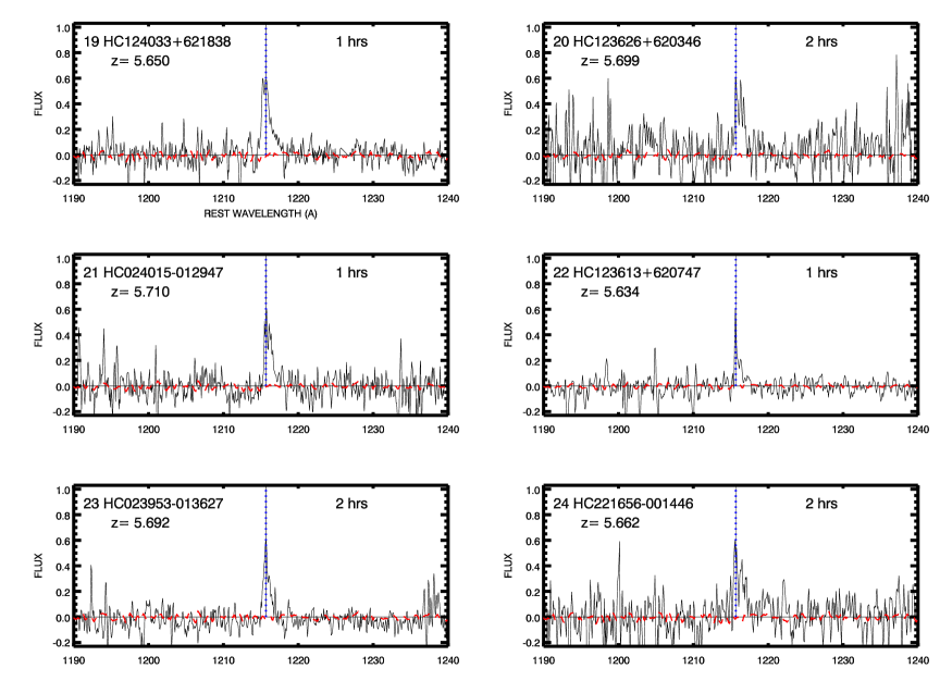
Figure A2.— Spectra of the spectroscopically confirmed $z=5.7$ Ly$\alpha$ emitter sample (continued).

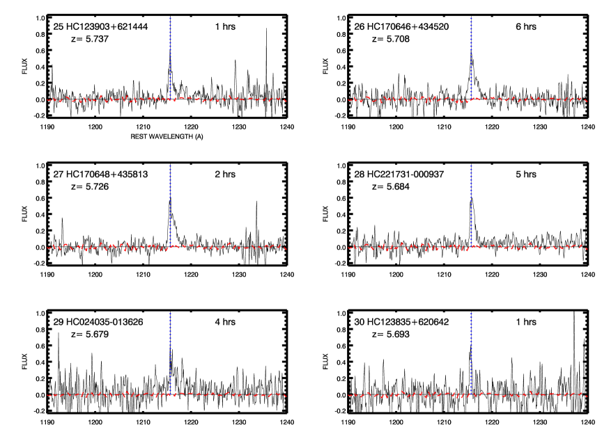
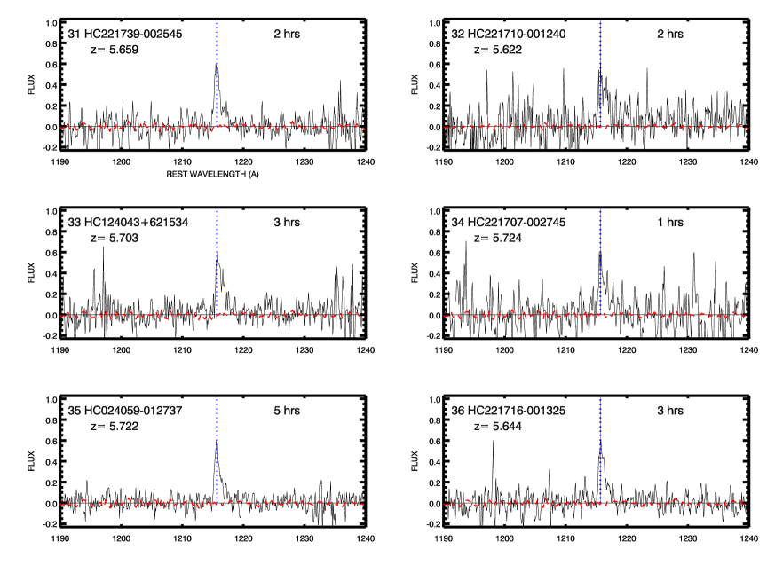
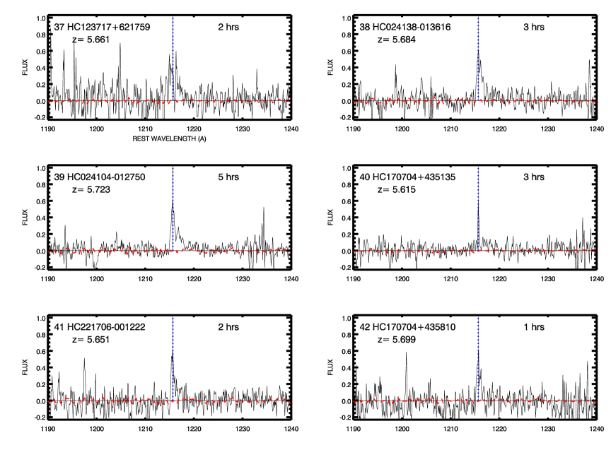
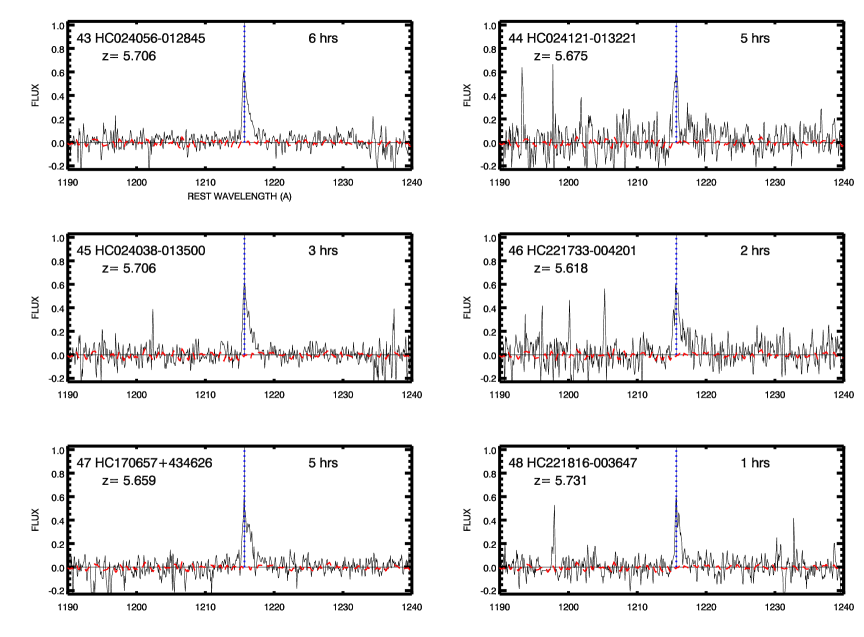
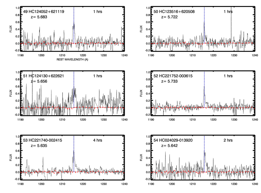
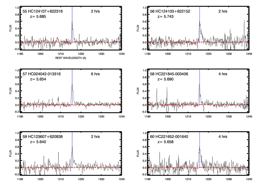
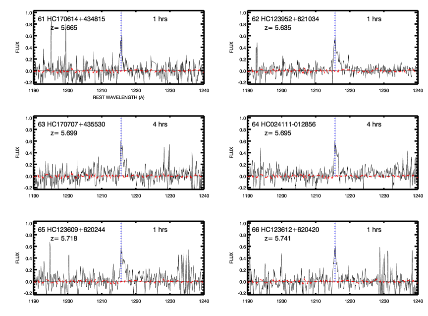
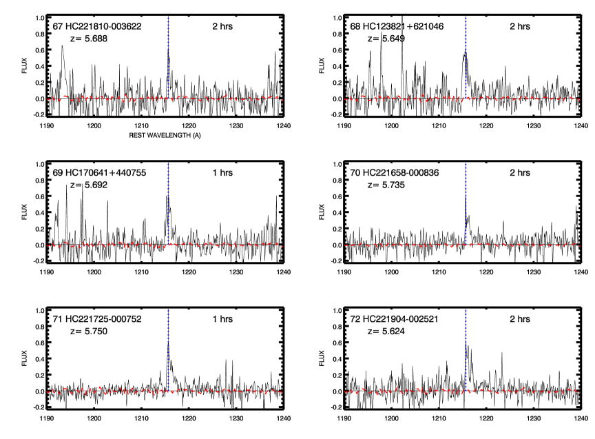
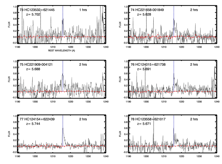
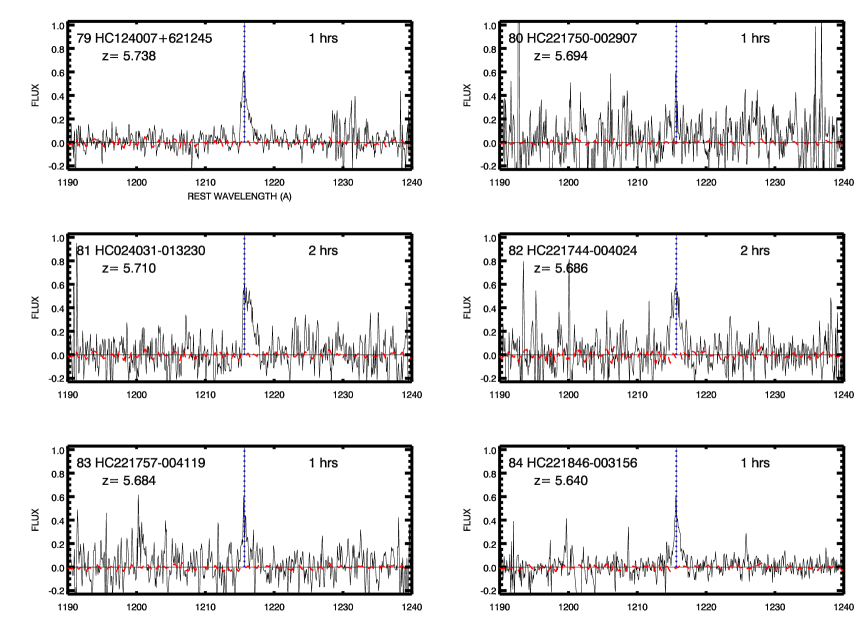
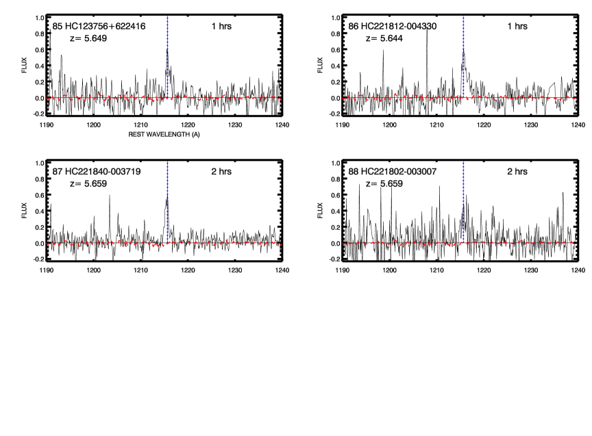
Figure A2.— Spectra of the spectroscopically confirmed $z=5.7$ Ly$\alpha$ emitter sample (continued).

Figure A2.— Spectra of the spectroscopically confirmed $z=5.7$ Ly$\alpha$ emitter sample (continued).

Figure A2.— Spectra of the spectroscopically confirmed $z=5.7$ Ly$\alpha$ emitter sample (continued).

Figure A2.— Spectra of the spectroscopically confirmed $z=5.7$ Ly$\alpha$ emitter sample (continued).

Figure A2.— Spectra of the spectroscopically confirmed $z=5.7$ Ly$\alpha$ emitter sample (continued).

Figure A2.— Spectra of the spectroscopically confirmed $z=5.7$ Ly$\alpha$ emitter sample (continued).

Table 6$z=6.5$ Ly$\alpha$ Emitters

Number	Name	R.A.	Decl.	$N$	$z$	Redshift	Expo	Qual	FWHM	Log(L)
		(J2000)	(J2000)	(AB)	(AB)		(hrs)		Å	erg/s
(1)	(2)	(3)	(4)	(5)	(6)	(7)	(8)	(9)	(10)	(11)
1	HC221741-003134	334.42105	0.5262219	$24.01$	$26.60$	6.5008	2	1	$1.50\pm 0.18$	43.28
2	HC170716+435039	256.81799	43.84438	$24.06$	$26.27$	6.5272	1	1	$0.98\pm 0.11$	43.29
3	HC221725-001119	334.35703	0.1886940	$24.12$	$25.20$	6.5142	2	1	$0.69\pm 0.03$	43.22
4	HC023954-013332	39.978001	-1.559111	$24.24$	$25.18$	6.5587	6	1	$0.76\pm 0.07$	43.41
5	HC221742-001808	334.42896	0.3023610	$24.36$	$26.15$	6.4692	3	1	$0.80\pm 0.08$	43.20
6	HC221749-004825	334.45700	0.8070280	$24.50$	$27.33$	6.4903	1	1	$0.83\pm 0.10$	43.09
7	HC221827-004727	334.61499	0.7909169	$24.53$	$27.81$	6.5036	1	1	$0.73\pm 0.03$	43.05
8	HC221831-004012	334.63306	0.6700829	$24.80$	$26.53$	6.5683	2	1	$1.16\pm 0.14$	43.28
9	HC221848-004353	334.70294	0.7315830	$24.81$	$27.87$	6.5232	2	1	$0.95\pm 0.11$	42.95
10	HC124215+621729	190.56500	62.29150	$24.84$	$27.21$	6.5140	1	1	$0.88\pm 0.12$	42.94
11	HC123512+621911	188.80232	62.31977	$24.87$	$27.04$	6.4975	2	3	$0.55\pm 0.04$	42.92
12	HC124001+621946	190.00801	62.32960	$24.95$	$-26.28$	6.5121	1	2	$0.85\pm 0.12$	42.88
13	HC221823-004631	334.59802	0.7754439	$25.01$	$26.40$	6.4836	1	2	$0.78\pm 0.10$	42.90
14	HC221738-000909	334.41000	0.1526670	$25.01$	$27.41$	6.4811	2	1	$0.61\pm 0.03$	42.87
15	HC023939-013451	39.914791	-1.581028	$25.04$	$28.21$	6.5309	3	1	$0.86\pm 0.09$	42.90
16	HC024055-014315	40.229206	-1.721000	$25.07$	$-27.52$	6.4749	2	1	$0.93\pm 0.10$	42.91
17	HC221801-002220	334.50806	0.3722780	$25.24$	$99.20$	6.5360	2	3	$0.49\pm 0.07$	42.81
18	HC024121-012300	40.341000	-1.383417	$25.26$	$26.45$	6.5051	4	1	$0.76\pm 0.08$	42.76
19	HC024134-013642	40.394211	-1.611778	$25.26$	$26.70$	6.4680	3	1	$0.85\pm 0.09$	42.86
20	HC221733-004304	334.39102	0.7177780	$25.27$	$101.3$	6.5726	1	3	$0.28\pm 0.09$	43.09
21	HC023949-013121	39.956711	-1.522667	$25.42$	$25.35$	6.5640	2	1	$0.76\pm 0.08$	42.99
22	HC024004-012252	40.017708	-1.381278	$25.47$	$26.37$	6.5024	1	1	$0.43\pm 0.02$	42.62
23	HC023939-013432	39.914417	-1.575667	$25.61$	$-27.12$	6.5485	2	2	$0.44\pm 0.03$	42.76
24	HC024014-012414	40.060917	-1.403972	$25.65$	$26.33$	6.5454	1	2	$0.36\pm 0.03$	42.71
25	HC221858-004553	334.74194	0.7649999	$25.67$	$101.3$	6.5556	2	1	$0.87\pm 0.12$	42.81
26	HC024001-014100	40.007500	-1.683388	$25.68$	$-25.91$	6.5444	1	1	$0.75\pm 0.11$	42.72
27	HC023927-013523	39.863293	-1.589833	$25.70$	$27.47$	6.4497	3	1	$0.50\pm 0.08$	42.73

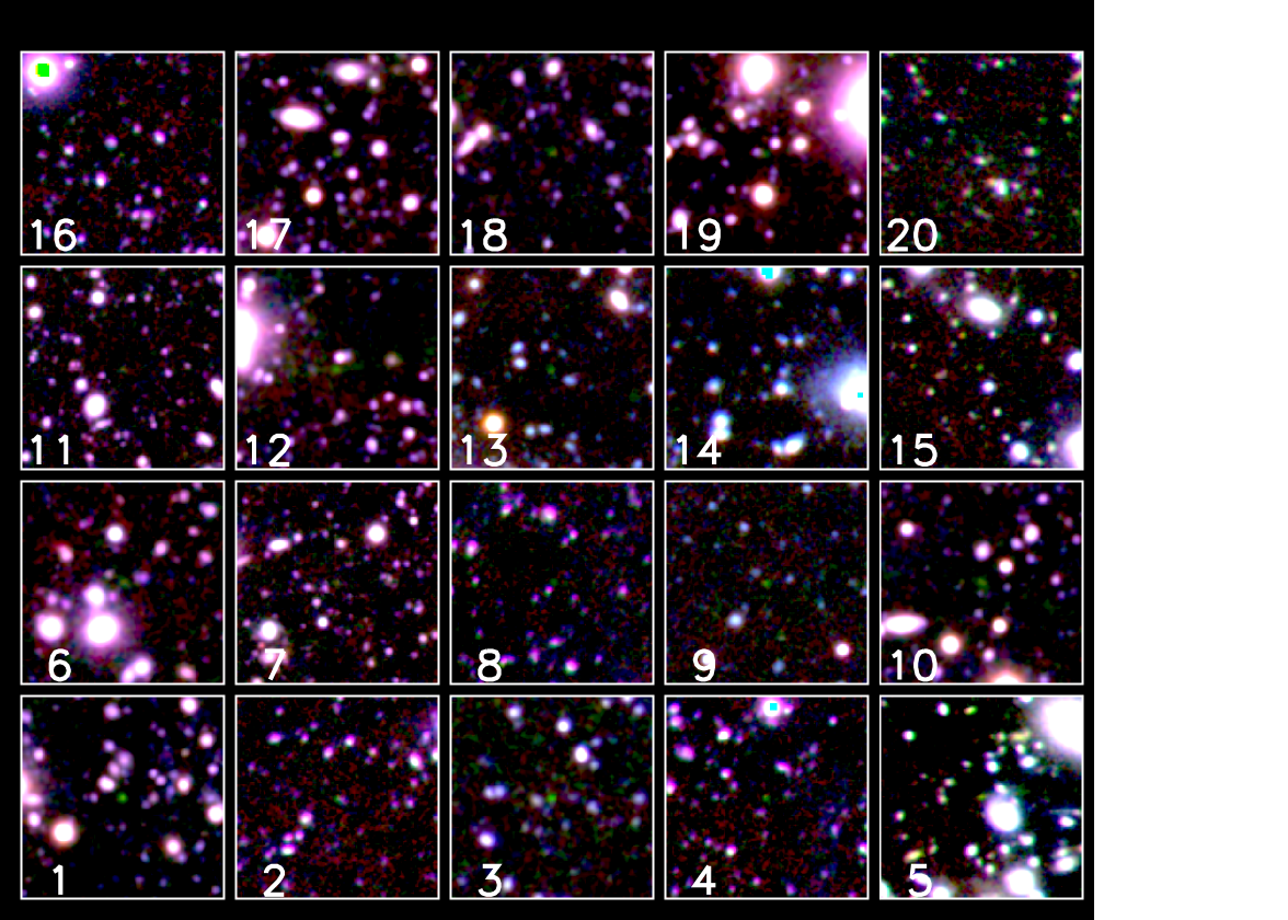
Figure A3.— Images of the spectroscopically confirmed $z=6.5$ Ly$\alpha$ emitter sample. For each object we show a $40^{\prime\prime}$ thumbnail around the emitter with blue=$I$-band, green=F912 narrowband, and red=$z$-band. The emitter appears as a green object at the center of the thumbnail. The numerical label corresponds to the number in Table A3 and Figure A3.

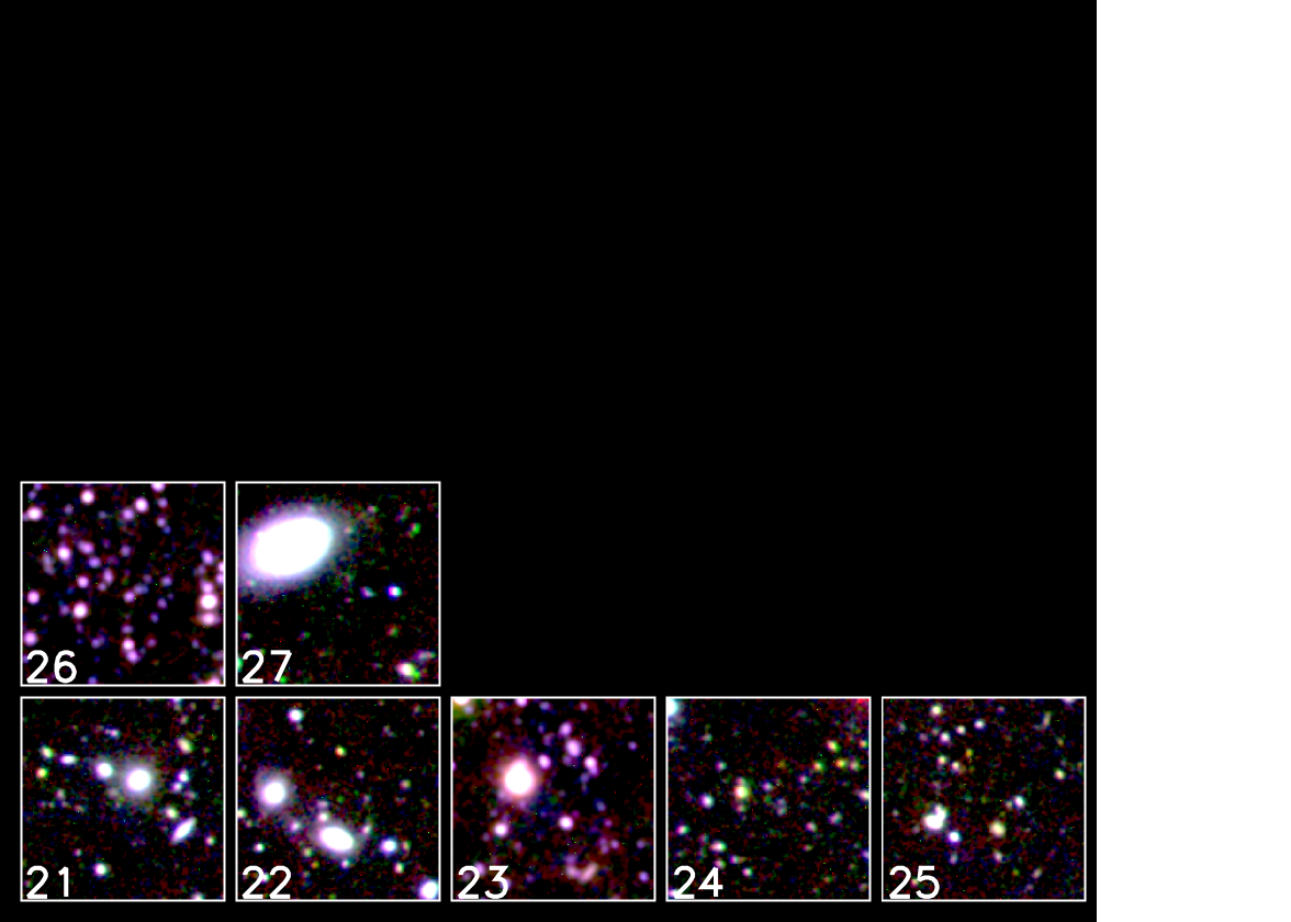
Figure A3.— Images of the spectroscopically confirmed $z=6.5$ Ly$\alpha$ emitter sample (continued).

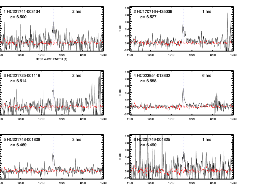
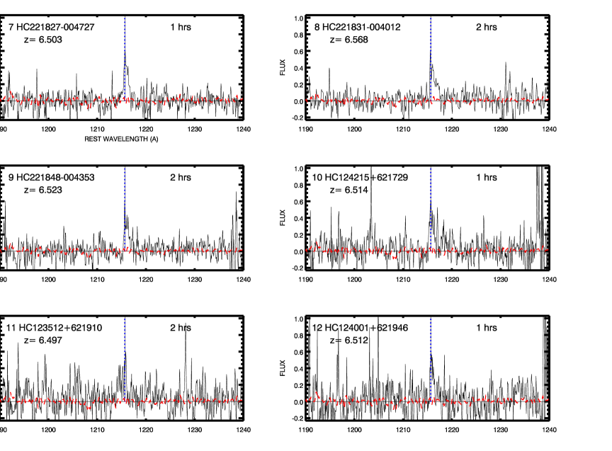
Figure A4.— Spectra of the spectroscopically confirmed $z=6.5$ Ly$\alpha$ emitter sample. For each object we show the spectrum (black) compared with the average spectral shape of the entire sample (red dashed). The blue dotted line shows the position of the spectrum peak, which we use to define the redshift. The name of the object and its redshift is given in the upper left, and the exposure time is given in hours in the upper right.

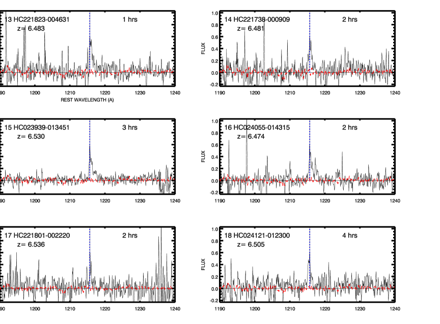
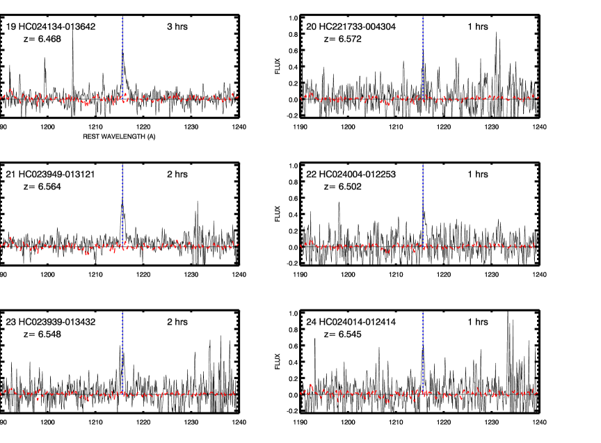
Figure A4.— Spectra of the spectroscopically confirmed $z=6.5$ Ly$\alpha$ emitter sample (continued).

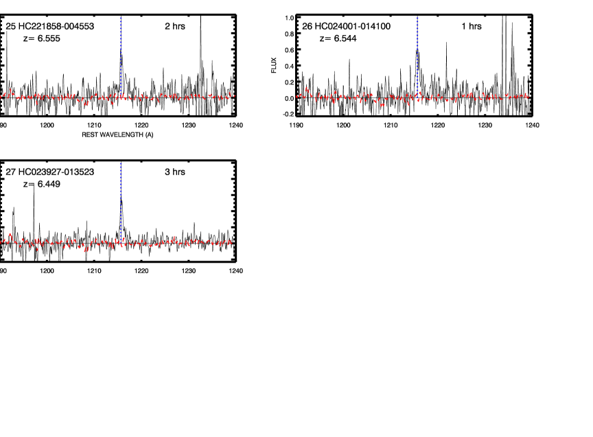
Figure A4.— Spectra of the spectroscopically confirmed $z=6.5$ Ly$\alpha$ emitter sample (continued).

Table 7$z=6.5$ Ly$\alpha$ Emitters (GOODS-N)

Number	Name	R.A.	Decl.	$N$	$z$	Redshift	Expo	Qual	FWHM
		(J2000)	(J2000)	(AB)	(AB)		(hrs)		(Å)
(1)	(2)	(3)	(4)	(5)	(6)	(7)	(8)	(9)	(10)
1	HC123725+621227	189.35800	62.20769	$23.83$	$-28.80$	6.5593	5	1	$0.77\pm 0.06$
2	HC123602+621404	189.00943	62.23466	$24.85$	$-26.84$	6.5610	2	1	$0.70\pm 0.10$
3	HC123637+621022	189.15700	62.17283	$25.37$	$-26.27$	6.5428	2	3	$0.77\pm 0.11$

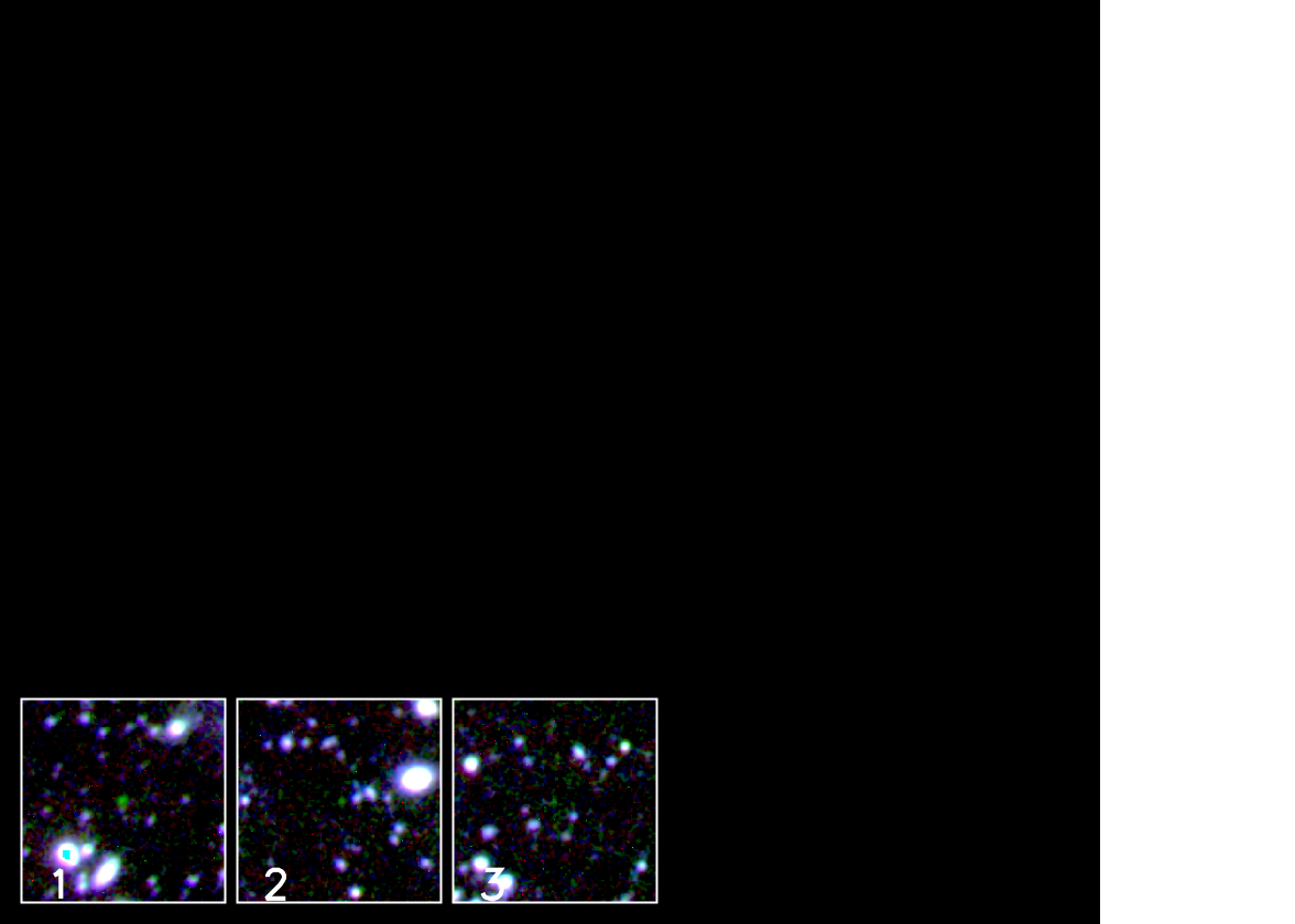
Figure A5.— Images of the spectroscopically confirmed $z=6.5$ Ly$\alpha$ emitter sample in the GOODS-N. For each object we show a $40^{\prime\prime}$ thumbnail around the emitter with blue=$I$-band, green=F921 narrowband, and red=$z$-band. The emitter appears as a green object at the center of the thumbnail. The numerical label corresponds to the number in Table A4 and Figure A6.

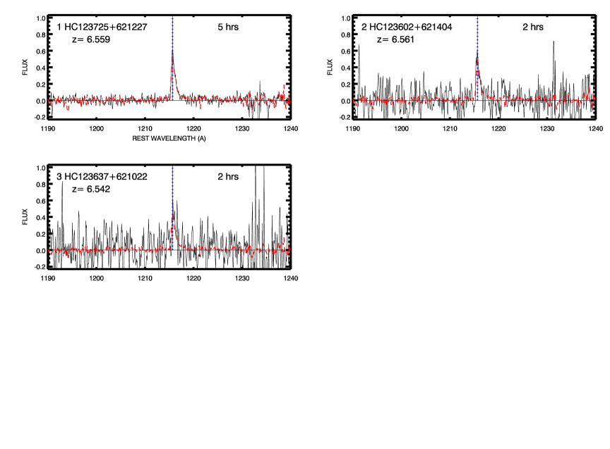
Figure A6.— Spectra of the spectroscopically confirmed $z=6.5$ Ly$\alpha$ emitter sample. For each object we show the spectrum (black) compared with the average spectral shape of the entire sample (red dashed). The blue dotted line shows the position of the spectrum peak, which we use to define the redshift. The name of the object and its redshift is given in the upper left, and the exposure time in hours is given in the upper right.

References

- (1)
- (2) Ajiki, M. et al. 2003. AJ, 126, 2091
- (3)
- (4) Bertin, E., & Arnouts, S. 1996, A&AS, 117, 393
- (5)
- (6) Bouwens, R. J., et al. 2003, ApJ, 595, 589
- (7)
- (8) Bunker, A. J., Stanway, E. R., Ellis, R. S., McMahon, R. G., & McCarthy, P. J. 2003, MNRAS, 342, L47
- (9)
- (10) Capak, P., et al. 2004, AJ, 127, 180
- (11)
- (12) Cowie, L. L., Barger, A. J., & Hu, E. M. 2010, ApJ, 711, 928
- (13)
- (14) Cowie, L. L., & Hu, E. M. 1998, AJ, 115, 1319
- (15)
- (16) Dickinson, M., et al. 2003, ApJ, 600, 99
- (17)
- (18) Dijkstra, M., & Wyithe, J. S. B. 2010, MNRAS, submitted (arXiv:1004.2490)
- (19)
- (20) Dijkstra, M., Wyithe, J. S. B., & Haiman, Z. 2007, MNRAS, 379, 253
- (21)
- (22) Faber, S. M. et al. 2003, Proc. SPIE, 4841, 1657
- (23)
- (24) Finkelstein, S. L., Rhoads, J. E., Malhotra, S., Pirzkal, N., & Wang, J. 2007, ApJ, 660, 1023
- (25)
- (26) Gnedin, N. Y., & Prada, F. 2004, ApJ, 608, L88
- (27)
- (28) Gronwall, C. et al. 2007, ApJ, 667, 79
- (29)
- (30) Haiman, Z., & Cen, R. 2005, ApJ, 623, 627
- (31)
- (32) Hu, E. M., & Cowie, L. L. 2006, Nature, 440, 1145
- (33)
- (34) Hu, E. M., Cowie, L. L., Capak, P., Hayashino, T., & Komiyama, Y. 2004, AJ, 127, 563 (H04)
- (35)
- (36) Hu, E. M., Cowie, L. L., & Kakazu, Y. 2007, Highlights of Astronomy, Volume 14, p.252
- (37)
- (38) Hu, E. M., Cowie, L. L., & McMahon, R. G. 1999, in ASP Conf. Ser. 193, The Hy Redshift Universe, ed. A. J. Bunker & W. J. M. van Breugel (San Francisco: ASP), 554, astro-ph/9911477
- (39)
- (40) Hu, E. M., Cowie, L. L, McMahon, R. G., Capak, P., Iwamuro, F., Kneib, J.-P., Maihara, T., & Motohara, K. 2002, ApJ, 568, L75 (erratum 576, L99)
- (41)
- (42) Iwata, I., et al. 2003, PASJ, 55, 415
- (43)
- (44) Kakazu, Y., Cowie, L. L., & Hu, E. M. 2007, ApJ, 668, 853
- (45)
- (46) Kashikawa, N., et al. 2006, ApJ, 648, 7
- (47)
- (48) Kunth, D., Leitherer, C., Mas-Hesse, J. M., Östlin, G., & Petrosian, A. 2003, ApJ, 597, 263
- (49)
- (50) Landolt, A. U. 1992, AJ, 104, 340
- (51)
- (52) Lehnert, M. D., & Bremer, M. 2003, ApJ, 593, 630
- (53)
- (54) Loeb, A., & Rybicki, G. B. 1999, AJ, 524, 527
- (55)
- (56) Markwardt, C. B. 2009, ASP Conf. Ser., 411, eds. D. Bohlender, P. Dowler, & D. Durand, p.251
- (57)
- (58) Mesinger, A., & Furlanetto, S. R. 2008, MNRAS, 386, 1990
- (59)
- (60) Miyazaki, S., et al. 2002, PASJ, 54, 833
- (61)
- (62) Neufeld, D. A. 1991, ApJ, 370, L85
- (63)
- (64) Oke, J. B. 1990, AJ, 99, 1621
- (65)
- (66) Oke, J. B., et al. 1995, PASP, 107, 375
- (67)
- (68) Oke, J. B., & Gunn, J. E. 1983, ApJ, 266, 713
- (69)
- (70) Ouchi, M., et al. 2008, ApJS, 176, 301
- (71)
- (72) Ouchi, M., et al. 2010, arXiv:1007.2961
- (73)
- (74) Santos, M. R. 2004, MNRAS, 349, 1137
- (75)
- (76) Schaerer, D., & Verhamme, A. 2008, A&A, 480, 369
- (77)
- (78) Schlegel, D. J., Davis, M, and Finkbeiner, D. P. 1998, ApJ, 500, 525
- (79)
- (80) Shimasaku, K., et al. 2006, PASJ, 58, 313
- (81)
- (82) Ouchi, M., et al. 2008, ApJS, 176, 301
- (83)
- (84) Santos, M. R. 2004, MNRAS, 349, 1137
- (85)
- (86) Schaerer, D., & Verhamme, A. 2008, A&A, 480, 369
- (87)
- (88) Schlegel, D. J., Davis, M, and Finkbeiner, D. P. 1998, ApJ, 500, 525
- (89)
- (90) Shimasaku, K., et al. 2006, PASJ, 58, 313
- (91) Ouchi, M., et al. 2008, ApJS, 176, 301
- (92)
- (93) Santos, M. R. 2004, MNRAS, 349, 1137
- (94)
- (95) Schaerer, D., & Verhamme, A. 2008, A&A, 480, 369
- (96)
- (97) Schlegel, D. J., Davis, M, and Finkbeiner, D. P. 1998, ApJ, 500, 525
- (98)
- (99) Shimasaku, K., et al. 2006, PASJ, 58, 313
- (100) Ouchi, M., et al. 2008, ApJS, 176, 301
- (101)
- (102) Santos, M. R. 2004, MNRAS, 349, 1137
- (103)
- (104) Schaerer, D., & Verhamme, A. 2008, A&A, 480, 369
- (105)
- (106) Schlegel, D. J., Davis, M, and Finkbeiner, D. P. 1998, ApJ, 500, 525
- (107)
- (108) Shimasaku, K., et al. 2006, PASJ, 58, 313
- (109)
- (110) Songaila, A. 2004, AJ, 127, 2598
- (111)
- (112) Stanway, E. R., Bunker, A. J., & McMahon, R. G. 2003, MNRAS, 342, 439
- (113)
- (114) Stern, D., & Spinrad, H. 1999, PASP, 111, 1475
- (115)
- (116) Turnshek, D. A., Bohlin, R. C., Williamson II, R. L., Lupie, O. L., Koornneef, J., & Morgan, D.H. 1990, AJ, 99, 1243
- (117)
- (118) van Breukelen, C., Jarvis, M. J., & Venemans, B. P. 2005, MNRAS, 359, 895
- (119)
- (120) Wang, J. X., Malhotra, S., & Rhoads, J. E. 2005, ApJ, 622, L77
- (121)
- (122) Zheng, Z., Cen, R., Trac, H., & Miralda-Escudé, J. 2010, ApJ, 716, 574
- (123)