Limits on Preserving Quantum Coherence using Multi-Pulse Control

Abstract

We explore the physical limits of pulsed dynamical decoupling methods for decoherence control as determined by finite timing resources. By focusing on a decohering qubit controlled by arbitrary sequences of $\pi$-pulses, we establish a non-perturbative quantitative upper bound to the achievable coherence for specified maximum pulsing rate and noise spectral bandwidth. We introduce numerically optimized control “bandwidth-adapted” sequences that saturate the performance bound, and show how they outperform existing sequences in a realistic excitonic-qubit system where timing constraints are significant. As a byproduct, our analysis reinforces the impossibility of fault-tolerance accuracy thresholds for generic open quantum systems under purely reversible error control.

Building on the discovery of spin-echo and multiple-pulse techniques in nuclear magnetic resonance NMR , dynamical decoupling (DD) methods for open quantum systems Vio have become a versatile tool for decoherence control in quantum engineering and fault-tolerant quantum computation. DD involves “open loop” (feedback-free) quantum control based on the application of a time-dependent Hamiltonian which, in the simplest setting, effects a pre-determined sequence of unitary operations (pulses) drawn from a basic repertoire. Physically, DD relies on the ability to access control time scales that are short relative to the correlation time scale of the interaction to be removed. The reduction in decoherence is achieved perturbatively, by ensuring that sufficiently high orders of the error-inducing Hamiltonian are removed. Recently, a number of increasingly powerful pulsed DD schemes have been proposed and validated in the laboratory. Uhrig DD (UDD) sequences Uhrig (2007), for instance, perturbatively cancel pure dephasing in a single qubit up to an arbitrarily high order $n$ while using a minimal number ($n$) of pulses, paving the way to further optimization for given sequence duration Bie ; Uys et al. (2009) and/or specific noise environments noi , to nearly-optimal protocols for generic single-qubit decoherence West et al. (2010). Experimentally, UDD has been employed to prolong coherence time in systems ranging from trapped ions Bie ; Uys et al. (2009); Steane and atomic ensembles Sagi et al. (2010) to spin-based devices Liu , and to enhance contrast in magnetic resonance imaging of tissue War .

In a realistic DD setting, the achievable performance is inevitably influenced by errors due to limited control as well as deviations from the intended decoherence model. Since it is conceivable that both model uncertainty and pulse non-idealities can be largely removed by more accurate system identification and control design, some of these limitations may be regarded as non-fundamental in nature. Composite-pulse Ken and pulse-shaping shape techinques can be used, for instance, to cancel to high accuracy the effects of both systematic control errors and finite-width corrections. We argue, however, that even in a situation where pulses may be assumed perfect and instantaneous, an ultimate constraint is implied by the fact that the rate at which control operations are effected is necessarily finite – as determined by a “minimum switching time” $\tau_{\text{min}}$ for the available control modulation. Our goal in what follows is to rigorously quantify the performance limits to preserving coherence using DD as arising from the sole constraint of finite timing resources.

We focus on the paradigmatic case of a single qubit undergoing pure dephasing due to either a quantum bosonic bath at equilibrium or classical (Gaussian) noise, and controlled through a sequence of instantaneous $\pi$ pulses. While representing an adequate idealization of realistic decoherence control settings Bie ; Uys et al. (2009); Steane ; Sagi et al. (2010); War , this problem is exactly solvable analytically Vio ; Uhrig (2007), enabling rigorous conclusions to be established. Our first result is a non-perturbative lower bound for the minimum decoherence error achievable by any DD sequence subject to a timing constraint $\tau_{\text{min}}$, for noise spectra characterized by a finite spectral bandwidth $\omega_{c}$. Secondly, we show how to generate “bandwidth-adapted” DD sequences that achieve optimum performance over a desired storage time while respecting the pulse-rate constraint, and demonstrate their advantages in a realistic excitonic qubit. Conceptually, our analysis highlights connections between DD theory and complex analysis of polynomials, and provides further insight into the fundamental capabilities and limitations of open-loop non-dissipative quantum control.

Control setting.— Our target system is a single qubit whose dephasing dynamics in the quantum regime is described by a diagonal spin-boson Hamiltonian of the form $H=H_{S}\otimes I_{B}+H_{SB}+I_{S}\otimes H_{B}$, with $H_{S}=\omega S_{z}$ and

$$H_{SB}=S_{z}\otimes\sum_{k}(g_{k}b_{k}+g_{k}^{\ast}b_{k}^{\dagger}),\quad H_{B}=\sum_{k}\omega_{k}b_{k}^{\dagger}b_{k}.$$

Here, $I_{S(B)}$ denote the identity operator on the system (bath), $S_{z}=\hbar\sigma_{z}/2$ is the spin operator along the quantization axis, and $b_{k}$ ($b_{k}^{\dagger}$) are canonical ladder operators for the $k$th bosonic mode, characterized by a frequency $\omega_{k}$ and coupling strength $g_{k}$. If the bath is initially at thermal equilibrium at temperature $1/(k_{B}\beta)$, its influence on the qubit dynamics is encapsulated by the spectral density function $I(\omega)\equiv\!\!\sum_{k}|g_{k}|^{2}\delta(\omega-\omega_{k})$. Without loss of generality, we shall assume that $I(\omega)$ decays to zero beyond a finite ultraviolet cutoff $\omega_{c}$.

DD over an evolution interval $[0,T]$ is achieved by applying a train of $n$ instantaneous $\pi$ pulses (each implementing a Pauli $\sigma_{x}$ operator) at times $\{t_{j}\}$, where $0<t_{1}<\ldots<t_{n}<T$, and we also let $t_{0}\equiv 0$ and $t_{n+1}\equiv T$. While keeping the number of pulses $n$ to a minimum may be desirable for various practical reasons, neither $n$ nor the resulting sequence duration need to be constrained a priori. An arbitrary long duration $T$ may, in fact, be needed for quantum memory. In contrast, infinite pulse repetition rates are both fundamentally impossible and undesirable as long as $T>0$. Let the minimum switching time $\tau_{\text{min}}>0$ lower-bound the smallest control time scale achievable by any sequence:

$$\tau\equiv\min(t_{j+1}-t_{j})\geq\tau_{\text{min}},\;\;\;\;j\in\{0,\ldots,n\}.$$ (1)

If the system is initially in a nontrivial coherent superposition of $S_{z}$ eigenstates, its purity in the presence of DD decays with a factor of $\exp(-2\chi_{\{t_{j}\}})$, where the decoupling error $\chi_{\{t_{j}\}}\geq 0$ can be exactly expressed in the following form (see e.g. Eqs. (8c) and (10) in Uhrig (2007)):

$$\chi_{\{t_{j}\}} = \int_{0}^{\infty}\lambda(\omega)\,|f_{\{\tilde{t}_{j}\}}(\omega)|^{2}d\omega,\quad\;\tilde{t}_{j}\equiv\frac{t_{j}}{\tau},\;\;$$ (2)

$$f_{\{\tilde{t}_{j}\}}(\omega) = \sum_{j=0}^{n}(-1)^{j}(e^{i\tilde{t}_{j}\omega\tau}-e^{i\tilde{t}_{j+1}\omega\tau}),$$ (3)

and the “spectral measure” $\lambda(\omega)\equiv 2\coth(\beta\omega/2)I(\omega)/\omega^{2}$. In terms of the rescaled pulse times $\tilde{t}_{j}$, Eq. (1) becomes $\tilde{t}_{j+1}-\tilde{t}_{j}\geq 1$. Physically, Eqs. (2)-(3) can also describe the purity decay resulting from pure dephasing in the semi-classical limit, as due to stochastic fluctuations of the qubit energy splitting and experimentally investigated in Bie ; Uys et al. (2009); Sagi et al. (2010). In this case, $H_{SB}\equiv 0$ and $H_{S}=[\omega+\xi(t)]S_{z}$, where $\xi(t)$ is a Gaussian random variable with a power spectrum $S(\omega)$ cyw . In order to evaluate $\chi_{\{t_{j}\}}$, it suffices to redefine $\lambda(\omega)=S(\omega)/2\pi\omega^{2}$. The objective of DD is to minimize $\chi_{\{t_{j}\}}$. Our main problem then directly ties to the following: Given the fundamental constraint of Eq. (1), what is a lower bound on $\chi_{\{t_{j}\}}$?

Non-perturbative performance bound.— A lower bound on $\chi_{\{t_{j}\}}$ can be obtained by restricting the integral in Eq. (2) to a finite range $[0,\omega_{c}]$, with a tight bound ensuing if $\omega_{c}$ coincides with the spectral cutoff in either $I(\omega)$ or $S(\omega)$. We separate the dependencies of $\chi_{\{t_{j}\}}$ upon the timings and the spectral measure $\lambda(\omega)$ by applying Cauchy’s inequality to the functions $\lambda^{1/2}|f|$ and $\lambda^{-1/2}$:

$$\chi_{\{t_{j}\}}\geq\frac{1}{M_{\{\lambda\}}}\Big{(}\!\int_{0}^{\omega_{c}}\!\!\!\!|f_{\{\tilde{t}_{j}\}}(\omega)|d\omega\!\Big{)}^{2},\ M_{\{\lambda\}}\equiv\!\!\int_{0}^{\omega_{c}}\!\!\!\!\frac{d\omega}{\lambda(\omega)}.$$ (4)

Thus, the integral $\int_{0}^{\omega_{c}}|f_{\{\tilde{t}_{j}\}}(\omega)|d\omega$, which is the $L_{1}$-norm of the “filter function” $f_{\{\tilde{t}_{j}\}}$ over $[0,\omega_{c}]$, determines a worst-case lower bound on $\chi_{\{t_{j}\}}$ for all spectral densities $\lambda(\omega)$ for which the integral defining $M_{\{\lambda\}}$ is finite.

Interestingly, upon letting $e^{i\omega\tau}\equiv z\in{\mathbb{C}}$ in Eq. (3), the function $f_{\{\tilde{t}_{j}\}}(\omega)$ takes the form of a complex “polynomial” $P_{\{\tilde{t}_{j}\}}(z)$ with non-integer exponents. Such Müntz polynomials have been studied in the mathematical literature, and a plethora of results (and conjectures) exist on their associated norm inequalities, zeroes, and multiplicities Borwein and Erdélyi (1995). The (now resolved) Littlewood conjecture in harmonic analysis Nazarov (1996) may be invoked, in particular, to lower-bound the $L_{1}$-norm of $f_{\{\tilde{t}_{j}\}}$:

$$\chi_{\{t_{j}\}}\geq\frac{\omega_{c}^{2}}{M_{\{\lambda\}}}\,C(\log n)^{2},\quad\text{if }\;\omega_{c}\tau>2\pi,$$ (5)

with $C=O(1)$. Also note that, regardless of $\omega_{c}\tau$, an upper bound follows immediately from Eq. (2): $\chi_{\{t_{j}\}}\leq m_{\{\lambda\}}n^{2}$, where $m_{\{\lambda\}}\equiv\int_{0}^{\infty}\lambda(\omega)d\omega$. Eq. (5) implies that in the “slow-control” regime where $\omega_{c}\tau>2\pi$, the DD error worsens when more pulses are applied, and coherence may be best preserved by doing nothing. This reinforces how sufficiently fast modulation time scales are essential for achieving decoherence reduction, as we discuss next.

The “fast-control” regime ($\omega_{c}\tau<2\pi$) is implicit in perturbative DD treatments, where the filter function $f_{\{\tilde{t}_{j}\}}(\omega)$ is chosen to have a Taylor series that starts at $(\omega\tau)^{m}$, so that $\chi_{\{t_{j}\}}$ remains small for sufficiently small values of $\omega_{c}\tau$. While this perturbative approach has been used for designing efficient DD schemes, it cannot lead to a lower bound on the attainable DD error in the presence of a timing constraint. Consider for example UDD_n sequences, in which case $t_{j}=T\sin^{2}[\pi j/(2n+2)]$ for $j=1,\cdots,n$, and $\tau\equiv t_{1}$. If $\tau$ is kept fixed, increasing $n$ is only possible at the expense of lengthening the total duration as $T(n)=\mathcal{O}[\tau n^{2}]$. Irrespective of the fact that perturbatively the error scales as $\mathcal{O}[(\omega_{c}\tau)^{n}]$, it carries a prefactor that grows too fast with $n$, eventually causing the perturbative description to break down Uhrig and Lidar (2010); Hodgson2009 .

A non-perturbative lower bound may be established by directly mapping the $L_{1}$-norm integral of $f_{\{\tilde{t}_{j}\}}$ to the size of the corresponding Müntz polynomial $P_{\{\tilde{t}_{j}\}}(z)$ over an arc of the unit circle of length $\omega_{c}\tau$. Theorem 2.2 in Erdélyi et al. , in conjunction with Eq. (4), then implies:

$$\chi_{\{t_{j}\}}\geq\frac{1}{M_{\{\lambda\}}\tau^{2}}\,ce^{-a/(\omega_{c}\tau)},\quad\text{if }\;\omega_{c}\tau<2\pi,$$ (6)

for some numeric constants $c$ and $a$ independent of $\tau$, $\omega_{c}$, and $\{t_{j}\}$. The bound in Eq. (6) is strictly positive for spectral measures of compact support. That it cannot be obtained by perturbative methods is manifest from the fact that it describes an essential singularity in $\omega_{c}\tau$.

It is worth to further interpret Eq. (6) in the light of existing results. If the control rate is identified as the key resource that DD leverages for removing errors, a zero lower bound on $\chi_{\{t_{j}\}}$ would allow, in principle, arbitrarily high DD accuracy to be achieved by using sufficiently long sequences with a fixed $\tau_{\text{min}}$ – that is, in analogy with fault-tolerant quantum computation PreskillRel , with a constant resource overhead relative to the noise-free case. Historically, the impossibility of reliable computation with a constant blow-up in resources (circuit depth) was established in Dorit in the broader context of noisy reversible circuits, both classical and quantum. Therefore, our results may be taken to reinforce the fundamental limitations of purely unitary quantum error correction, while explicitly characterizing the way in which such limiting performance depends upon the physical parameters.

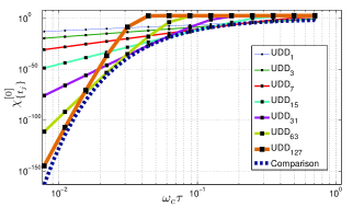
Figure 1: (Color online) Decoupling error for UDD_n sequences vs. $\omega_{c}\tau$, for a “flat” spectral measure $\lambda^{[0]}(\omega)\equiv\Theta(\omega-\omega_{c})$. The comparison curve denotes the general lower bound, Eq. (6), evaluated for $a=3$, $c=1/2$, chosen to approximate a fit.

Achieving the performance bound.— Note that the minimum switching time $\tau_{\text{min}}$ enters Eq. (6) naturally, whereas both the total duration $T$ and pulse number $n$ are markedly absent from it. Thus interestingly, if the bound can be achieved, it should be possible to do so irrespective of how long $T$, provided that $n$ is unconstrained. We can show that the error associated with UDD sequences, $\chi^{\text{UDD}}_{n}$, saturates the fundamental limit in Eq. (6) in functional form although not necessarily in absolute sense (see also Fig. 1). This follows from noting that an upper bound to $\chi^{\text{UDD}}_{n}$ in the presence of a hard spectral cutoff may be obtained from an upper bound to $|f^{\text{UDD}}_{n}(\omega)|$, by tailoring $n$ to the bandwidth, $n\equiv n_{0}\approx 1/(e^{2}\omega_{c}\tau)$ (see Remark 2.6 in Erdélyi et al. ). This yields:

$$\chi^{\text{UDD}}_{n}\leq m_{\{\lambda\}}\cdot\max_{\omega\in[0,\omega_{c}]}|f^{\text{UDD}}_{n_{0}}(\omega)|^{2}\leq\frac{m_{\{\lambda\}}}{\omega_{c}\tau}c^{\prime}e^{-a^{\prime}/(\omega_{c}\tau)},$$

where $c^{\prime}=2/(\pi e^{2}),\,a^{\prime}={2}/{e^{2}}$, and a similar functional form as in Eq. (6) is manifest. With $\tau\equiv t_{1}\equiv\tau_{\text{min}}$ fixed, the duration $T$ of the “tailored UDD_n” sequences scales as $\mathcal{O}[1/(\omega_{c}^{2}\tau_{\text{min}})]$, and the longest allowed $\tau$-value that results in coherence improvement scales as $1/(n\omega_{c})$. Thus, UDD provides no guarantee that the error reaches its absolute minimum and accessing the required $\tau$ becomes increasingly harder as $T$ grows. This motivates searching for DD sequences that can operate beyond the perturbative regime and retain their efficacy over the broadest range possible, up to $1/(n\omega_{c})\lesssim\tau\lesssim 1/\omega_{c}$.

Various optimized DD strategies have been investigated for the qubit-dephasing setting under consideration. In “locally optimized” (LO) DD Bie , optimal pulse timings are determined via direct minimization of the error $\chi_{\{t_{j}\}}$ for a fixed target storage time $T$, whereas in “optimized noise filtration” (OF) DD, only the integral of the filter function is minimized Uys et al. (2009) (see also noi for a noise-adapted perturbative approach). While LODD/OFDD can access regimes where perturbative approaches are not efficient, they focus on matching the total sequence duration $T$ as the fundamental constraint. However, this may fail to produce a satisfactory control solution if the timing constraint imposed by Eq. (1) is significant.

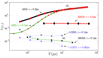
Figure 2: (Color online) Decoupling error for BADD (dashed), LODD (dotted), and UDD (solid) sequences vs. total duration $T$ with the minimum interval $\tau$’s indicated, for a dephasing exciton qubit operating at temperature $77$K (see text). The search space for BADD and LODD covers up to $n=100$ pulses, whereas for UDD $n\leq 20$. See the Appendix for further detail and a comparison between different pulse timing patterns.

To guarantee that such a fundamental limitation is obeyed, we introduce optimized bandwidth-adapted DD (BADD) sequences where both the minimum switching time and the total time are constrained from the outset, see the Appendix for additional technical detail. We demonstrate the usefulness of BADD by focusing on the exciton qubit analyzed in Hodgson2009 , for which a spin-boson dephasing model with a supra-Ohmic spectral density and a Gaussian cutoff is appropriate, $I^{\omega_{c},s}(\omega)=\alpha\omega^{s}\exp(-\omega^{2}/\omega_{c}^{2})$ with $s=3$, $\alpha\approx 1.14\times 10^{-26}$s², $\omega_{c}\approx 3\,\text{rad}\,\text{ps}^{-1}$, and the need to avoid unwanted excitation of higher-energy levels enforces a timing constraint $\tau_{\text{min}}\approx 0.1$ ps pulsew . The results are summarized in Fig. 2. Besides indicating the inadequacy of perturbative UDD for $T\gtrsim 1$ ps, two main features emerge. First, as predicted by Eq. (6), the minimum error achievable by BADD is mainly dictated by $\tau$, largely independently of the total time $T$. Second, LODD performance is fairly sensitive to the timing constraint: for a fixed $T$ ($10$ ps in Fig. 2), “softening” the constraint selects LODD sequences that outperform BADD, the opposite behavior being seen if the constraint on the intended $\tau$ is ”hardened”. Thus, a BADD protocol effectively optimizes over a set of LODD sequences where the timing constraint is only approximately met, consistent with intuition.

In practice, an important question is whether the performance of a DD scheme is robust against uncertainties in the underlying spectral measure: in particular, sequences adapted to a presumed $\omega_{c}\tau_{\text{min}}$ need not be adequate for the actual $\omega_{c}^{\prime}\tau_{\text{min}}$. Some illustrative results are depicted in Fig. 3 for sequences subject to the same timing constraint, but applied to a setting where $\omega_{c}^{\prime}\neq\omega_{c}$. Clearly, a smaller cutoff $\omega_{c}^{\prime}$ leads to smaller decoherence, but much more so for perturbative UDD sequences. Expectedly, the knowledge of the spectral density explicitly assumed in generating BADD and LODD results in far better coherence compared to OFDD and UDD, especially when this knowledge is precise ($\omega_{c}^{\prime}/\omega_{c}=1$) or overestimates the cutoff. Comparatively, BADD sequences appear to be more robust than LODD sequences when the cutoff is underestimated.

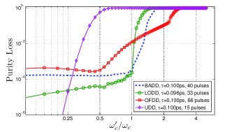
Figure 3: (Color online) Purity loss, $1-e^{-2\chi_{\{t_{j}\}}}$, vs. actual over presumed cutoff, $\omega_{c}^{\prime}/\omega_{c}$, for the supra-Ohmic Gaussian spectral density ($s=3$) corresponding to the exciton qubit. All sequences are adapted to $T\approx 10$ps, $\tau\approx 0.1$ps. Varying the “actual” power law of the noise to $s=4$ and $s=2$ resulted in a qualitatively similar behavior (data not shown).

Discussion.— Our mathematical description has relied on the solvability of the dephasing spin-boson model in the limit of instantaneous control pulses, however we expect similar timing-induced lower bounds to exist under more general conditions. In principle, non-Gaussian classical dephasing such as random telegraph noise could be addressed based on the exact solution presented in Kitajima et al. (2010), whereas non-bosonic dephasing models of the form $H_{SB}+H_{B}\equiv S_{z}\otimes B_{z}+B_{0}$, could be tackled by matching the leading-order contributions in $B_{z}$ with the bosonic case studied here. Note, however, that bounded timing resources do not prevent the DD accuracy bound to be zero in special cases – such as “monochromatic” or “non-dynamical” baths ($H_{B}=0$), for both of which the length of the arc appearing in Eq. (6) vanishes. Similarly, “nilpotent” environments, where powers of the bath operators in $H_{SB}$ and $H_{B}$ vanish at some order, allow perturbative DD schemes to achieve perfect decoupling, as perturbation theory becomes exact. For more “adversarial” environments, where $H_{SB}$ is not restricted to but includes single-axis decoherence, similar lower bounds must exist by inclusion. Elucidating the algebraic features responsible for a finite vs. zero performance bound remains an interesting open problem with implications for quantum error correction in general. As opposed to pulsed control scenarios, continuous-time modulation subject to finite energy/bandwidth constraints has also been explored for decoherence control Gordon et al. (2008). Although, even for a purely dephasing qubit, finding the optimal modulation requires solving a non-linear integro-differential equation, it would be interesting to quantify the extent to which the extra freedom afforded by continuous controls may improve the achievable performance lower bounds.

We thank Michael Biercuk, Irene D’Amico, Daniel Lidar, and John Preskill for valuable input. Work supported from the NSF through Grant No. PHY-0903727.

Appendix: BADD Optimization Procedure

The BADD optimization procedure uses the following input: the spectral measure $\lambda(\omega)$ used to characterize the environment (a continuous positive-valued function defined on positive real numbers); the minimum switching time $\tau$ used to constrain the pulse timings (a positive real number); the total duration $T$ of the sequence (a positive real number larger than $\tau$). The output from BADD is the number of pulses $n$ (a positive integer) and the pulse intervals $\{\tau_{j}\}_{j=1}^{n+1}$ (positive real numbers) that yield the smallest decoupling error while satisfying the following two constraints:

$$(1)\;\tau_{j}\geq\tau,\quad\quad(2)\;\sum_{i=1}^{n+1}\tau_{i}=T.$$

Both these constraints are linear in the variable

$$\mathbf{x}^{(n)}:=(\tau_{1},\tau_{2},\cdots,\tau_{n+1}).$$

Also notice that $n$ is always bounded:

$$1\leq n\leq n_{\text{max}}\equiv T/\tau-1$$

The quantity to be minimized is the coherence loss over time $T$, which is given by [see Eqs. (2)-(3) in the main text]:

$$\chi(\mathbf{x})=\int_{0}^{\infty}\lambda(\omega)|f_{\mathbf{x}}(\omega)|^{2}d\omega,$$

where

$$f_{\mathbf{x}}(\omega) = \sum_{j=0}^{n}(-1)^{j}(e^{it_{j}\omega}-e^{it_{j+1}\omega}),$$

$$t_{j} = \sum_{l=1}^{j}\tau_{l}.$$

The optimization problem described by $\chi(\mathbf{x})$ is highly non-linear and involves evaluation of $\chi(\mathbf{x})$, itself an infinite numerical integral. Computationally, we replace the upper limit of infinity on the integral with a parameter $\omega_{\infty}$ chosen such that

$$\int_{0}^{\infty}\lambda(\omega)|f_{\mathbf{x}}(\omega)|^{2}d\omega\approx\int_{0}^{\omega_{\infty}}\lambda(\omega)|f_{\mathbf{x}}(\omega)|^{2}d\omega.$$

In the soft-cutoff exciton qubit example considered in the main text, setting $\omega_{\infty}=5\omega_{c}$ is more than adequate. We use the general-purpose routines of Matlab for evaluation and optimization of $\chi(\mathbf{x})$. In particular, we hard code the form of $\lambda(\omega)$ into a Matlab function and evaluate the integral for $\chi(\mathbf{x})$ using Matlab’s quadv function (recursive adaptive Simpson quadrature). The numeric optimization is performed with the fmincov function (linear constraints, nonlinear objective, and automatically chosen algorithm) with a numerical tolerance of $10^{-6}$ for both the optimal value and the constraint satisfaction. This procedure returns an optimal choice of intervals $\mathbf{x}_{\text{min}}^{(n)}$ and a corresponding minimum error $\chi_{\text{min}}^{(n)}$ for all possible values of $n\in\{1,\cdots,n_{\text{max}}\}$. The minimum of $\{\chi_{\text{min}}^{(n)}\}_{n=1}^{n_{\text{max}}}$ values identifies the BADD optimized solution. The numerical procedure for generating Fig. 2 in the main text takes about 4 hours to finish using 3 parallel jobs each running on a 2.7GHz quad-core cpu.

Figure 4: (Color online) Pictorial comparison between the pulse timing patterns for the BADD and UDD sequences corresponding to $T\approx 10$, $\tau=0.1$ps (points (a) and (b) in Fig. 2 of the main text). Notice how the intervals of the BADD sequence (a) are compressed at the endpoints, but become effectively uniform mid-sequence. This resembles the (analytical) interpolated DD protocol identified in T. E. Hodgson, L. Viola, and I. D’Amico, Phys. Rev. A 81, 062321 (2010).

In addition to the features discussed in the main text, the following qualitative features are worth emphasizing:

• Theoretically, imposing constraints (1)-(2) together makes the search space compact even including the range of possible pulse numbers. Furthermore, Eq. (6) in the main text provides an explicit lower bound on the objective function, independent of the duration $T$ as well as the pulse number. Both these facts provide a solid foundation for the BADD procedure.

• The optimization always returns $\tau_{1}=\tau$, that is, the first interval uses the shortest available pulse interval.

• When $\omega_{c}\tau$ is sufficiently small, the overall BADD timing pattern approaches that of UDD pulse sequences. Conversely, when $\omega_{c}\tau$ is large, the timing pattern approaches a periodic one, consisting of nearly equidistant pulses. This is depicted in Fig. 1 above for a BADD sequence ($n=40$) and a UDD sequence ($n=15$) operating at $\omega_{c}\tau=0.3$, corresponding to the smallest allowed value for the excitonic qubit discussed in the main text.

• Consequently, the optimal number of pulses $n$ approaches $n_{\text{max}}$ when $\tau\omega_{c}$ is large; for smaller $\tau\omega_{c}$ the number of pulses required is smaller than $n_{\text{max}}$.

• The BADD optimized error does not vary significantly with the total time $T$, in line with the expectation that a lower bound on decoupling error does not depend on $T$.

The LODD optimization setting mentioned in the text differs from BADD since it uses $n$ and $T$ as the input (instead of $\tau$ and $T$), and only constraint (2) is imposed in the minimization of the error $\chi(\mathbf{x})$. The OFDD optimization procedure is similar to LODD in this respect, however it uses a specific “flat” spectral measure in which $\lambda(\omega)$ is equal to $1$ for $\omega<\omega_{c}$ and 0 otherwise. That is, OFDD minimizes the integral of the filter function independently of the actual spectral measure $\lambda$, leading to a minimum error which always upper-bounds the one from LODD. As also discussed in the main text, for a given value of $T$ the pulse sequences from BADD and LODD can effectively be matched by comparing them at (almost) equal $\tau$’s. BADD sequences can thus be approximated by searching LODD sequences with different pulse numbers for satisfying the minimum interval condition (1).

References

- (1) E. L. Hahn, Phys. Rev. 80, 580 (1950); U. Haeberlen and J. S. Waugh, Phys. Rev. 175, 453 (1968).
- (2) L. Viola and S. Lloyd, Phys. Rev. A 58, 2733 (1998); L. Viola, E. Knill, and S. Lloyd, Phys. Rev. Lett. 82, 2417 (1999).
- Uhrig (2007) G. S. Uhrig, Phys. Rev. Lett. 98, 100504 (2007).
- (4) M. J. Biercuk et al., Nature 458, 996 (2009); Phys. Rev. A 79, 062304 (2009).
- Uys et al. (2009) H. Uys, M. J. Biercuk, and J. J. Bollinger, Phys. Rev. Lett. 103, 040501 (2009).
- (6) S. Pasini and G. S. Uhrig, Phys. Rev. A 81, 012309 (2010); Y. Pan, Z. Xi, and W. Cui, arXiv:1001.2960.
- West et al. (2010) J. R. West, B. H. Fong, and D. A. Lidar, Phys. Rev. Lett. 104, 130501 (2010).
- (8) D. J. Szwer et al., arXiv:1009.6189.
- Sagi et al. (2010) Y. Sagi, I. Almog, and N. Davidson, Phys. Rev. Lett. 105, 053201 (2010).
- (10) J. Du et al., Nature 461, 1265 (2009).
- (11) E. R. Jenista et al., J. Chem. Phys. 131, 240510 (2009).
- (12) K. R. Brown, A. W. Harrow, and I. L. Chuang, Phys. Rev. A 70, 052318 (2004).
- (13) L. P. Pryadko and G. Quiroz, Phys. Rev. A 77, 012330 (2008); G. S. Uhrig and S. Pasini, New J. Phys. 12, 045001 (2010).
- (14) L. Cywiński et al., Phys. Rev. B 77, 174509 (2008).
- Borwein and Erdélyi (1995) P. B. Borwein and T. Erdélyi, Polynomials and Polynomial Inequalities (Springer Verlag, Berlin, 1995).
- Nazarov (1996) F. L. Nazarov, St. Petersburg Math. J. 7, 265 (1996).
- Uhrig and Lidar (2010) G. S. Uhrig and D. A. Lidar, Phys. Rev. A 82, 012301 (2010).
- (18) T. E. Hodgson, L. Viola, and I. D’Amico, Phys. Rev. B 78, 165311 (2008); Phys. Rev. A 81, 062321 (2010).
- (19) T. Erdélyi, K. Khodjasteh, and L. Viola, arXiv:math.CA/1006.4323.
- (20) J. Preskill, Proc. R. Soc. London A 454, 385 (1998).
- (21) D. Aharonov, M. Ben-Or, R. Impagliazzo, and N. Nisan, arXiv:quant-ph/9611028.
- (22) Typical pulse-widths for this system are on the order of . The analysis in Hodgson2009 shows that treating pulses as instantaneous is accurate (to within per pulse) as long as .
- Kitajima et al. (2010) S. Kitajima, M. Ban, and F. Shibata, J. Phys. A 43, 135504 (2010).
- Gordon et al. (2008) G. Gordon, G. Kurizki, and D. A. Lidar, Phys. Rev. Lett. 101, 010403 (2008).