The UK Infrared Telescope M 33 monitoring project. I. Variable red giant stars in the central square kiloparsec

Abstract

We have conducted a near-infrared monitoring campaign at the UK InfraRed Telescope (UKIRT), of the Local Group spiral galaxy M 33 (Triangulum). The main aim was to identify stars in the very final stage of their evolution, and for which the luminosity is more directly related to the birth mass than the more numerous less-evolved giant stars that continue to increase in luminosity. The most extensive dataset was obtained in the K-band with the UIST instrument for the central $4^{\prime}\times 4^{\prime}$ (1 kpc²) – this contains the nuclear star cluster and inner disc. These data, taken during the period 2003–2007, were complemented by J- and H-band images. Photometry was obtained for 18,398 stars in this region; of these, 812 stars were found to be variable, most of which are Asymptotic Giant Branch (AGB) stars. Our data were matched to optical catalogues of variable stars and carbon stars, and to mid-infrared photometry from the Spitzer Space Telescope. In this first of a series of papers, we present the methodology of the variability survey and the photometric catalogue – which is made publicly available at the Centre de Données astronomiques de Strasbourg (CDS) – and discuss the properties of the variable stars. Most dusty AGB stars had not been previously identified in optical variability surveys, and our survey is also more complete for these types of stars than the Spitzer survey.

1 Introduction

Messier 33 is one of three stereotypical spiral galaxies that inhabit the Local Group. Located in the constellation of Triangulum, it spans about a degree on the sky. Its favourable inclination angle of $56^{\circ}$ makes M 33 a prime subject for the study of the detailed structure and stellar content of a spiral galaxy like our own.

The distance to M 33 has been determined via several methods: Freedman, Wilson & Madore (1991) determined a distance of 850 kpc by using Cepheid-type variables, i.e. a distance modulus $\mu=24.65$ mag, but Scowcroft et al. (2009) revisited this to $\mu=24.53\pm 0.11$ mag. By using RR Lyrae-type variables, Sarajedini et al. (2000) found $\mu=24.84$ mag. Other techniques that have been employed used the tip of the Red Giant Branch (RGB; Rizzi et al. 2007; Galleti, Bellazzini & Ferraro 2004; McConnachie et al. 2004; Tiede, Sarajedini & Barker 2004; Kim et al. 2002), Long-Period Variables (LPVs; Pierce, Jurcević & Crabtree 2000), and detached eclipsing binaries (Bonanos et al. 2006) – the latter, a largely geometric technique, yielded $\mu=24.92\pm 0.12$ mag. U et al. (2009) reviewed these techniques, which result in differences in distance modulus of $\Delta\mu\sim 0.6$ mag, corresponding to an uncertainty in the distance of $\approx 30$%. By using blue (massive) supergiants, U et al. themselves determined $\mu=24.93\pm 0.11$ mag. In this paper we shall adopt $\mu=24.9$ mag.

Tracing stellar populations of a wide range in ages, from as recently formed as 30 Myr ago to as ancient as 10 Gyr, Asymptotic Giant Branch (AGB) stars (Marigo et al. 2008) are exquisite probes of the star formation history of galaxies. With their high luminosity ($\approx 1000$–60,000 L_⊙) and low temperature ($T\sim 3000$–4500 K), AGB stars dominate the appearance of galaxies at near-infrared (near-IR) wavelengths. This is aided further by the low extinction at IR wavelengths compared to that at optical wavelengths. More massive stars, up to $\sim 30$ M_⊙, become red supergiants (RSGs; Levesque et al. 2005; Levesque 2010) and they can be used to trace the more recent star formation history over about 10–30 Myr ago.

Stars at this advanced level of evolution exhibit strong radial pulsations on timescales of typically 150–1500 days (e.g., Wood et al. 1992; Wood 1998; Pierce et al. 2000; Whitelock et al. 2003). As a result of this pulsation AGB stars lose up to 80% of their mass to the interstellar medium (ISM; Bowen 1988; Bowen & Willson 1991; Vassiliadis & Wood 1993; van Loon et al. 1999, 2005), making AGB stars important contributors to chemical enrichment of galaxies; RSGs contribute less in total, but their mass loss sets the conditions within which the ensuing supernova develops (van Loon 2010). The most-evolved AGB stars pulsate in the fundamental mode, which has the largest amplitude, with less-evolved AGB stars and RGB stars pulsating in an overtone with a smaller amplitude (Wood 1999). Though no less powerful, the amplitude of pulsation expressed in terms of magnitude, being a relative scale, diminishes with increasing time-averaged luminosity (Wood et al. 1992; van Loon et al. 2008) making it more difficult to detect the pulsation of RSGs than of lower-luminosity AGB stars (though the photometric errors for RSGs are also smaller).

Detecting variable AGB stars is a powerful tool in reconstructing the star formation history of a galaxy as these stars are in the final stages of their evolution and hence their luminosity is more directly related to their birth mass than that of less-evolved AGB stars that still undergo significant evolution in luminosity.

Various variability surveys have been conducted in M 33, mostly at optical wavelengths and with cadences too short to adequately identify LPVs. Among the most comprehensive monitoring campaigns count those of Hartman et al. (2006), the DIRECT project (Macri et al. 2001; Mochejska et al. 2001a,b), and Sarajedini et al. (2006) who identified 64 RR Lyrae variables. McQuinn et al. (2007), on the other hand, identified variables in M 33 on the basis of five epochs of mid-IR observations performed with the Spitzer Space Telescope.

The main objectives of the project are: to construct the mass function of LPVs and derive from this the star formation history in M 33; to correlate spatial distributions of the LPVs of different mass with galactic structures (spheroid, disc and spiral arm components); to measure the rate at which dust is produced and fed into the ISM; to establish correlations between the dust production rate, luminosity, and amplitude of an LPV; and to compare the in situ dust replenishment with the amount of pre-existing dust. This is Paper I in the series, presenting the methodology used in the monitoring campaign and search for variable stars, the properties of the photometric catalogue of stars in the inner square kpc, and cross-identifications in various other relevant photometric and variability catalogues. Subsequent papers in the series will discuss the galactic structure and star formation history in the inner square kpc (Paper II), the mass-loss mechanism and dust production rate (Paper III), and the extension to a nearly square degree area covering much of the M 33 optical disc (Paper IV).

2 Observations

Observations were made with three of UKIRT’s imagers: UIST, UFTI, and WFCAM. The WFCAM observations cover a much larger part of M 33 and are discussed in Paper IV in this series.

2.1 UIST

Table 1: Log of UIST observations of each of 4 quadrants (“Q”).

Date (y m d)	Q	Filter	Epoch	$t_{\rm int}$ (min)	Airmass
2003 10 06	1	K	1	21	1.49–1.35
2003 10 06	1	J	1	15	1.11–1.08
2003 10 06	2	K	1	21	1.24–1.16
2003 10 06	2	J	1	15	1.08–1.05
2003 11 18	3	K	1	21	1.21–1.30
2004 01 06	3	K	2	21	1.02–1.02
2004 01 06	3	J	1	15	1.05–1.07
2004 01 06	4	K	1	21	1.02–1.03
2004 01 06	4	J	1	15	1.08–1.11
2004 07 25	1	K	2	27	1.22–1.13
2004 07 25	2	K	2	27	1.12–1.07
2004 07 25	3	K	3	27	1.05–1.02
2004 07 26	4	K	2	27	1.05–1.02
2004 09 09	1	K	3	27	1.34–1.21
2004 09 09	2	K	3	27	1.21–1.12
2004 09 09	3	K	4	27	1.09–1.04
2004 09 09	4	K	3	27	1.04–1.02
2004 12 24	1	K	4	27	1.03–1.07
2004 12 24	2	K	4	27	1.07–1.13
2005 01 08	1	J	2	21	1.35–1.49
2005 01 08	2	J	2	21	1.51–1.71
2005 01 18	1	H	1	15	1.03–1.05
2005 01 18	2	H	1	15	1.05–1.07
2005 01 25	3	K	5	27	1.05–1.10
2005 01 25	4	K	4	27	1.11–1.18
2005 02 22	3	K	6	27	1.40–1.62
2005 02 22	4	K	5	27	1.63–1.98
2005 07 04	1	K	5	27	1.63–1.41
2005 07 04	2	K	5	27	1.40–1.26
2005 07 05	3	K	7	27	1.70–1.46
2005 07 05	4	K	6	27	1.45–1.29
2005 07 27	1	K	6	27	1.25–1.15
2005 07 27	2	K	6	27	1.15–1.08
2006 08 08	1	K	7	27	1.27–1.17
2006 08 08	1	J	3	27	1.07–1.03
2006 08 08	2	K	7	27	1.16–1.09
2006 08 08	2	J	3	27	1.03–1.02
2006 08 09	1	H	2	27	1.40–1.26
2006 08 09	2	H	2	27	1.25–1.15
2006 08 09	3	K	8	27	1.12–1.06
2006 08 09	3	H	1	27	1.02–1.02
2006 08 09	4	K	7	27	1.06–1.03
2006 08 09	4	H	1	27	1.02–1.03
2006 08 10	3	J	2	27	1.17–1.10
2006 08 10	4	J	2	27	1.10–1.05
2006 09 06	3	K	9	22	1.42–1.25
2006 09 06	4	K	8	22	1.25–1.14
2006 09 10	1	K	8	22	1.04–1.02
2006 09 10	2	K	8	21	1.02–1.03
2006 10 03	3	K	10	21	1.67–1.48
2006 10 03	4	K	9	21	1.48–1.34
2006 10 04	1	K	9	21	1.66–1.48
2006 10 04	2	K	9	21	1.47–1.34
2006 10 23	1	K	10	21	1.14–1.09
2006 10 23	2	K	10	21	1.09–1.05
2006 10 23	3	K	11	21	1.06–1.09
2006 10 23	4	K	10	21	1.10–1.15
2007 06 18	3	K	12	27	1.53–1.35
2007 07 03	4	K	11	27	1.31–1.20
2007 07 13	2	K	11	27	1.11–1.06
2007 07 25	1	K	11	27	1.05–1.02

The monitoring campaign comprises observations with the UIST imager, of each of four quadrants with slight overlap keeping the unresolved nucleus of M 33 in one of the corners of the field. The approximate centres (slight variations occur due to the absolute pointing accuracy of UKIRT) are respectively ($1^{\rm h}33^{\rm m}47.^{\rm s}0$, $+30^{\circ}38^{\prime}47^{\prime\prime}$), ($1^{\rm h}33^{\rm m}54.^{\rm s}8$, $+30^{\circ}38^{\prime}47^{\prime\prime}$), ($1^{\rm h}33^{\rm m}54.^{\rm s}8$, $+30^{\circ}40^{\prime}27^{\prime\prime}$), ($1^{\rm h}33^{\rm m}47.^{\rm s}0$, $+30^{\circ}40^{\prime}27^{\prime\prime}$), for fields 1, 2, 3 and 4. Observations were made in the K-band (UKIRT filter K98) over the period October 2003 – July 2007. All quadrants were imaged 11 times except the $3^{\rm rd}$ quadrant which was imaged on a $12^{\rm th}$ occasion. Due to the (small) overlap between these quadrants some stars will have been measured more often, usually (but not always) on the same night. Each quadrant was at least once imaged in the J- and H-bands (UKIRT filters J98 and H98, respectively) to provide colour information. A log is given in Table 1.

Each image has $1024\times 1024$ pixels of $0.12^{\prime\prime}$, and the combined mosaic covers approximately $4^{\prime}\times 4^{\prime}$ – a square kpc at the distance of M 33. A 9-point dither (small offset) pattern was employed to be able to map the background intensity by median-combination of the individual exposures. With exposure times of 20 s, and 5–9 cycle repeats, the total integration time per epoch varied between 15 and 27 min. The frames were combined and corrected for background light and for spatial variations of the system response and throughput (“flatfield”) using the orac-dr software and the bright_point_source recipe. Photometric standard stars were observed on several nights, some of which were of photometric quality. For the standard star images only the central $512\times 512$ pixels were saved, and these were combined using the jitter_self_flat_aph recipe. The seeing constraint on all observations was for it to be $<0.8^{\prime\prime}$, but in some images the stars appear distorted (elongated) due to movements of the camera during integrations.

2.2 UFTI

Table 2: Log of UFTI observations of each of 9 fields (“X”).

Date (y m d)	X	Filter	Epoch	$t_{\rm int}$ (min)	Airmass
2005 08 11	1	K	1a	9	1.39–1.33
2005 08 11	2	K	1	9	1.32–1.27
2005 08 11	3	K	1	9	1.26–1.22
2005 08 11	4	K	1	9	1.22–1.18
2005 08 11	5	K	1	9	1.18–1.14
2005 08 11	6	K	1	9	1.14–1.11
2005 08 11	7	K	1	9	1.11–1.09
2005 08 11	8	K	1	9	1.08–1.07
2005 08 11	9	K	1	9	1.06–1.05
2005 08 11	1	K	1b	9	1.05–1.04
2005 08 12	1	K	2a	9	1.58–1.50
2005 08 12	2	K	2	9	1.49–1.41
2005 08 12	3	K	2	9	1.40–1.34
2005 08 12	4	K	2	9	1.33–1.28
2005 08 12	5	K	2	9	1.27–1.23
2005 08 12	6	K	2	9	1.23–1.19
2005 08 12	7	K	2	9	1.18–1.15
2005 08 12	8	K	2	9	1.15–1.12
2005 08 12	9	K	2	9	1.11–1.09
2005 08 12	1	K	2b	9	1.09–1.07
2005 08 13	1	K	3a	9	1.06–1.05
2005 08 13	2	K	3	9	1.04–1.03
2005 08 13	3	K	3	9	1.03–1.02
2005 08 13	4	K	3	9	1.02–1.02
2005 08 13	5	K	3	9	1.02–1.02
2005 08 13	6	K	3	9	1.02–1.02
2005 08 13	7	K	3	9	1.02–1.02
2005 08 13	8	K	3	9	1.03–1.03
2005 08 13	9	K	3	9	1.03–1.04
2005 08 13	1	K	3b	9	1.05–1.06

On three consecutive nights in August 2005 the UFTI imager was used instead, in the K-band (UKIRT filter K98) only. The UFTI camera provides $1024\times 1024$ pixels of $0.09^{\prime\prime}$, and a slightly larger area than covered with UIST was mapped with nine slightly overlapping fields. The mosaic was started and finished with the central field, which thus received twice the integration time on a particular night. The same 9-point dither pattern and 20 s integration time per frame were employed, but due to the slower survey speed the integration time per field amounted to only 9 min per night. Two repeats on the following nights resulted in 27 min total integration time per field (54 min for the central field). In regions of overlap some stars received longer total integration times. A standard star was observed in the same manner as with UIST, and the same orac-dr recipes were used as before.

All UFTI observations were combined to create one mosaic. In doing this, a “super-sky” was constructed by combining the peripheral 8 fields in the pixel domain (i.e. without aligning them in the celestial coordinate system) via their modal pixel values rejecting the 4 highest (out of 24) values, and applying a box modal filter to smooth out small-scale residuals due to repeated incidences of stars. This super-sky was then subtracted from each field, their background intensity levels were brought in relative agreement by subtracting the mode from each field (10 counts per pixel were added to the central field to establish agreement with the peripheral fields), and finally the fields were aligned in the celestial coordinate system and combined normalised by the total exposure time per pixel.

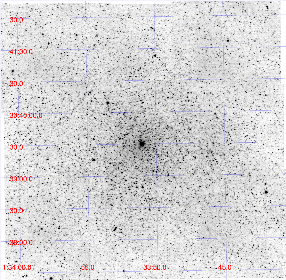
Figure 1: UFTI K-band mosaic of the central square kiloparsec of M 33.

The resulting UFTI K-band mosaic is shown in Fig. 1. The central $5^{\prime\prime}$ diameter region of the nuclear star cluster is unresolved. This is surrounded by a region of $\sim 1^{\prime}$ diameter with a considerably higher stellar density, the “bulge”. Outside that, the image is dominated by the inner part of the disc of M 33, although it is difficult to make out the spiral arm pattern that is a conspicuous feature of M 33 at larger distances from the nucleus.

3 Photometry

Photometry was obtained for all stars within each frame by automated fitting of a model of the Point Spread Function (PSF), using the daophot/allstar software suite (Stetson 1987). Depending on the conditions we used either a constant or quadratically-varying PSF. For the images with a constant-PSF model we selected 15–30 isolated PSF stars; for the other images we selected 50–100 PSF stars. The final PSF model was made from the frame from which all neighbours of the PSF stars had been subtracted. All PSF stars were selected based on their $\chi$ (goodness-of-fit) and “sharpness” value; ideally, $\chi=1$ and sharpness $=0$ for stars with realistic uncertainty estimates. The resulting PSF-subtracted image was then examined, rejecting any PSF stars that had not subtracted perfectly from the image.

The individual images were aligned using the daomaster routine, which computes the astrometric transformation equation coefficients from the daophot/allstar results. We combined the individual images using the montage2 routine (Stetson 1994), and then co-added these three J-, H- and K-band images with the imarith task in Iraf to create a master mosaic of the central $4^{\prime}\times 4^{\prime}$ of M 33. A master catalogue of stars was then created by application of daophot/allstar to this master mosaic, using over 100 PSF stars to create the (quadratically-varying) PSF model. We thus obtained photometry for 18,518 stars.

The master catalogue was used as input for allframe, which simultaneously performed PSF-fitting photometry on these stars within each of the individual images. The PSF created from the master mosaic did not fit perfectly to the stars in the individual images, mainly because of variations in the Full Width at Half Maximum (FWHM). Therefore, we used instead the PSFs created for each image separately.

Figure 2: The $\chi$ (top) and sharpness (bottom) values, vs. K-band magnitude for stars in one of the individual frames. The dashed line shows the selection limit on the $\chi$ value.

Figure 3: Average $\chi$ (top) and sharpness (bottom) values, vs. K-band magnitude, after applying a selection on $\chi$ (see text).

In Fig. 2 we show the $\chi$ and sharpness values vs. K-band magnitude for one of our individual frames. We removed non-stellar objects by setting limits on the $\chi$ value, per individual frame. We did not set limits on the sharpness value. Stars were selected with $\chi$ values below the dashed line in Fig. 2 (but this differs for other frames). For this frame, most stellar objects have $\chi<3$, but one can notice some bright objects with slightly larger $\chi$ values; this may be due to inaccuracies in the adopted PSF model. We also removed objects from the catalogue if they obeyed the $\chi$ criterion in only 10% of the measurements for that object. In this way our final catalogue has 18,398 stellar objects. The average $\chi$ and sharpness values of objects in the catalogue are shown in Fig. 3.

Aperture corrections to the PSF-fitting photometry were determined using the daogrow routine (Stetson 1990) to construct growth-curves for each frame from which all stars had been subtracted except the PSF stars. We then applied the collect routine (Stetson 1993) to calculate the ”aperture correction”, i.e. the difference between the PSF-fitting and large-aperture magnitude of these stars. We added this value to each of the PSF-fitting magnitudes.

Photometric calibration was then performed in a two-step manner. First, the standard star measurements were used to calibrate the frames on those nights. For the frames without standard star measurements we adopted the documented zero points (although this is not really needed). Airmass-dependent atmospheric extinction corrections were applied adopting the extinction coefficients derived by Krisciunas et al. (1987). In the second step, we calibrated the frames relative to one another. For this, we selected approximately 1000 stars in common between all frames belonging to a specific quadrant, within the magnitude interval $K\in[16...18]$, and averaged the magnitudes of these selected stars in each frame. The photometry was brought in line with each other by applying corrections between $-0.052$ to 0.067 mag (but usually much smaller). Checks on the overlap regions showed that no additional corrections had to be applied to the photometry between the four quadrants. Finally, the photometry was transformed onto the 2MASS system by using the tranformation equations derived by Carpenter et al. (2001).

3.1 Survey completeness

Figure 4: Completeness as a function of J- (dots, solid line), H- (squares, dotted) and K-band (crosses, dashed) magnitude.

To estimate the completeness of our catalogue and the effect of blending we added 300 artificial stars in each of 5 trials to the master mosaic using the daophot/addstar task (Stetson 1987). We added stars in 0.5-mag bins starting from $K=16$ mag until $K=20.5$ mag (until 21 mag in $H$ and 21.5 mag in $J$). Stars were positioned randomly in the image and Poisson noise was added. Then, we repeated the daofind/allstar/allframe procedure on the new frame as described before. Once the photometry was done and the final list created we used daomaster to evaluate what fraction of stars was recovered. As one can see in Fig. 4 our catalogue is essentially complete down to $K\sim 17$ mag, complete to $>88$% down to $K\sim 18$ mag (near the RGB tip, see below), dropping to below 50% at $K=19$ mag. The J-band reaches similar completeness levels but at about a magnitude fainter, and the H-band lies somewhere in between those two.

Figure 5: Difference between input magnitude and recovered magnitude (from a K-band image) vs. distance from the centre of M 33, for four values of the input magnitude. Stars observed near the edges of the frames are highlighted in red, and the dispersion is indicated in the form of an errorbar in each panel.

We also examined the accuracy of our photometry by adding artificial stars to one of the individual frames. Like before, we repeated the photometry for this frame after adding 300 stars in each of 5 trials, where the added stars were given magnitudes $K\in(16,17,18,19)$. The difference between input magnitude and recovered magnitude is small, $|\Delta K|<0.2$ mag, except very near the centre of M 33, $r<5^{\prime\prime}$, where it reaches $\Delta K<-1$ mag (Fig. 5), i.e. the recovered stars are brighter than the input stars. We attribute this to severe blending in the unresolved nucleus of M 33. The same pattern is seen for $K=17$ and 18 mag just with increased values for $\Delta K$. Stars that are located near the edges of the images are recovered with the same degree of flux conservation as stars elsewhere in the images, so we conclude that the photometry is accurate also for stars near the frame edges. At $K=19$ mag most of the recovered stars are brighter than the input stars irrespective of distance from the centre. By then, crowding has become substantial: the stellar density reaches $\sim 0.06$–0.11 star per square arcsec down to $K=19.5$ mag.

The scientific objectives of our project concentrate on the use of AGB stars and RSGs, that have $K<18.3$ mag, hence our analysis is not seriously compromised by the completeness limit and blending of stars except within the inner few arcseconds of M 33. It is also important to note that, while absolute photometry in crowded regions may be compromised, relative photometry between images can be more accurate, and variability throughout a series of measurements may be detected with confidence at a level – or below that – of the errors on individual measurements.

4 Variability analysis

Variable star candidates were identified with the newtrial routine (Stetson 1993) which uses the technique developped by Welch & Stetson (1993) and Stetson (1996). This method first calculates the $J$ index:

$$J=\frac{\Sigma_{k=1}^{n}w_{k}\ {\rm sign}(P_{k})\sqrt{|P_{k}|}}{\Sigma_{k=1}^{n}w_{k}}.$$ (1)

Here, observations $i$ and $j$ have been paired and each pair $k$ has been given a weight $w_{k}$; the product of the normalised residuals, $P_{k}=(\delta_{i}\delta_{j})_{k}$, where $\delta_{i}=(m_{i}-\langle m\rangle)/\epsilon_{i})$ is the deviation of measurement $i$ from the mean, normalised by the error on the measurement, $\epsilon_{i}$. Note that $\delta_{i}$ and $\delta_{j}$ may refer to measurements taken in different filters. The $J$ index has a large positive value for variable stars and tends to zero for data containing random noise only.

In circumstances where we are dealing with a small number of observations or corrupt data we gain from also calculating the Kurtosis index:

$$K=\frac{\frac{1}{N}\Sigma_{i=1}^{n}|\delta_{i}|}{\sqrt{\frac{1}{N}\Sigma_{i=1}^{N}\delta_{i}^{2}}}.$$ (2)

The value of $K$ depends on the shape of the light-curve: $K=0.9$ for a sinusoidal light variation, where the source spends most time near the extrema, $K=0.798$ for a Gaussian distribution, which is concentrated towards the average brightness level (as would random noise), and $K\rightarrow 0$ for data affected by a single outlier (when $N\rightarrow\infty$).

The variability index that we calculate in this paper depends on both the $J$ and $K$ indices and is defined by (Stetson 1996):

$$L=\frac{J\times K}{0.798}.$$ (3)

Figure 6: Histogram of variability index for two ways of pairing three measurements $a$, $b$ and $c$: (dashed:) $ab$, $bc$; (solid:) $ab$, $bc$, $ac$. The latter is the extended method proposed by Stetson (1996) and which is adopted here.

Measurements can be paired if they are taken close in time compared to the (expected) period of variability – which for the type of stars we search for within the context of this programme is of order 100 days or longer. If within a pair of observations only one measurement is available for a particular star then the weight of the pair for that star is set to 0.5. Stetson (1996) extended this principle to involve more than two measurements at a time: three measurements $a$, $b$ and $c$ taken within a time-span less than the shortest period can be paired as $ab$, $bc$, and $ac$ rather than just $ab$ and $bc$. There is no discernable difference in the variability index for different pairing schemes (Fig. 6), and we decided to use Stetson’s extended method of pairing here.

Figure 7: Variability index $L$ vs. K-band magnitude. The dashed line indicates our threshold for identifying variable stars, at $L>4$.

Figure 8: Histograms of the variability index $L$, for several K-band magnitude bins. The solid lines show Gaussian functions fitted to the histograms.

Fig. 7 shows the variability index $L$ vs. K-band magnitude, where the dashed line indicates our threshold for detected variability: $L>4$. There is a remarkable “branch” of variable stars between $K\sim 16$–18 mag which are likely AGB stars that show Mira-type variability, with hardly any fainter variables and a modest number of brighter variables. Histograms of the variability index for several K-band magnitude intervals in the range 16–18.5 mag are shown in Fig. 8. To determine the optimal variability threshold, a Gaussian function was fitted to each of these histograms. While the Gaussian function is a near-perfect fit to the symmetrical distributions at low values for $L$, the distributions show a pronounced tail towards higher values for $L$. The departure from the Gaussian shape occurs typically around $L\approx 4$.

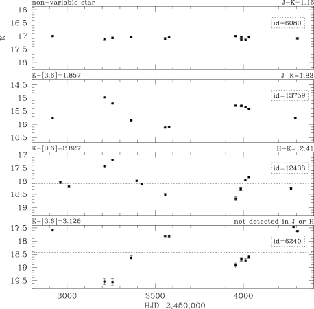
Figure 9: Example light-curves of three very red variable stars with large amplitude and probably long period (around 700 days), with a non-variable star in the top panel for comparison.

We thus identified 812 variable stars in the central square kiloparsec of M 33. (A further 6 were rejected on the basis of their large $\chi$ values.). Three examples of large-amplitude, likely long-period variability are shown in Fig. 9, with a non-variable star for comparison. These variable stars have a period around 700 days and much redder colours than the bulk of the non-variable stars.

4.1 Amplitudes of variability

A measure for the ampltidue of variability can be obtained by assuming a sinusoidal light-curve shape. The standard deviation of the unit sine function is 0.701. Hence, for a standard deviation in our data, $\sigma$, the amplitude estimate would be $A=2\times\sigma/0.701$.

Figure 10: Standard deviation vs. number of measurements that randomly sample a unit sine curve.

In practice, however, for small sets of data the standard deviation depends on the number of measurements. Fig. 10 shows the result of simulations: it is clear that when only a handful of measurements are available, the standard deviation that is calculated will, on average, drop below the asymptotic value (0.701 for the sine function) that is reached for well-sampled light-curves, as well as becoming less reliable. We set $N=6$ as a minimum for applying our method to estimate the amplitude from the standard deviation. From Fig. 10 one can see that, by then, the standard deviation will have converged to within 10% of the asymptotic value.

Figure 11: Estimated amplitude, $A_{\rm K}$, of variability vs. K-band magnitude. Crosses indicate variables with $A_{\rm K}>2$ mag but with only six or fewer measurements.

The estimated K-band amplitude of variability is plotted vs. K-band magnitude in Fig. 11. Variability could have been detected for $A_{\rm K}>0.2$ mag. There is a clear tendency for the amplitude to diminish with increasing brightness, which is a known (Wood et al. 1992; Wood 1998; Whitelock et al. 2003) and to some extent understood (van Loon et al. 2008) trend. Among the variables with $A_{\rm K}>2$ mag, four have six or fewer measurements and their amplitudes are therefore unreliable – these are highlighted in Fig. 11 with crosses, and includes the one with the highest estimate for the amplitude. Disregarding those, the amplitudes stay below $A_{\rm K}\sim 3$ mag and generally $A_{\rm K}<2$ mag. Very dusty AGB stars are known to reach such large amplitudes (Wood et al. 1992; Wood 1998; Whitelock et al. 2003), but they are very rare. Light-curves of a few large-amplitude variables in our survey were displayed in Fig. 9.

Figure 12: Estimated amplitude, $A_{\rm K}$, of variability vs. colour. Crosses indicate variables with $A_{\rm K}>2$ mag but with only six or fewer measurements (two further such stars have no J- or H-band detection).

The estimated K-band amplitude of variability is plotted vs. the $J-K$ and $H-K$ colour in Fig. 12. There is a clear sequence branching off the bulk of stars towards redder colours and associated larger amplitudes (cf. Fig. 9). This is not surprising as large-amplitude variability is known to be associated with profuse dust formation (Wood et al. 1992; Wood 1998; Whitelock et al. 2003), and the less-luminous larger-amplitude stars will be rendered obscured much more readily than their more luminous siblings (van Loon et al. 1997).

A small number of very large amplitude stars form a vertical sequence around $J-K\sim 1$ and $H-K\sim 0$ mag (Fig. 12), but these are suspect. We inspected all of the stars with $A_{\rm K}>1.7$ mag by eye, and found that they fall into either of two categories: (1) nine bright stars, $15.3<K<18$ mag, that are affected by blending. In some frames these were mistaken for another faint star, resulting in a spuriously large amplitude. The small number of variable stars that are affected by such complications ($\sim 1$% ) indicates that these are rare incidences; (2) nine faint stars, $K>18$ mag, which were not visibly affected by blending. Two of these in actual fact do have red colours, $J-K=2.3$ mag ($A_{\rm K}=1.9$ mag) and $J-K=2.5$ mag ($A_{\rm K}=2.0$ mag), and they may be dusty large-amplitude variables. The same could explain the non-detection in the J- and H-band of four other stars in this category. That leaves three stars that appear blue for their large amplitude. These are located near the edge of the frame, resulting in particularly poor photometry on one or two occasions. Again, these respresent very few occurrences of such effects.

5 Description of the catalogue

Table 3: Description of the photometric catalogue.

Column No.	Descriptor
Part I: stellar mean properties (18,398 lines)
1	Star number
2	Right Ascension (J2000)
3	Declination (J2000)
4	Mean J-band magnitude
5	Error in $\langle J\rangle$
6	Mean H-band magnitude
7	Error in $\langle H\rangle$
8	Mean K-band magnitude
9	Error in $\langle K\rangle$
10	Number of J-band measurements
11	Number of H-band measurements
12	Number of K-band measurements
13	Mean $\chi$ value from daophot
14	Mean sharpness value from daophot
15	Variability index $J$
16	Kurtosis index $K$
17	Variability index $L$
18	Estimated K-band amplitude
Part II: multi-epoch data (356,303 lines)
1	Star number
2	Epoch (HJD–2,450,000)
3	Filter (J, H or K)
4	Magnitude
5	Error in magnitude
6	$\chi$ value from daophot
7	Sharpness value from daophot

The photometric catalogue including all variable and non-variable stars is made publicly available at the Centre de Données astronomiques de Strasbourg (CDS). The content is described in Table 3. It is composed of two parts, part I comprising the mean properties of the stars and part II tabulating all the photometry (for the benefit of generating lightcurves, for instance).

The astrometric accuracy of the catalogue is $\approx 0.2^{\prime\prime}$ r.m.s., tied to the 2MASS system. This accuracy was found to be consistent with the results from our cross-correlations with three other optical and IR catalogues (cf. Section 6.2).

6 Discussion

6.1 The near-IR variable star population

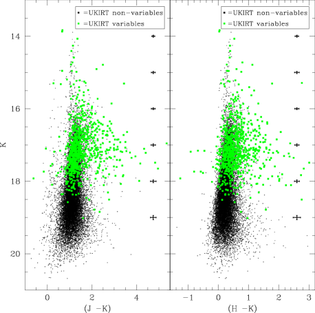
Figure 13: Near-IR colour–magnitude diagrams showing the UKIRT variable stars in green. Average errorbars are plotted for 1-mag intervals in the K-band.

Fig. 13 presents near-IR colour–magnitude diagrams for our field in M 33, with highlighted in green the variable stars we identified. Large-amplitude variable stars are mainly found between $K\sim 16$–18 mag, and are conspicuously absent among fainter stars. Some very bright variable stars are found, too. Striking is the predominance of variable stars among the redder stars that lie to the right of the vertical sequence of the bulk of the stars.

Figure 14: Distribution of all UKIRT sources (solid) and UKIRT variable stars (dotted), as a function of near-IR brightness.

Figure 15: Distribution of all UKIRT sources with $K<19$ mag (solid) and UKIRT variable stars (dotted), as a function of near-IR colour.

Better quantified, albeit degenerate, are histograms of the distributions over brightness (Fig. 14) and colour (Fig. 15). Between $K\sim 16$–17 mag, and likewise for $(H-K)>0.7$ mag, the number of variable stars per histogram bin reaches the same value as the number of all UKIRT sources per bin – note, however, that the bins in the former sample a three times larger range in brightness or colour, so the true fraction of variables among those stars is closer to a third. Still, at $(J-K)>2$ mag or $(H-K)>1$ mag (and with $K<19$ mag) almost all stars are variable.

Between $K\sim 17$–18 mag the fraction of variable stars drops to only a few per cent; the frequency of stars increases but the frequency of variable stars decreases. This is due mainly to a combination of two factors. Firstly, lower on the AGB there is a greater contribution from stars that will still evolve to higher luminosity and lower temperature (thus exacerbating the brightness increase in the K-band) before they develop large-amplitude variability. That is precisely the reason why our project aims to use the variable stars as tracers of the distribution of stars over birth-mass. Secondly, the relation between birth-mass and K-band brightness flattens dramatically for low-mass (relatively faint) AGB stars. This is explored in much more detail in Paper II.

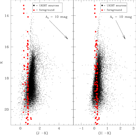
Figure 16: Estimated contamination by foreground stars (in red), from a simulation with trilegal (Girardi et al. 2005).

To assess the level of contamination by foreground stars, we performed a simulation with the trilegal tool (Girardi et al. 2005). Adopting default parameters for the structure of the Galaxy, in a 0.005 deg² field in the direction ($l=133.61^{\circ}$, $b=-31.33^{\circ}$) only a small number of foreground stars are expected (Fig. 16). These do not generally cause significant problems – they all have fairly neutral colours – except that very bright stars at $K<14$ mag are likely to be foreground stars and not stars within M 33. Also indicated in Fig. 16 are the reddening vectors equivalent to a visual extinction of $A_{\rm V}=10$ mag, adopting extinction coefficients of $A_{\rm K}=0.12A_{\rm V}$, $A_{\rm H}=1.6A_{\rm K}$ and $A_{\rm J}=2.6A_{\rm K}$ (cf. Becklin et al. 1978; Savage & Mathis 1979; Rieke, Rieke & Paul 1989).

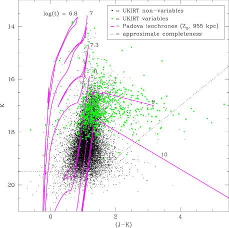
Figure 17: Colour–magnitude diagram of $(J-K)$, with UKIRT variable stars highlighted in green. Overplotted are isochrones from Marigo et al. (2008) for solar metallicity and a distance modulus of 24.9 mag.

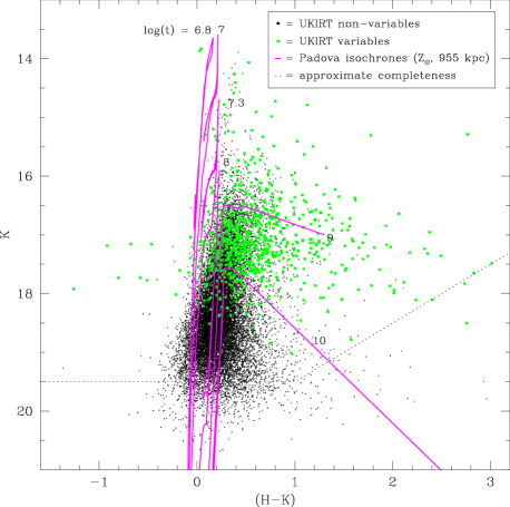
Figure 18: Colour–magnitude diagram of $(H-K)$, with UKIRT variable stars highlighted in green. Overplotted are isochrones from Marigo et al. (2008) for solar metallicity and a distance modulus of $\mu=24.9$ mag.

We characterise the stellar population in the central regions of M 33 further by confrontation of the colour–magnitude diagrams with isochrones calculated by Marigo et al. (2008) (Figs. 17 and 18). The isochrones were calculated for solar metallicity, which is appropriate for the central disc population in M 33 (cf. Magrini et al. 2007; Rosolowsky & Simon 2008); a check was made for a metallicity half that of the Sun and no appreciable difference was found in the red (super-)giant branches. The adopted distance modulus of $\mu=24.9$ mag appears to be appropriate as it fits well with the magnitude at which the variable stars become abundant and the K-band luminosity function shows a break in the slope (Fig. 14), at the location of the RGB tip, as well as to the maximum extent in luminosity of the RSGs. Indeed, RSGs are found all the way until the earliest age (highest birth mass) at which they are expected, $t\approx 10$ Myr.

The isochrones of Marigo et al. (2008) are the most realistic models easily available for comparison with dust-producing stellar populations, as they include predictions for the onset of large-amplitude pulsation, the associated mass-loss rate and dust-formation rate, and the resulting changes in the spectral energy distribution (SED) as the dust redistributes optical light over the IR domain. This causes the drastic excursions of the isochrones towards red colours as soon as the dust envelope becomes optically thick at near-IR wavelengths; hence it is accompanied by a drop in K-band brightness as the peak of the SED shift towards (even) longer wavelengths. The 1-Gyr isochrones show consistency with the red branch of UKIRT variables. The 10-Gyr isochrones seem to show a rather too rapid decline in the K band compared to observations, but this may be due to the fact that these stars experience very large reddening and thus become readily undetectable – this is corroborated by the isochrones as well as by empirical evidence of low-mass AGB stars becoming obscured by circumstellar dust much more readily than their more massive siblings (van Loon et al. 1997).

6.2 Cross-identifications in other catalogues

We cross-correlate our UKIRT variability search results with those from two intensive optical monitoring campaigns (CFHT, Hartman et al. 2006; DIRECT, Macri et al. 2001) and the mid-IR variability search performed with the Spitzer Space Telescope (McQuinn et al. 2007). We also compare with the optical catalogue of Rowe et al. (2005) which includes narrow-band filters that they used to identify carbon stars. The matches were obtained by search iterations using growing search radii, in steps of $0.1^{\prime\prime}$ out to $1^{\prime\prime}$, on a first-encountered first-associated basis after ordering the principal photometry in order of diminishing brightness (K-band for the UKIRT catalogue, i-band/I-band for the optical catalogues, and 3.6-$\mu$m band for the Spitzer catalogue).

6.2.1 CFHT optical variability survey

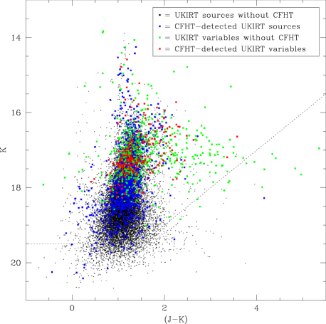
Figure 19: Near-IR colour–magnitude diagram showing the stars from the UKIRT survey that were and were not identified as variable stars in the CFHT optical variability survey (Hartman et al. 2006).

The Canada France Hawai’i Telescope (CFHT) optical variability survey (Hartman et al. 2006) was performed during 27 nights (comprising 36 individual measurements) between August 2003 and January 2005. The catalogue contains variable stars only, with photometry in the Sloan g^′-, r^′- and i^′-bands to a depth of approximately $i^{\prime}\approx 24$ mag. Out of 2 million point sources in a square-degree field, they identified $>1300$ candidate variable blue and red supergiants, $>2000$ Cepheids and $>19,000$ AGB and RGB LPVs.

Within the coverage of our UIST observations are located $\approx 1737$ variable stars from the CFHT catalogue. Out of these, 1481 (85%) were detected in our UKIRT survey, of which 247 were found by us to be variable. The CFHT variables that we did not identify as being variable are generally fainter than the RGB tip (Fig. 19) and thus not the LPVs we aimed to find for the purpose of our project, but they also include bright AGB stars and RSGs whose modest amplitudes (especially at IR wavelengths) may have led them to escape from our UKIRT variability search. Clearly, the dusty (reddened) AGB variables detected in our UKIRT survey were generally not detected in the CFHT survey.

6.2.2 DIRECT optical variability survey

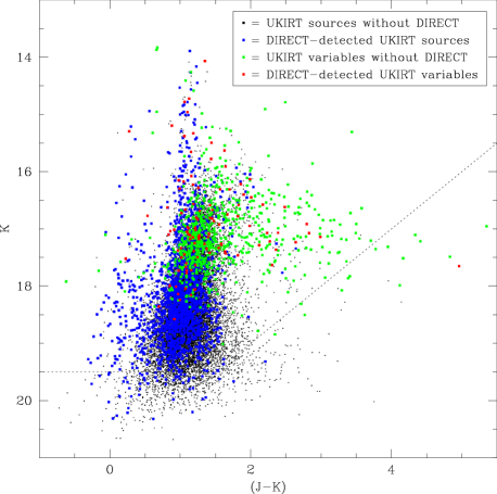
Figure 20: Near-IR colour–magnitude diagram showing the stars from the UKIRT survey that were and were not detected in the DIRECT optical variability survey (Macri et al. 2001).

The DIRECT optical variability survey (Macri et al. 2001) aimed to determine direct distances to M 31 and M 33 using detached eclipsing binaries and Cepheid variables. The catalogue is based on observations performed between September 1996 and October 1997, during 95 nights on the F. L. Whipple Observatory 1.2-m telescope and 36 nights on the Michigan–Dartmouth–MIT 1.3-m telescope. The catalogue contains Johnson B- and V-, and Cousins I-band photometry for all stars with $14.4<V<23.6$ mag, and lists the V-band $J$ variability index (cf. Section 4).

Within the coverage of our UIST observations are located $\approx 2644$ stars from the DIRECT catalogue (among which 113 have $J>0.75$, which the DIRECT survey team considered as the threshold for variability). Out of these, 2018 (76%) were detected in our UKIRT survey, of which 106 were found by us to be variable. Remarkably, most of the UKIRT variables (87%) were missed by the DIRECT survey (Fig. 20). This is due in part because the dusty variables are very faint in the optical, but surprisingly most of the not-so-dusty AGB variables are also missing from the DIRECT survey. The DIRECT survey seems to have been less successful in finding LPVs than the CFHT survey.

6.2.3 Carbon star survey

Rowe et al. (2005) used the CFHT and a four-filter system in 1999 and 2000 to cover most of M 33 including the central region. The filter system was designed to identify carbon stars on the basis of their cyanide (CN) absorption as opposed to other red giants that display titanium-oxide (TiO) absorption, using narrow-band filters centred on 8120 and 7777 Å, respectively. They added broad-band Mould V- and I-band filters to aid in selecting cool stars. Carbon stars in their scheme have [CN]$-$[TiO] $>0.3$ and $V-I>1.8$ mag, and M-type stars have [CN]$-$[TiO] $<-0.2$ mag at the same V–I criterion (they only considered stars for this purpose that had errors on these colours of $<0.05$ mag).

The region covered by our UKIRT survey contains $\sim$100,000 stars from the Rowe et al. catalogue; all but 837 of our objects were identified among these. The problem with such density of optical sources is that chance co-incidences are common. When a pre-selection is made of stars that are probably carbon stars or M-type stars, which are likely to have been detected at near-IR wavelengths, then the number of stars to correlate with is drastically reduced. The average offsets between these and their identified UKIRT counterparts are only $0.02^{\prime\prime}$ in both RA and Dec.

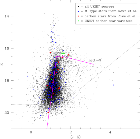
Figure 21: Near-IR colour–magnitude diagram showing the M-type and carbon stars from the Rowe et al. (2005) survey that were detected in our UKIRT survey. A 1-Gyr isochrone from Marigo et al. (2008) is shown for comparison.

The M-type stars follow the main giant branch (Fig. 21), avoiding the blue edge which is expected to be occupied by K-type giants without strong molecular absorption. The carbon stars are consistent with ages of $t\sim 1$ Gyr or a little younger, i.e. birth masses around 2–3 M_⊙. Two of the three carbon stars that are identified as UKIRT variables show signs of reddening presumably due to circumstellar dust; these are also among the brightest carbon stars and thus represent the termination point in their evolution. The faintest carbon stars are fainter than the tip of the RGB; while unexpected for carbon stars formed by thermal pulses on the AGB, faint carbon stars are known in other, generally metal-poor, populations, e.g., in the Sagittarius dwarf iregular galaxy (Gullieuszik et al. 2007) or in the Galactic globular cluster $\omega$ Centauri (van Loon et al. 2007).

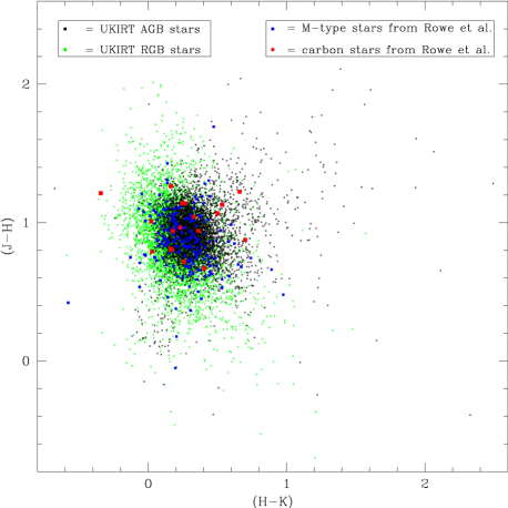
Figure 22: Near-IR colour–colour diagram showing the M-type and carbon stars from the Rowe et al. (2005) survey that were detected in our UKIRT survey. Stars with $18<K<19.5$ mag and errors on the colours $<0.25$ mag are labelled as RGB stars, whilst stars with $16<K<18$ mag and errors on the colours $<0.25$ mag are labelled as AGB stars

A colour-colour representation is shown in Fig. 22, where a crude distinction is made between RGB and AGB stars. Again, the reddened stars are AGB stars; RGB stars displaying a red J–K colour usually do not display a red H–K colour (or vice versa), suggesting that they are not (much) affected by reddening but that photometric uncertainties become larger. The M-type and carbon stars from Rowe et al. (2005) are generally constrained to the AGB, with a few carbon stars showing signs of reddening.

Though not many stars in Rowe et al. have errors on their colours of $<0.05$ mag, and the suspicion is that many more of the UKIRT sources are carbon stars or M-type stars, carbon stars do not seem to dominate the stellar population in the central square kpc of M 33. This onfirms the trend of the ratio of carbon to M-type stars found by Rowe et al. (2005) to drop from typically $\approx 0.5$ to $<0.2$ in the central few arcminutes, and it is corroborating evidence for a predominantly solar-metallicity population as carbon stars are more common among populations with sub-solar metallicity (Groenewegen 1999).

6.2.4 Spitzer mid-IR variability survey

McQuinn et al. (2007) used five epochs of Spitzer Space Telescope observations of M 33 obtained in the 3.6-, 4.5- and 8-$\mu$m bands, to identify variable stars in a manner which is broadly similar to our approach with UKIRT.

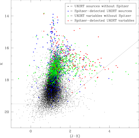
Figure 23: Near-IR colour–magnitude diagram showing the stars from the UKIRT survey that were and were not detected in the Spitzer variability survey (McQuinn et al. 2007).

In the central regions of M 33, crowding and strong, complex diffuse emission severely limited the capability of the Spitzer survey. It yielded 784 sources in roughly the same area covered by our UIST data. Among these, 557 are in our photometric catalogue, most of them are brighter than the RGB tip. Of the 227 Spitzer sources that we did not recover, 13 had been rejected from our catalogue because of too high $\chi$ values – these were at the edges of frames and only covered in part. Hence the recovery rate is well above 70%. The success rate of the Spitzer survey in detecting stars from our UKIRT survey is particularly good for the RSGs, the brightest AGB stars, and the dusty AGB variables (Fig. 23); AGB stars not in the Spitzer catalogue are generally situated closer to the centre of M 33 where crowding increases. Indeed, blending is quite common, with the Spitzer source being centred in between the position of two similarly-bright stars.

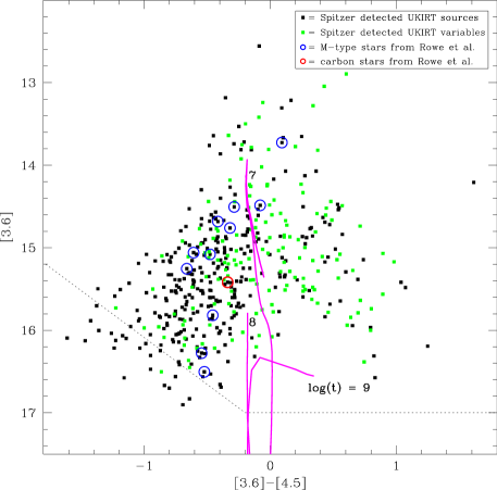
Figure 24: Mid-IR colour–magnitude diagram from Spitzer photometry of UKIRT sources, with UKIRT variables highlighted in green and M-type and carbon stars from Rowe et al. (2005) circled in blue and red, respectively. Isochrones from Marigo et al. (2008) for 10 Myr, 100 Myr and 1 Gyr are drawn. The dotted line indicates the approximate detection limit of the Spitzer survey.

The mid-IR colour–magnitude diagram (Fig. 24) shows a well-populated, skewed sequence off from which a branch extends towards redder colour and fainter 3.6-$\mu$m brightness. The latter is comprised of dust-enshrouded objects, among which a relatively greater proportion are UKIRT variables. UKIRT variables are also abound among the brightest 3.6-$\mu$m sources in the diagram; these are massive AGB stars and RSGs. The confirmed M-type stars form a sequence of increasing 3.6-$\mu$m brightness, and the only confirmed carbon star that is detected by Spitzer (and us) sits roughly half-way and marginally to the red of that sequence. None of these are on the red branch of dust-enshrouded objects, probably because the optical photometry was not deep enough for them to have been detected or not accurate enough for them to have been classified.

The isochrones confirm the picture just outlined in a qualitative manner, but there is a surprisingly large discrepancy between the Spitzer photometry and the isochrones. The Spitzer photometry appears too blue at faint magnitudes, by at least several tenths of a magnitude – we consider it unlikely that the colours are really as negative as $([3.6]-[4.5])\approx-0.7$ mag (a factor two depression of the 4.5-$\mu$m brightness). For the isochrones to match the 3.6-$\mu$m brightness, in agreement with the way in which they match (well) the near-IR colour–magnitude diagrams, the isochrones would need to be shifted to higher 3.6-$\mu$m brightness levels by at least a magnitude or the data need to be diminished by that amount. We find either solution unsatisfactory, and suspect that both the Spitzer photometry and isochrones may need adjustments. We postpone a thorough investigation to Paper III in which we model the SEDs.

7 Conclusions

UKIRT was used to monitor the central $4^{\prime}\times 4^{\prime}$ (square kpc) of Local Group spiral galaxy M 33 (Triangulum) in the K-band filter with additional observations in the J- and H-band filters.

As a result, a photometric catalogue was compiled of 18,398 stars among which 812 were identified as exhibiting large-amplitude variability. Inspection of the lightcurves and locations on the colour–magnitude diagram with respect to theoretical models of stellar evolution leads us to conclude that most of these variable stars are AGB stars or RSGs, and that most of the very dusty stars – that are heavily reddened even at IR wavelengths – are variable.

Our catalogue is cross-correlated with previous optical monitoring surveys, an optical carbon star survey, and the Spitzer mid-IR survey. The UKIRT catalogue is vastly more complete for the dusty variables than the optical surveys, but also much more complete than the Spitzer survey. Our catalogue is made public at CDS.

In the next papers in this series, our catalogue will be used to describe the star formation history and the dust production in the central regions of M 33.

References

- [Becklin et al.(1978)] Becklin E. E., Neugebauer G., Willner S. P., Matthews K., 1978, ApJ, 220, 831
- [Bonanos et al.(2006)] Bonanos A. Z. et al., 2006, ApJ, 652, 313
- [Bowen (1988)] Bowen G. H., 1988, ApJ, 329, 299
- [Bowen & Willson (1991)] Bowen G. H., Willson L. A., 1991, ApJ, 375, L53
- [Carpenter (2001)] Carpenter J. M., 2001, AJ, 121, 2851
- [Freedman, Wilson & Madore (1991)] Freedman W. L., Wilson C. D., Madore B. F., 1991, ApJ, 372, 455
- [Galleti, Bellazzini & Ferraro (2004)] Galleti S., Bellazzini M., Ferraro F. R., 2004, A&A, 423, 925
- [Girardi et al.(2005)] Girardi L., Groenewegen M. A. T., Hatziminaoglou E., da Costa L., 2005, A&A, 436, 895
- [Groenewegen (1999)] Groenewegen M. A. T., in: Asymptotic Giant Branch Stars, eds. T. Le Bertre, A. Lèbre and C. Waelkens, IAU Symposium 191, p535
- [Gullieuszik et al.(2007)] Gullieuszik M., Rejkuba M., Cioni M. R., Habing H. J., Held E. V., 2007, A&A, 475, 467
- [Hartman et al.(2006)] Hartman J. D., Bersier D., Stanek K. Z., Beaulieu J.-P., Kałuny J., Marquette J.-B., Stetson P. B., Schwarzenberg-Czerny A., 2006, MNRAS, 371, 1405
- [Kim et al.(2002)] Kim M., Kim E., Lee M. G., Sarajedini A., Geisler D., 2002, AJ, 123, 244
- [Krisciunas et al.(1987)] Krisciunas K. et al., 1987, PASP, 99, 887
- [Macri et al.(2001)] Macri L. M., Stanek K. Z., Sasselov D. D., Krockenberger M., Kałuny J., 2001, AJ, 121, 861
- [Levesque (2010)] Levesque E. M., 2010, in: Hot and Cool – Bridging Gaps in Massive Star Evolution, eds. C. Leitherer, P. Bennett, P. Morris and J. Th. van Loon, ASPC (San Francisco: ASP), 425, p103
- [Levesque et al.(2005)] Levesque E. M., Massey P., Olsen K. A. G., Plez B., Josselin E., Maeder A., Meynet G., 2005, ApJ, 628, 973
- [Magrini et al.(2007)] Magrini L., Vílchez J. M., Mampaso A., Corradi R. L. M., Leisy P., 2007, A&A, 470, 865
- [Marigo et al.(2008)] Marigo P., Girardi L., Bressan A., Groenewegen M. A. T., Silva L., Granato G. L., 2008, A&A, 482, 883
- [McConnachie et al.(2004)] McConnachie A. W., Irwin M. J., Ferguson A. M. N., Ibata R. A., Lewis G. F., Tanvir N., 2004, MNRAS, 350, 243
- [McQuinn et al.(2007)] McQuinn K. B. W. et al., 2007, ApJ, 664, 850
- [Mochejska et al.(2001a)] Mochejska B. J., Kałuny J., Stanek K. Z., Sasselov D. D., Szentgyorgyi A. H., 2001a, AJ, 121, 2032
- [Mochejska et al.(2001b)] Mochejska B. J., Kałuny J., Stanek K. Z., Sasselov D. D., Szentgyorgyi A. H., 2001b, AJ, 122, 2477
- [Pierce, Jurcevi&́ Crabtree (2000)] Pierce M. J., Jurcević J. S., Crabtree D., 2000, MNRAS, 313, 271
- [Rieke, Rieke & Paul (1989)] Rieke G. H., Rieke M. J., Paul A. E., 1989, ApJ, 336, 752
- [Rizzi et al.(2007)] Rizzi L., Tully R. B., Makarov D., Makarova L., Dolphin A. E., Sakai S., Shaya E. J., 2007, ApJ, 661, 815
- [Rosolowsky & Simon (2008)] Rosolowsky E., Simon J. D., 2008, ApJ, 675, 1213
- [Rowe et al.(2005)] Rowe J. F., Richer H. B., Brewer J. P., Crabtree D. R., 2005, AJ, 129, 729
- [Sarajedini et al.(2000)] Sarajedini A., Geisler D., Schommer R., Harding P., 2000, AJ, 120, 2437
- [Sarajedini et al.(2006)] Sarajedini A., Barker M. K., Geisler D., Harding P., Schommer R., 2006, AJ, 132, 1361
- [Savage & Mathis (1979)] Savage B. D., Mathis J. S., 1979, ARA&A, 17, 73
- [Scowcroft et al.(2009)] Scowcroft V., Bersier D., Moul J. R., Wood P. R., 2009, MNRAS, 396, 1287
- [Stetson (1987)] Stetson P. B., 1987, PASP, 99, 191
- [Stetson (1990)] Stetson P. B., 1990, PASP, 102, 932
- [Stetson (1993)] Stetson P. B., 1993, in: Stellar Photometry – Current Techniques and Future Developments, eds. C. J. Butler and I. Elliott, IAU Coll. Ser. 136 (Cambridge: Cambridge University Press), p291
- [Stetson (1994)] Stetson P. B., 1994, PASP, 106, 250
- [Stetson (1996)] Stetson P. B., 1996, PASP, 108, 851
- [Tiede, Sarajedini & Barker (2004)] Tiede G. P., Sarajedini A., Barker M. K., 2004, AJ, 128, 224
- [U et al.(2009)] U V., Urbaneja M. A., Kudritzki R.-P., Jacobs B. A., Bresolin F., Przybilla N., 2009, ApJ, 704, 1120
- [van Loon (2010)] van Loon J. Th., 2010, in: Hot and Cool – Bridging Gaps in Massive Star Evolution, eds. C. Leitherer, P. Bennett, P. Morris and J. Th. van Loon, ASPC (San Francisco: ASP), 425, p279
- [van Loon et al.(1997)] van Loon J. Th., Zijlstra A. A., Whitelock P. A., Waters L. B. F. M., Loup C., Trams N. R., 1997, A&A, 325, 585
- [van Loon et al.(1999)] van Loon J. Th., Groenewegen M. A. T., de Koter A., Trams N. R., Waters L. B. F. M., Zijlstra A. A., Whitelock P. A., Loup C., 1999, A&A, 351, 559
- [van Loon et al.(2005)] van Loon J. Th., Cioni M.-R. L., Zijlstra A. A., Loup C., 2005, A&A, 438, 273
- [van Loon et al.(2007)] van Loon J. Th., van Leeuwen F., Smalley B., Smith A. W., Lyons N. A., McDonald I., Boyer M. L., 2007, MNRAS, 382, 1353
- [van Loon et al.(2008)] van Loon J. Th., Cohen M., Oliveira J. M., Matsuura M., McDonald I., Sloan G. C., Wood P. R., Zijlstra A. A., 2008, A&A, 487, 1055
- [Vassiliadis & Wood (1993)] Vassiliadis E., Wood P. R., 1993, ApJ, 413, 641
- [Whitelock et al.(2003)] Whitelock P. A., Feast M. W., van Loon J. Th., Zijlstra A. A., 2003, MNRAS, 342, 86
- [Wood (1998)] Wood P. R., 1998, A&A, 338, 592
- [Wood (1999)] Wood P. R., in: Asymptotic Giant Branch Stars, eds. T. Le Bertre, A. Lèbre and C. Waelkens, IAU Symposium 191, p151
- [Wood et al.(1992)] Wood P. R., Whiteoak J. B., Hughes S. M. G., Bessell M. S., Gardner F. F., Hyland A. R., 1992, ApJ, 397, 552