The soft X-ray and narrow-line emission of Mrk 573 on kiloparcec scales

Abstract

We present a study of the circumnuclear region of the nearby Seyfert galaxy Mrk 573 using Chandra, XMM-Newton and Hubble Space Telescope (HST) data. We have studied the morphology of the soft ($\sf{<2~{}keV}$) X-rays comparing it with the [O III] and H$\rm{\alpha}$ HST images. The soft X-ray emission is resolved into a complex extended region. The X-ray morphology shows a biconical region extending up to 12 arcsecs (4 kpc) in projection from the nucleus. A strong correlation between the X-rays and the highly ionized gas seen in the [O III]$\mathrm{\lambda 5007}$ Å image is reported. Moreover, we have studied the line intensities detected with the XMM–Newton Reflection Grating Spectrometer (RGS) and used them to fit the low resolution EPIC/XMM–Newton and ACIS/Chandra spectra. The RGS/XMM–Newton spectrum is dominated by emission lines of C VI, O VII, O VIII, Fe XVII, and Ne IX, among others highly ionized species. A good fit is obtained using these emission lines found in the RGS/XMM–Newton spectrum as a template for Chandra spectra of the nucleus and extended emission, coincident with the cone-like structures seen in the [O III]/H$\rm{\alpha}$ map. The photoionization model Cloudy provides a reasonable fit for both the nuclear region and the cone-like structures showing that the dominant excitation mechanism is photoionization. For the nucleus the emission is modelled using two phases: a high ionization [log(U)=1.23] and a low ionization [log(U)=0.13]. For the high ionization phase the transmitted and reflected component are in a ratio 1:2, whereas for the low ionization the reflected component dominates. For the extended emission, we successfully reproduced the emission with two phases. The first phase shows a higher ionization parameter for the NW (log(U)=0.9) than for the SE cone (log(U)=0.3). Moreover, this phase is transmission dominated for the SE cone and reflection dominated for the NW cone. The second phase shows a low ionization parameter (log(U)=-3) and is rather uniform for NW and SEcones and equally distributed in reflection and transmission components. In addition, we have also derived the optical/infrared spectral energy distribution (SED) of the nucleus from high spatial resolution images of Mrk 573. The nuclear optical/infrared SED of the nucleus has been modeled by a clumpy torus model. The torus bolometric luminosity agrees very well with the AGN luminosity inferred from the observed hard X-ray spectrum. The optical depth along the line of sight expected from the torus modeling indicates a high neutral hydrogen column density in agreement with the classification of the nucleus of Mrk 573 as a Compton-thick AGN.

1. Introduction

Visible signatures of the direct interaction between the active galactic nuclei (AGN) and their host galaxies include kpc-scale [O III]- and H$\sf{\alpha}$-emitting regions, the so-called extended narrow-line region (ENLR), which is observed in many nearby Seyfert galaxies (Schmitt et al., 2003; Veilleux et al., 2003; Whittle & Wilson, 2004; Ramos Almeida et al., 2006). Understanding the AGN-host galaxy interaction and feedback is crucial for the study of both galaxy and AGN evolution (Silk & Rees, 1998; Kauffmann et al., 2003; Hopkins et al., 2006; Schawinski et al., 2007, 2009).

One of the most promising ways to study these interactions is through soft X-rays (Crenshaw et al., 1999, 2003; Dai et al., 2008). In the unified picture of AGN (Antonucci, 1993) the soft X-ray spectra of Type-2 Seyfert galaxies are expected to be affected by emission and scattering from the medium, which is also strongly influenced by the nuclear continuum. However, soft X-rays can also be produced through mechanical heating, as in shocks driven by supernova explosions in nuclear star-forming regions. Indeed, it is quite plausible that both effects are important (e.g. Mrk 3; Sako et al. 2000). This soft X-ray emission provides the opportunity to obtain an X-ray diagnostic for the physical properties of the interacting interstellar medium [ISM] (Young et al., 2001; Yang et al., 2001; Ogle et al., 2000, 2003; Bianchi et al., 2006; Evans et al., 2006; Kraemer et al., 2008).

The galaxy Mrk 573 has been extensively studied by many authors. Its active nucleus is hosted in an (R)SAB(rs)0+ galaxy. Mrk 573 is well-known for its extended, richly structured circumnuclear emission-line regions (Tsvetanov & Walsh, 1992). It has long been known to show a biconical structure and bright arcs and knots of line-emitting gas (Ferruit et al, 1999; Quillen et al., 1999) that are strongly aligned and interacting with a kiloparsec-scale low-power radio outflow (Pogge & De Robertis, 1993; Falcke et al., 1998; Ferruit et al, 1999). Schlesinger et al. (2009) have recently studied the STIS/HST spectrum, finding that the ENLR optical spectrum is consistent with photoionization by the AGN.

In their study of the ACIS/Chandra spectrum of Mrk 573 Guainazzi et al. (2005) showed that it is consistent with a Compton-thick source (i.e. ${\sf N_{H}>1.6\times 10^{-24}cm^{-2}}$), showing a large EW of the FeK${\sf\alpha}$ emission line and a steep photon spectral index ($\Gamma$ = 2.7$\pm$0.4). These characteristic X-ray properties, together with high-quality LIRIS near-infrared spectroscopy, allowed this galaxy to be reclassified as an obscured narrow-line Seyfert 1 (Ramos Almeida et al., 2008, 2009a).

RGS/XMM–Newton high resolution observations of Mrk 573 were reported among a sample of 69 objects by Guainazzi et al. (2008), whose spectrum shows strong emission coming from the O VII triplet and Ly${\it\alpha}$ O VIII features (see their figure 1), but only few emission line fluxes were reported in their work. However, the analysis of the extended soft X-ray emission had not been previously reported in the literature.

In this paper, we discuss the extended kpc-scale emission of Mrk 573 using ACIS/Chandra high resolution images, RGS/XMM–Newton high resolution spectra and HST imaging. While RGS/XMM–Newton data give the opportunity to use emission line diagnostics to understand the nature of this emission, Chandra high resolution images give the opportunity to spatially resolve the emission and study their properties separately. HST images allow us to establish the connection between the optical structure and the soft X-ray emission. The paper is presented as follows. Section 2 describes the data reduction and processing. We present the study of the circumnuclear morphology and the X-ray spectral analysis in Sections 3 and 4, respectively. The origin of this soft X-ray emission is discussed in Section 5 and the optical/infrared spectral energy distribution is studied in Section 6. Finally, conclusions and the overall picture for Mrk 573 are presented in Section 7.

2. Observations and data processing

2.1. XMM-Newton data

We retrieved from the HEASARC archive the XMM–Newton observation of Mrk 573 taken on 2004 January 15 (ObsID 0200430701). RGS data were processed with the standard RGS pipeline processing chains incorporated in the XMM–Newton SAS v.8.0.1 (Gabriel et al, 2004). Dispersed source and background spectra (using blank field event lists) were extracted with automatic RGS extraction tasks. The net exposure time is 9 ks after flare removal and the net count rate is 0.21 $count~{}s^{-1}$

In this paper we also used lower resolution spectrum from the EPIC pn camera (Strüder et al., 2001). Source regions were extracted within a circular region of 25 arcsec radius centered at the position given by NED. We also used eregionanalise SAS task to compute the best centroid for our source. The difference between the best fit centroid and the NED position is 2 arcsec (P.A. $\rm{126^{o}}$). It implies $\rm{\sim}$1% of error on the final flux, according to the PSF of EPIC pn instrument. Background was selected from a circular region in the same chip as for the source region, excluding point sources. Regions were extracted by using the evselect task and pn redistribution matrix, and effective areas were calculated with the rmfgen and arfgen tasks, respectively. We also binned the EPIC/pn spectrum to give a minimum of 20 counts per bin before background subtraction to be able to use the $\sf{\chi^{2}}$ as the fit statistics using the grppha task. Note that the background is only 2.4% of the total number of counts ($\rm{\sim 50~{}counts}$). Thus, the spectral binning can be done before background substraction in this source.

2.2. Chandra data

Mrk 573 was observed by Chandra on 2006 November 11. Level 2 event data from the ACIS instrument were extracted from the Chandra archive (ObsID 7745). The data were reduced with the ciao 3.4 data analysis system and the Chandra Calibration Database (caldb 3.4.0). The exposure time was processed to exclude background flares using the lc_clean.sl task in source-free sky regions of the same observation. The net exposure time after flare removal is 35 ks and the net count rate is 1.5 $s^{-1}$. The nucleus has not significantly piled up.

Chandra data include information about the photon energies and positions that was used to obtain energy-filtered images and to carry out sub-pixel resolution spatial analysis. Although the default pixel size of the Chandra/ACIS detector is $\sf{0.492}$ arcsec, smaller spatial scales are accessible as the image moves across the detector pixels during the telescope dither, therefore sampling pixel scales smaller than the default pixel of Chandra/ACIS detector. This allows sub-pixel binning of the images. Similar techniques were applied for the analysis of Chandra observations of, for example, the SN1987A remnant (Burrows et al., 2000).

In addition to the high-spatial resolution analysis, we applied smoothing techniques to detect the low-contrast diffuse emission. We applied the adaptive smoothing CIAO tool csmooth, based on the algorithm developed by Ebeling et al. (2006). csmooth is an adaptive smoothing tool for images containing multiscale complex structures and preserves the spatial signatures and the associated counts, as well as significance estimates. A minimum and maximum significance S/N level of 3 and 4, and a scale maximum of 2 pixels were used.

We also performed spectral analysis of the nuclear and extended emission using CIAO software. Background regions were defined by source-free apertures around the soft X-ray emission regions. Response and ancillary response files were created using the CIAO mkacisrmf and mkwarf tools. To be able to use the $\sf{\chi^{2}}$ as the fit statistics, the spectra were binned to give a minimum of 20 counts per bin before background subtraction using the grppha task, included in FTOOLS.

Table 1High spatial resolution nuclear fluxes

$\lambda_{ref}(\micron)$	$F_{\nu}$ (mJy)	Instrument/Filter	Ref.
0.675	0.002	WFPC2/F675W	a
0.814	0.003	WFPC2/F814W	a
1.100	0.036	NICMOS/F110W	a
1.650	0.479	NICMOS/F160W	a
2.120	3.20	NSFCam/K’	b
3.510	18.8	NSFCam/L	b
4.800	41.3	NSFCam/M	b
10.36	177	T-ReCS/N	c
18.30	415	T-ReCS/Qa	c

2.3. Optical and near-IR data

In order to perform a detailed comparison between X-ray and optical cone-like structures we have retrieved HST/WFPC2 narrow-band optical images, centered at 5343 Å([O III]) and 6510 Å(H$\alpha$). These images were obtained within the Cycle 4 program 6332 (PI Wilson) and retrieved from the Hubble Legacy Archive. Details of the observations can be found in Falcke et al. (1998). The two images were re-centered assuming that the peak in both images corresponds to the same locus (Ferruit et al, 1999). The same assumption was used to align optical and X-rays images. Note that high accuracy is not needed due to the lower Chandra resolution.

We have also investigated the nuclear properties of Mrk 573 in the optical and near-IR ranges, based on high spatial resolution broad-band images. We have found optical and near-IR broad-band images taken with the WFPC2 and NICMOS cameras on board the HST. In particular, we used F675W and F814W WFPC2 images (program 5746; PI Machetto), and F110W and F160W NICMOS images (program 7867, PI Pogge). All data were retrieved from the Hubble Legacy Archive. Post-pipeline images have been cleaned of cosmic rays using the IRAF task lacos_im (van Dokkum, 2001). For the analysis we have first separated the nuclear emission from the underlying host galaxy emission. We have applied the two-dimensional image decomposition GALFIT program (Peng et al., 2002) to fit and subtract the unresolved component (PSF). Model PSFs were created using the TinyTim software package, which includes the optics of HST plus the specifics of the camera and filter system (Krist, 1993). The filters used here are not contaminated by line emission except for the case of F110W, which contains strong Pa$\beta$ emission. We have used the nuclear near-IR spectrum of Mrk 573 obtained with the LIRIS spectrograph (see Ramos Almeida et al., 2009a) to subtract this emission line contribution. The Pa$\beta$ nuclear emission (including the broad and narrow components) amounts $3.17\times 10^{-14}$ erg cm^-2 s^-1. The corrected values of the flux obtained for the nuclear component in each filter are given in Table 1.

3. Circumnuclear morphology

Figure 1.— Radial profile of the soft (0.2–2.0 keV) X-ray emission of Mrk 573 (black dotted). Continuous lines correspond to the fit to the inner ($\rm{<1.5arcsecs}$) and outer parts of the radial profile. Dashed line shows the radial profile of the simulated PSF at $\rm{\sim}$1 keV. The model used to fit the radial profile is of the form: $y(x)=A\times e^{-x^{2}/2B^{2}}$. An additive constant was added to the outer parts of the radial profile fit to include the minimum S/N level (dotted line). The FWHM of the inner parts is 0.59 arcsecs, consistent with the FWHM of the PSF (0.43 arcsecs).

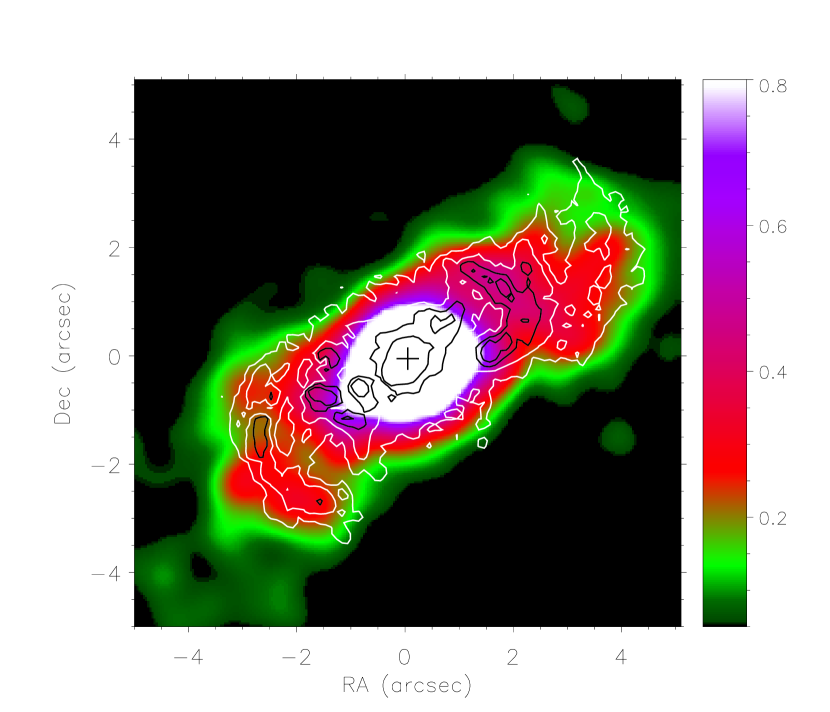
Figure 2.— Soft 0.2-2 keV ACIS/Chandra image of Mrk 573. (top): [O III] contours overlaid. (bottom): [O III]/$\rm{H\alpha}$ contours overlaid.

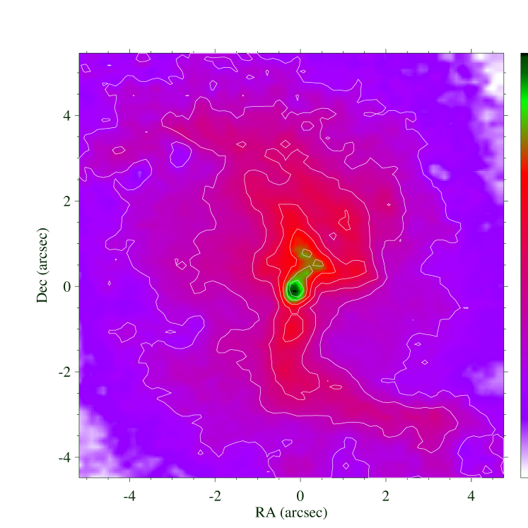
Figure 3.— I-H color map of Mrk 573. Left is the East and up is the North coordinates.

Two broad-band images using Chandra/ACIS data were created: (1) soft band at 0.2–2 keV, and (2) hard band at 2–10 keV. PSF simulations were carried out using information on the spectral distribution and off-axis location of the system as inputs to ChaRT PSF simulator. Hard band ($\sf{>}$2 keV) shows a point-like morphology, consistent with the FWHM PSF simulations, while soft band ($\sf{<}$2 keV) shows an extended morphology (see Figure 1).

The soft X-ray image shows a complex extended emission with a bipolar structure aligned along PA${\sf\sim 122^{\circ}}$ (Figure 2). It extends 8.5 arcsec to the NW and 6.5 arcsec to the SE. As already mentioned, Mrk 573 shows a biconical morphology in the [O III] emission, which resembles that observed in the soft X-rays.

The ratio of [OIII] to H recombination lines is commonly assumed to be an indicator of the ionization degree in line emitting photoionized gas. We have computed the [O III]/$\rm{H\alpha}$ map by dividing the flux-calibrated HST/WFPC2 images in those pixels where the signal-to-noise is higher than 3. A smoothing algorithm using the median within a box of 0.5 arcsec was then applied. Note that this ratio image is only used for morphological comparison and not for any quantitative analysis since the $\rm{H\alpha}$ image is contaminated with [N II] emission. The use of H$\alpha$ instead of H$\beta$ to compute the ionization map could be affected by reddening variations, as shown close to the nucleus of Mrk 573. However, the extinction map (Fig. 3) shows a very different morphology to that observed in the ratio [O III]/$\rm{H\alpha}$ map. This implies that the basic morphology of the optical ionization map cannot be explained by differential extinction, despite a certain fraction of the emission line map variations could be due to it.

The X-ray arc-like structure at 10 arcsec to the SE resembles the [O III] emission. However, the X-ray emission does not show the bridge between this structure and the inner parts of the SE cone seen in the [O III] image (also seen in [O III]/$\rm{H\alpha}$). The NW structure is coincident with the [O III] emission and strongly similar to the [O III]/$\rm{H\alpha}$ morphology (see Figure 2). These facts indicate a link between the soft X-ray emission and the optical ionized gas, although the detailed structure would depend on the small-scale ionization structure of the medium.

We have also explored the circumnuclear extinction. For this purpose we have used the broad-band images after subtracting the unresolved component to build a colour map of the circumnuclear region of Mrk 573. The colour map was created using the F814W and the F160W images, which are equivalent to the $I$ and $H$-bands, respectively. These filters were selected because they are not critically contaminated by emission lines, contrary to the colour maps presented by Quillen et al. (1999). The $I-H$ map covering the central 10 arcsec is shown in Figure 3. The reddest (or darkest in black/white) regions show the location of the strongest obscuration, or equivalently, the highest dust concentration. The colour map reveals a dust lane crossing the nucleus in the N–S direction, which bends after 2^′′ resembling incipient spiral arms. The axis delineated by this structure is oriented at about $55^{\circ}$ with respect to the alignment of the radio structure (Falcke et al., 1998; Kinney et al., 2000, PA $\sim 125^{\circ}$). The radio and the dust lanes axis should be almost perpendicular if the dust lanes were the outer parts of the postulated dusty torus for Type-2 nuclei. However, this is not necessarily the case, since the dust lane is observed at much larger scale than that of the postulated torus, changes in the dust plane may take place when approaching the inner nucleus. On the other hand, projection effects could mask the actual orientation of both structures, for instance Tsvetanov & Walsh (1992) proposed that the ionization cone is very inclined ($35^{\circ}$) with respect to the plane of the sky. In addition, there is also a tongue extending $0\farcs 5$ towards the N–NW which ends in two small blobs that resembles a structure observed in the excitation maps (see Figure 2). The presence of dust within the ionization cone has been reported before only in NGC 1068 (Bock et al., 2000). Towards the nucleus of the galaxy there is an excess of reddening which can be attributed to a natural increase in the extinction due to higher dust concentration. Assuming an intrinsic colour similar to that observed in the disk of galaxies ($\mathrm{I-H}\sim 2$; Moriondo et al., 1998), we have estimated a value of ${A_{V}=6.5}$ mag, which results in ${N_{H}=1.2\times 10^{22}}\mathrm{cm}^{-2}$.

Table 2Emission lines detected in the RGS/XMM-Newton spectrum.

Name	$\lambda_{rest}$	Energy	Flux
	(Å)	(keV)	$10^{-5}$
CV He$\gamma$	33.426	0.376	10.7$\,{}_{0.00}^{27.3}$
NVI He$\alpha$ (f)	29.534	0.420	0.00$\,{}_{0.00}^{82.7}$
NVI He$\alpha$ (i)	29.083	0.426	2.64$\,{}_{0.00}^{57.6}$
NVI He$\alpha$ (r)	28.787	0.431	0.00$\,{}_{0.00}^{1.85}$
CVI Ly$\beta$	28.466	0.436	3.18$\,{}_{0.57}^{7.10}$
NVII Ly$\alpha$	24.781	0.500	1.03$\,{}_{0.00}^{2.51}$
OVII He$\alpha$ (f)	22.101	0.561	5.17$\,{}_{2.33}^{9.21}$
OVII He$\alpha$ (i)	21.803	0.569	0.00$\,{}_{0.00}^{2.06}$
OVII He$\alpha$ (r)	21.602	0.574	3.76$\,{}_{0.96}^{7.58}$
OVIII Ly$\alpha$	18.969	0.654	2.17$\,{}_{1.00}^{3.70}$
OVII He$\gamma$	17.768	0.698	1.60$\,{}_{0.31}^{3.36}$
FeXVII 3s–2p	17.078	0.726	0.75$\,{}_{0.00}^{1.84}$
OVII RRC	16.771	0.739	1.07$\,{}_{0.03}^{2.65}$
FeXVII 3d–2p	15.010	0.826	0.65$\,{}_{0.02}^{1.45}$
OVIII RRC	14.228	0.882	0.48$\,{}_{0.00}^{1.33}$
NeIX(f)	13.698	0.905	0.22$\,{}_{0.00}^{0.94}$
NeIX(i)	13.552	0.915	0.12$\,{}_{0.00}^{1.10}$
NeIX(r)	13.447	0.922	0.76$\,{}_{0.08}^{1.87}$

Units are $\rm{ph~{}cm^{-2}~{}s^{-1}}$.

4. X-ray spectral analysis

X-ray spectral analysis of the observed soft X-ray extended emission is crucial to determine the excitation mechanism of the plasma, and its relationship to the optical bicone-like structure (see previous section). The combination of RGS/XMM-Newton high spectral resolution and ACIS/Chandra high spatial resolution data is key to achieve this purpose. In this section we describe in detail the methodology and main results obtained. In Section 5 we discuss the origin of this extended emission based on the results presented in this section. The analysis of the spectral counts was performed using the software package XSPEC (version 12.4.0; Arnaud, 1996).

Figure 4.— High resolution spectrum of Mrk 573 obtained with RGS/XMM-Newton instrument.

4.1. RGS/XMM–Newton high resolution spectra

Soft X-ray emission in Seyfert galaxies has been proven to consist of a plethora of emission lines plus a small fraction of continuum emission that can be described with a single flat power-law (Guainazzi et al., 2008) with a fixed spectral index of $\rm{\Gamma=1}$. We obtained the emission line fluxes of the central 30 arcsec region (note that this includes the nucleus and circumnuclear emission) using the RGS/XMM–Newton data. We searched for the presence of 37 emission lines of C, O, N, Si, Mg and Fe species by fitting the spectra of the two RGS cameras to Gaussian profiles together with a continuum. We used Cash statistic for this purposes.

The triplet fits were performed keeping the relative distance between centroids in energy and the centroid energy was left as a free parameter. A line was considered detected when the flux was higher than 0 at the 1${\sf\sigma}$ level. The resulting RGS spectrum and detected emission lines are presented in Figure 4 and Table 2, respectively. All energy centroids are consistent with the laboratory value given the error bars. Guainazzi et al. (2008) previously studied the RGS/XMM–Newton spectra of Mrk 573. Unfortunately, they only reported some of the lines, all of them agreeing with our emission line fluxes. The most intense emission lines comprising the RGS/XMM–Newton spectrum are: C VI Ly$\rm{\beta}$, O VII (r), O VII (f), O VIII Ly$\rm{\alpha}$, O VII H$\rm{\gamma}$, O VII RRC, Fe XVII 3d-2p, and Ne IX (r).

4.2. EPIC/XMM–Newton low resolution spectra

Figure 5.— Spectral fits (top panel) and residuals (bottom panel) for the nuclear spectrum of Mrk 573 using low resolution EPIC pn/XMM-Newton data. Dotted-lines show the Gaussian components used to fit the spectrum.

The fit of EPIC/XMM–Newton data with a thermal model produces poor results below 2 keV ($\sf{\chi^{2}}$ $\sim$16). Instead, a model composed of multiple emission lines was tried. Taking advantage of the RGS/XMM–Newton fit, we imposed that the intensity of the lines in the low resolution spectra fit do not exceed the RGS measurements. This is acceptable because the cross-calibrations between EPIC and RGS instruments shows a normalization constant in the range of 0.9 to 1.0 (see Plucinsky et al., 2008). The assumed Gaussian width is 100 eV. Note that for EPIC (and also ACIS/Chandra) data we do not question the existence of the emission lines detected on the RGS/XMM-Newton but we use them as a template. Triplets were fitted using the total flux of all components of the He-like lines O VII, N VI, and Ne IX. The continuum emission was fitted to a power-law to be consistent with the high spectral resolution analysis. However, this fit has poor statistics ($\rm{\chi^{2}_{r}>2}$). Five lines were added at energies above 0.95 keV in order to achieve an acceptable fit ($\rm{\chi^{2}_{r}=0.8}$): Fe XX at 0.97 keV ($\rm{\chi_{r}^{2}}$=5.64), Ne X Ly$\rm{\alpha}$ at 1.02 keV ($\rm{\chi_{r}^{2}}$=5.62), Ne IX He $\rm{\delta}$ at 1.16 keV ($\rm{\chi_{r}^{2}}$=3.72), Mg XI triplet at $\rm{\sim}$1.33 keV ($\rm{\chi_{r}^{2}}$=0.82), and Si XIII triplet at 1.84 keV($\rm{\chi_{r}^{2}}$=0.80). The final fit is shown in Figure 5. The low spectral resolution EPIC/XMM–Newton spectrum shows the following intense emission lines: C V He$\rm{\gamma}$, C VI Ly$\rm{\beta}$, N VII Ly$\rm{\alpha}$, O VII triplet, O VIII Ly$\rm{\alpha}$, O VII He$\rm{\gamma}$, O VII RRC, Fe XVII 3d-2p, and Ne IX triplet, Ne X Ly$\rm{\alpha}$, Ne IX He $\rm{\delta}$, and Mg XI triplet. In the best-fit model the flux of the OVIII RRC feature appears negligible and the adjacent line Fe XVII 3d2p is present. This is in contrast to what happens in the ACIS/Chandra nuclear spectrum (see Section 4.3 and Table 3). In order to check the compatibility of the results of both spectra, we have imposed a zero intensity to the line Fe XVII 3d2p finding a good fit. In this case, the OVIII RRC feature shows a similar flux compared to the flux reported using the Chandra nuclear spectrum. It is very likely that both features share the flux as measured in the RGS/XMM-Newton spectrum, although they cannot be distinguished in the low resolution spectra. The best-fit model has an absorbed 0.5-2.0 keV flux of F$\rm{{}_{0.5-2.0~{}keV}=}$3.38 (3.37-3.83) $\rm{\times 10^{-13}erg~{}s^{-1}~{}cm^{-2}}$, corresponding to an unabsorbed rest frame luminosity of L$\rm{{}_{0.5-2.0~{}keV}=}$2.0 (1.9-2.2) $\rm{\times 10^{41}~{}erg~{}s^{-1}}$. We have only included Galactic absorption in our model, which corresponds to $N_{H}=2.52\times 10^{20}$.

4.3. ACIS/Chandra spectra

We cannot separate the contribution of NW and SE regions to the RGS or EPIC/XMM–Newton spectra. However, this is possible by using the lower spectral resolution but better spatial resolution of ACIS/Chandra data.

We extracted spectra from the nucleus ($R=1$ arcsec) and two conical regions coincident with the extension of the emission, as seen in Figure 6. All extraction regions were centered at (RA, Dec)=01:43:57.78,+02:20:59.4. For the conical regions, we used an annulus, centered at the same position than the nucleus, with an inner and outer radius of 1.5 and 5 arcsec, respectively. The cones are defined by an opening angle of 60^o centered at $\mathrm{PA}=325^{\circ}$ (cone NW) and at $\mathrm{PA}=145^{\circ}$ (cone SE).

The study of the emission above 2 keV is beyond the scope of this paper since the nucleus dominates there and it has been already well studied before (Guainazzi et al., 2005). Therefore, channels above $\rm{\sim}$2 keV were ignored in the spectral fit. Again, the thermal model gives a poor fit with some residuals below 2 keV ($\sf{\chi^{2}}$ $\sim$3 for both cone regions).

We used the same model reported in the RGS/XMM–Newton spectrum assuming the emission line fluxes found in that case, as upper limits to fit the nucleus, and the NW and SE cone-like structures (the same as the EPIC/XMM–Newton data mentioned in the previous section). Moreover, the power-law component was removed in the cone-like structures because we expect this component to be detectable only in the nuclear region. The assumed Gaussian width is 100 eV. The spectra are shown in Figure 7 and final emission line fluxes are reported in Table 3.

Most of the emission lines in the EPIC/XMM–Newton spectrum are also detected in the nuclear spectrum using Chandra data (CV H$\rm{\gamma}$, N VII Ly$\rm{\alpha}$, O VII triplet, O VIII Ly$\rm{\alpha}$, Ne IX triplet, Ne X Ly$\rm{\alpha}$, and Mg XI triplet). Five of them were present only in the EPIC/XMM–Newton spectrum (C VI Ly$\rm{\alpha}$, O VII H$\rm{\gamma}$, O VII RRC, Fe XVII 3d-2p, and Ne IX He$\rm{\delta}$). We note that the flux measurements in the ACIS/Chandra spectrum are compatible with those of the EPIC/XMM-Newton including cases where only upper limits can be estimated in one of the spectra. In contrast with the EPIC/XMM–Newton spectrum, the Ne IX He$\rm{\delta}$ line at 1.16 keV was not needed, instead two more lines were added (Ne IX He$\rm{\gamma}$ and Ne X Ly$\rm{\gamma}$ at 1.13 and 1.22 keV, respectively) in order to get the best fit ($\sf{\chi^{2}}$=1.1). Note that in the case of Ne X Ly$\rm{\gamma}$ there are several transitions of Fe XX that could be contributing to this line. The inclusion of these two lines (i.e. Ne IX He$\rm{\gamma}$ and Ne X Ly$\rm{\gamma}$) instead of the Ne IX He$\rm{\delta}$ line also provides an aceptable fit to the EPIC/XMM–Newton spectrum. The line intensities are reported in Table 3 (within brackets). The final fit is equaly acceptable. A similar case is affecting the OVIII RRC and the Fe XVII 3d-2p lines (see Section 4.2).

Table 3Measured fluxes for EPIC/XMM-Newton and ACIS/Chandra spectra

Line	$\lambda_{rest}$	Energy	XMM-Newton	Chandra
				Nucleus	Cone NW	Cone SE
	(Å)	(keV)	($10^{-5}$)a	($10^{-5}$)a	($10^{-6}$)a	($10^{-6}$)a
Norm (pw)			$3.1_{2.4}^{3.7}$	$2.5_{2.2}^{2.9}$	…	…
${\sf CV~{}He\gamma}$	33.43	0.371	$18.6_{14.8}^{22.0}$	$12.1_{6.9}^{16.6}$	$12.6_{0.0}^{22.5}$	$27.9_{2.0}^{53.8}$
${\sf NVI~{}triplet}$	28.79/29.08/29.53	0.426	$0.9_{0.0}^{3.6}$	$2.5_{0.0}^{7.1}$	$1.5_{0.0}^{13.1}$	…
${\sf CVI~{}Ly\beta}$	28.47	0.436	$7.4_{1.7}^{9.4}$	$2.3_{0.0}^{5.6}$	$2.6_{0.0}^{10.6}$	…
${\sf NVII~{}Ly\alpha}$	24.78	0.500	$7.0_{5.7}^{8.3}$	$5.3_{4.4}^{6.6}$	$3.7_{0.0}^{7.6}$	$4.5_{1.0}^{7.9}$
${\sf OVII~{}triplet}$	21.60/21.80/22.10	0.569	$8.7_{7.5}^{9.9}$	$7.8_{6.4}^{9.2}$	$6.9_{5.0}^{10.9}$	$7.7_{3.2}^{12.2}$
${\sf OVIII~{}Ly\alpha}$	18.97	0.654	$3.5_{2.4}^{4.7}$	$2.3_{1.4}^{2.9}$	$0.5_{0.0}^{2.2}$	$1.5_{0.0}^{3.7}$
${\sf OVII~{}He\gamma}$	17.77	0.698	$1.2_{0.2}^{2.8}$	$0.0_{0.0}^{1.4}$	$0.0_{0.0}^{2.20}$	…
${\sf FeXVII~{}3s2}$	17.08	0.726	$1.2_{0.0}^{2.2}$	$1.6_{0.1}^{2.2}$	$2.4_{0.0}^{3.67}$	$1.7_{0.0}^{4.0}$
${\sf OVII~{}RRC}$	16.77	0.775	$1.0_{0.1}^{1.9}$	$0.8_{0.0}^{1.5}$	$1.8_{0.0}^{3.64}$	$1.6_{0.0}^{3.3}$
${\sf FeXVII~{}3d2p}$	15.01	0.826	$1.7_{0.7}^{2.2}$	$0.0_{0.0}^{1.7}$	$0.0_{0.0}^{2.89}$	…
${\sf OVIII~{}RRC}$	14.23	0.871	[$1.6_{1.0}^{2.0}$] b	$1.5_{0.0}^{2.6}$	$4.08_{0.43}^{5.15}$	$1.0_{0.2}^{1.8}$
${\sf NeIX~{}triplet}$	13.45/13.55/13.70	0.905	$2.5_{1.7}^{3.0}$	$2.2_{1.6}^{2.6}$	$0.0_{0.0}^{3.1}$	…
${\sf FeXX~{}3d2p}$	12.85	0.965	$0.1_{0.0}^{0.6}$	$0.32_{0.02}^{0.70}$	$0.76_{0.01}^{1.65}$	$0.6_{0.1}^{1.0}$
${\sf NeX~{}Ly\alpha}$	12.13	1.022	$1.3_{1.0}^{1.6}$	$1.1_{0.9}^{1.3}$	$1.3_{0.4}^{2.1}$
${\sf NeIX~{}He\gamma}$	10.97	1.130	[$0.7_{0.4}^{0.8}$] c	$0.44_{0.29}^{0.59}$	$0.7_{0.0}^{1.3}$	$0.9_{0.4}^{1.3}$
${\sf NeIX~{}He\delta}$	10.69	1.160	$0.8_{0.6}^{1.0}$	…	…	…
${\sf NeX~{}Ly\beta}$	10.16	1.220	[$0.3_{0.1}^{0.5}$] c	$0.33_{0.20}^{0.46}$	$0.13_{0.0}^{0.6}$	$0.02_{0.0}^{0.5}$
${\sf MgXI~{}triplet}$	9.17/9.31	1.352	$0.4_{0.2}^{0.6}$	$0.41_{0.30}^{0.52}$	$0.5_{0.2}^{0.8}$	$0.45_{0.2}^{0.7}$
${\sf SiXIII~{}triplet}$	6.65/6.74	1.840	$0.5_{0.0}^{2.8}$	$0.11_{0.02}^{0.19}$	$2.0_{0.9}^{3.1}$	…

Units are $\mathrm{ph}\,\mathrm{cm}^{-2}\,\mathrm{s}^{-1}$. This value was obtained by setting the nearby line FeXVII to zero. These values were computed after including Ne IX $\mathrm{He}\gamma$ and Ne X $\mathrm{Ly}\beta$, instead of NeIX $\mathrm{He}\delta$.

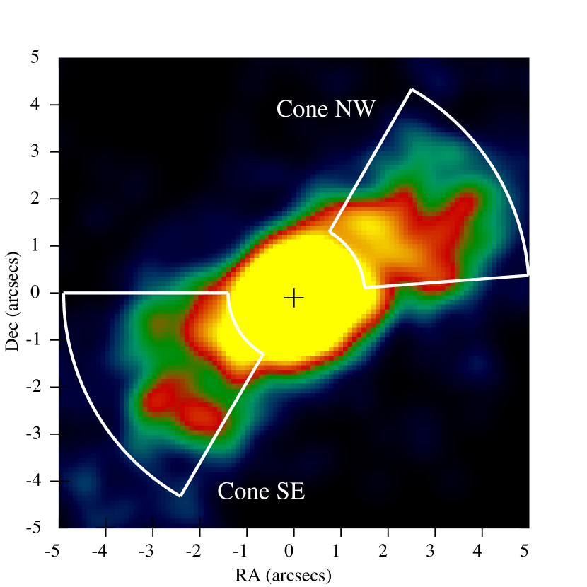
Figure 6.— Soft (0.2-2 keV) X-ray Chandra image with the two extracted regions (NW and SE) overplotted.

Figure 7.— Spectral fits ( top panels) and residuals ( bottom panels) using low resolution ACIS/Chandra spectra of the three regions: Nucleus (top), cone NW (middle) and cone SE (bottom).

The emission lines in the NW and SE cones are about a factor of 10 or more, fainter than those in the nuclear region using Chandra data. In the NW cone we have found the O VII triplet, O VIII RRC, Fe XX 3d2p, Ne X Ly$\rm{\alpha}$, Mg XI triplet and Si XIII triplet. A similar result is found in the SE cone with the detection of C V H$\rm{\gamma}$, N VII Ly$\rm{\alpha}$, O VII triplet, O VIII RRC, Ne IX triplet, Fe XX, Ne IX He$\rm{\delta}$, and Mg XI triplet. All of these lines were detected in the ACIS/Chandra nuclear region, except O VIII RRC.

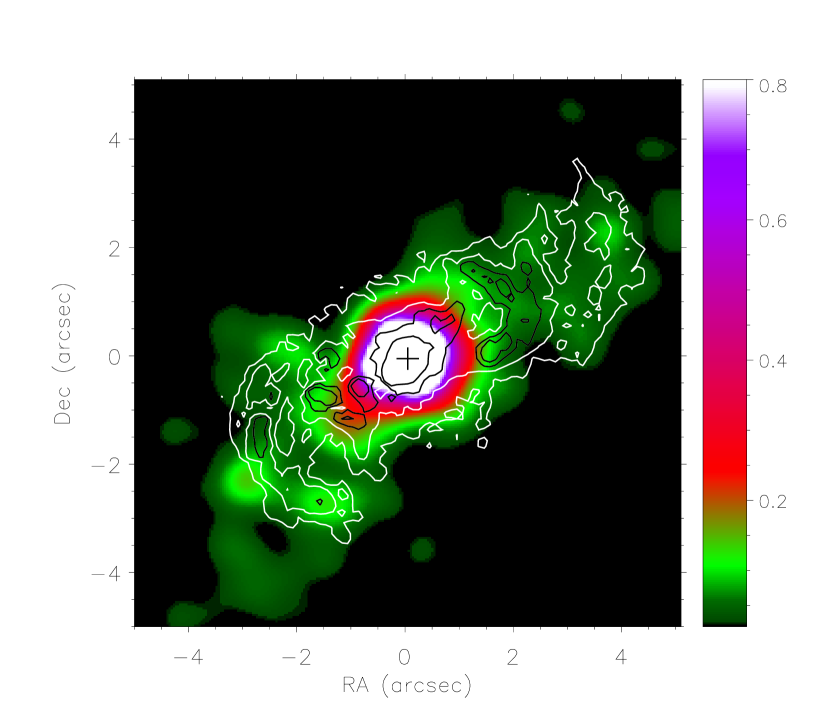
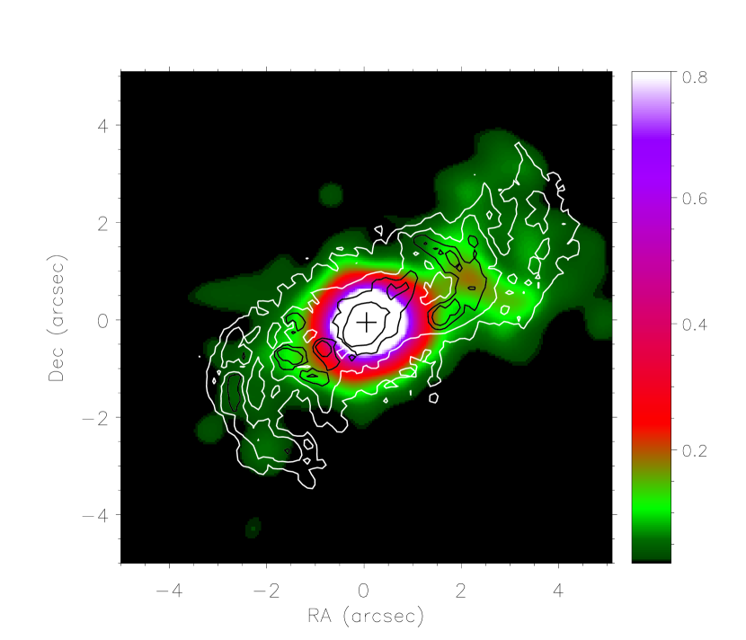
Figure 8.— Images centred at O VII triplet (top) and O VIII RRC (bottom) lines. [O III] contours are overlaid.

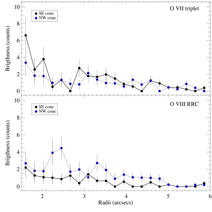
Figure 9.— Radial profile of the images centred at O VII triplet (top) and O VIII RRC (bottom) lines. Blue-dotted line and blue dots correspond to the NW cone while black-continous line and black dots correspond to the SE cone.

At first glance the spectra of the cones look rather different (see Figure 7), the NW cone spectrum shows an enhancement around 14Å(0.89 keV), which is not present in that of the SE cone. To illustrate this effect we have constructed two images centered at 0.5-0.7 keV and 0.8-1.0 keV, respectively (see Figure 8). These spectral intervals are dominated by the emission of the O VII triplet at 0.569 keV and O VIII RRC at 0.871 keV, respectively (see Tab. 3). The O VII triplet image shows a morphology similar to that found in the soft band ($\rm{<}$ 2 keV, see Figure 2). However, the O VIII RRC image shows a bright region to the NW of the nucleus. This can also be noticed in Figure 9 where the radial profiles of the O VII triplet and O VIII RRC images are plotted. The NW and SE profiles appear consistent in the case of the O VII triplet, whereas there is a clear bump at 2.5” in the NW side of the O VIII RRC profile compared to the SE one. Despite the limited signal-to-noise ratio of the spectra from the cones, it seems clear that the O VIII RRC is more important in the NW cone than in the SE cone (see Figs. 7 and 9).

5. Origin of the soft X-ray emission

As already said, the soft X-ray spectrum of Mrk 573 is dominated by line emission, as evident from the RGS/XMM–Newton data (Figure 4). Emission lines from H-like and He-like C, N, O, and Ne and Fe L-shell emission line Fe XVII dominate the spectrum, which also includes strong narrow RRC O VII and O VIII lines. The RRC features of these highly ionized species are produced when electrons recombine directly to the ground state. They are broad features for hot, collisionally ionized plasma, but are narrow, prominent features for photoionized plasma arising in low-temperature material (Liedahl & Paerels, 1996; Liedahl, 1999). Guainazzi & Bianchi (2007) measured in the Mrk 573 RGS spectrum the width of the RRC lines O VII and O VIII as $\rm{\sigma(O~{}VII)=3.5_{-3.3}^{+5.3}}$ eV and $\rm{\sigma(O~{}VIII)=4.8\pm 3.1}$ eV, respectively. These values indicates a relatively cool photoionized plasma.

Relative emission strength ratios of the He-like $\rm{1s2p~{}^{1}P_{1}\rightarrow~{}1s^{2}~{}^{1}S_{0}}$ (r, resonance), $\rm{1s2p~{}^{3}P_{2}\rightarrow~{}1s^{2}~{}^{1}S_{0}}$, $\rm{1s2p~{}^{3}P_{1}\rightarrow~{}1s^{2}~{}^{1}S_{0}}$ (i, blended inter-combinations) and $\rm{1s2s~{}^{3}S_{1}\rightarrow~{}1s^{2}~{}^{1}S_{0}}$ (f, forbidden) transitions can discriminate between photoionization, collisional excitation, or hybrid environment (Porquet & Dubau, 2000; Bautista & Kallman, 2000; Kahn et al., 2002). A weak resonance ($r$) line, compared to the forbidden ($f$) and intercombination ($i$) lines, corresponds to a pure photoionized plasma. A commonly used line ratio is defined as $G=(f+i)/r$. For Mrk 573 we measured a value of $G=1.4(0.3-12)$ for the ion O VII (see Tab. 2 and Figure 4). This value is lower than that expected for a pure photoionized plasma ($G>4$), but higher than that of collisional ionization. Such a value of G would indicate a hybrid plasma where collisional processes are not negligible (Porquet & Dubau, 2000), although the error bars do not allow a secure result. We could only obtain upper limits in the intensity of two of the lines needed to compute the $G$ ratio corresponding to the other ions (Ne IX and N VI) with detected He-like triplet transitions. The lower limit of G obtained using Ne IX ($\rm{(f+i)/r\gtrsim 2.7}$) is not conclusive although also points to an hybrib plasma. However, the use of $G$ ratios has been questioned by several authors (e.g. Kinkhabwala et al., 2002; Porter & Ferland, 2007). An important contribution of photoexcitation would rise the intensity of the resonance transition, which yields a decrease of the $G$ ratio relative to the pure photoionization case. Kinkhabwala et al. (2002) proposed the use of the ratio of higher order transitions to the forbidden triplet component in He-like ions as a good discriminant between photoexcitation and collisional ionization. Kinkhabwala et al. (2002) predicted a value of $\rm{F(O~{}VII~{}He\gamma)/F(O~{}VII~{}(He\alpha(f))}$ of 0.017 for collisional ionization. Thus, an excess of He$\gamma$ line relative to the forbidden transition, as measured in Mrk 573, $\rm{F(O~{}VII~{}He\gamma)/F(O~{}VII~{}(He\alpha(f))}$ $\rm{=0.31\,(0.03-1.4)}$ (see Tab. 2), indicates the importance of photoexcitation.

The intensities of the emission lines Fe XVII L (3d-2p) and Fe XVII K (3s-2p) are comparable in the case of Mrk 573 (see Tab. 2), which could be explained as an intermediate temperature plasma ($10\,\mathrm{eV}<\mathrm{kT}<500\,\mathrm{eV}$), or under hybrid conditions combining collisional and photoionization equilibrium conditions (Liedahl et al., 1990). Similarly, Sako et al. (2000) argued that the dominance of Fe XVII L lines can only be explained if photoexcitation by the nuclear radiation plays an important role, consistent with our suggestion throughout the G ratio.

From above, we conclude that the emission line diagnostics seems to indicate that the soft-X ray spectrum of Mrk 573 as seen by RGS/XMM-Newton data can be produced by a plasma dominated by photoionization and photoexcitation. Nevertheless, we cannot rule out some contribution of collisional excitation, based primarily on the presence of the Fe XVII 3d-2p transition. Unfortunately, the limited count level of the spectra does not permit us to give secure diagnostics. Detailed optical spectroscopic studies by Ferruit et al (1999) found that ionizing photons originating in the central source are not sufficient to explain the emission line luminosity. They suggest that fast shocks, associated with the jet/gas interactions, might contribute to the gas ionization.

The ACIS/Chandra spectrum of the nuclear region (1 arcsec) can be reproduced using the template obtained from the RGS/XMM–Newton analysis. The resulting fluxes are consistent with each other. Therefore, it seems that most of the emission line fluxes measured in the RGS spectra come from the inner central 2 arcsec region and is consistent with the photoionization and photoexcitation dominated plasma scenario.

NW cone emission differs from that of the SW cone and the nucleus. The O VIII RRC/O VII triplet ratio found in the NW cone ($\rm{F(OVIII~{}RRC)/F(O~{}VII(r,i,f))}$ $\rm{=0.6_{0.1}^{1.1}}$) is nominally higher than in the SE cone ($\rm{0.13_{0.02}^{0.56}}$) and in the nucleus ($\rm{<0.19}$), although consistent within the statistical uncertainties. According to Kinkhabwala et al. (2002) radiative decay following photoexcitation dominates the Seyfert 2 spectrum at low column densities, whereas recombination following photoionization dominates at high column densities. Following their prescription, the RRC intensity will increase compared to He-like triplet line when column density increases, which would imply a value of $\mathrm{N_{H}}$ larger for NW than for SE. Alternatively, the RRC line could be produced by hot collisionally ionized plasma, although the line widths reported by Guainazzi & Bianchi (2007) do not support this scenario. It is very unlikely that a broad feature contributes only in a few percentage of the total flux of source. Moreover, the radio maps of Mrk 573 are not sensitive enough to show great detail concerning radio emission although two faint blobs are observed in the NW cone (Falcke et al., 1998). The low signal-to-noise ratio of the spectra from the cones prevents us from a more detailed study of the line transitions in the extended emission.

5.1. Comparison with photoionization models

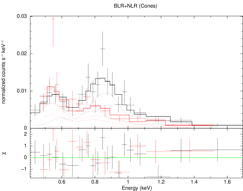
Figure 10.— (Top): ACIS/Chandra spectral fit and residuals to BLR+NLR Cloudy model of the nuclear region. (Bottom): Same for the cone-like regions. Red (black) crosses and red (black) continuous line are the NW (SE) cone spectrum and fit, respectively.

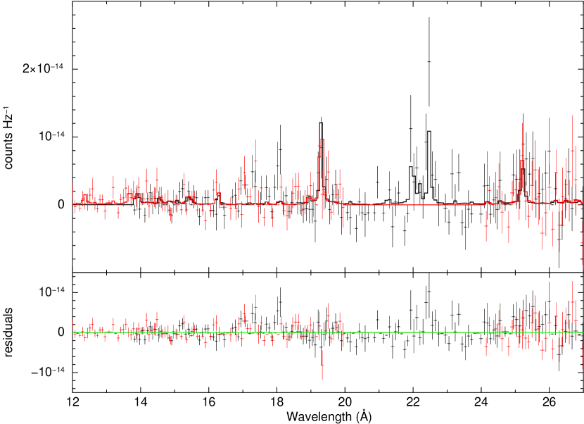
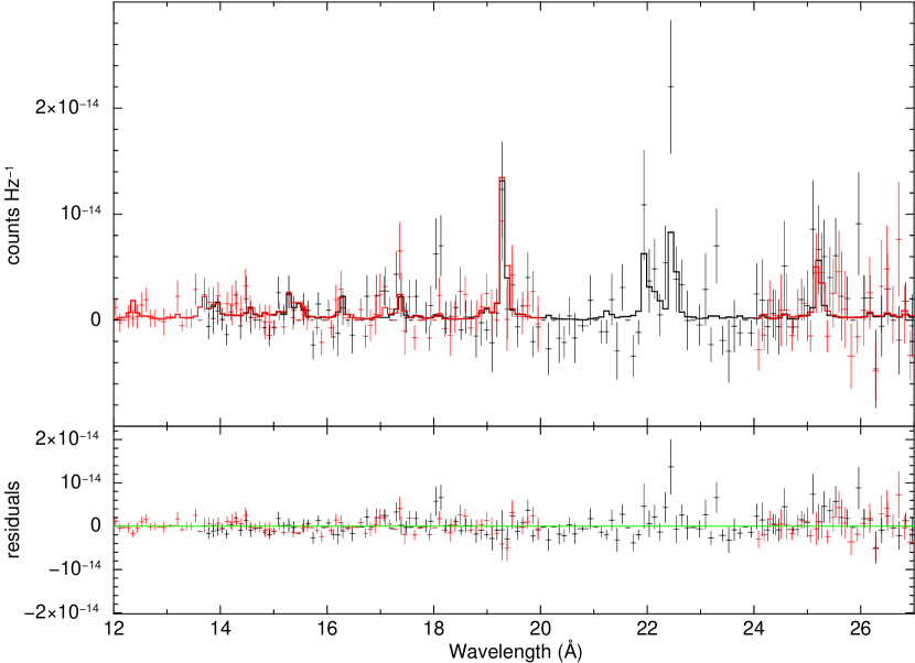
Figure 11.— (top): RGS/XMM-Newton spectra fitted to the best fit found for ACIS/Chandra spectrum of the nuclear region (see Figure 10). (bottom): Same than top figure but with the inclusion of the thermal model APEC with kT=0.4$\rm{\pm 0.1}$ keV.

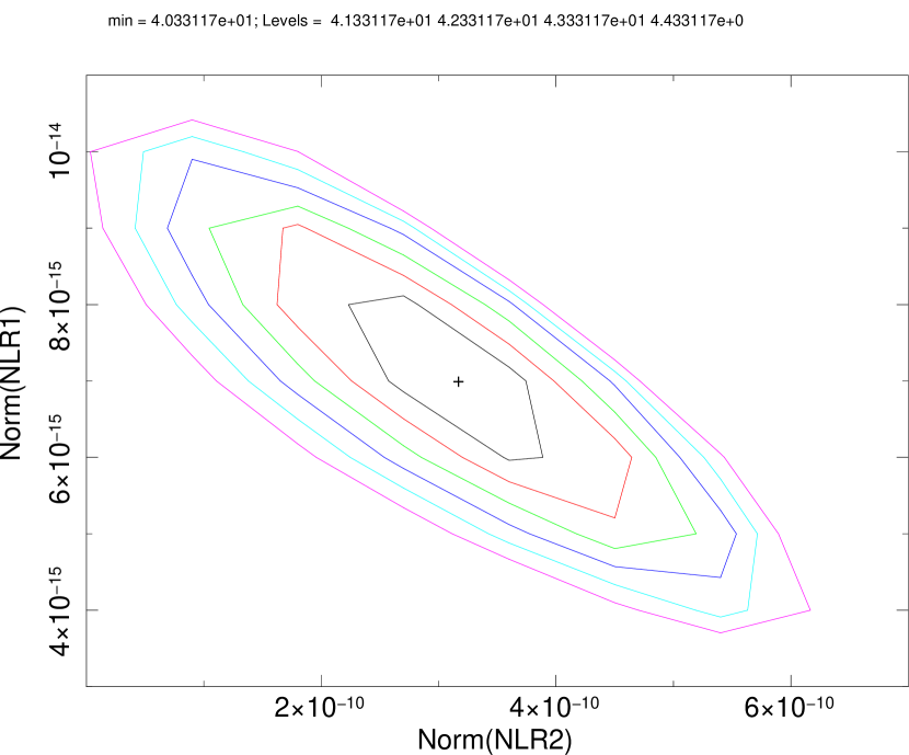
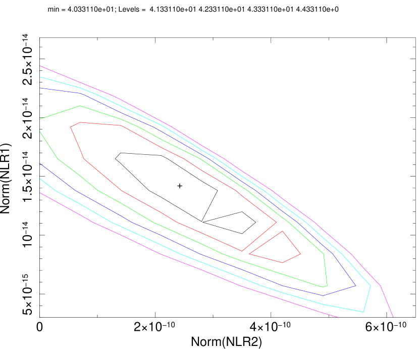
Figure 12.— 2-D iso-chi-squared flux contours of the normalization parameters of the best-fit Cloudy model of the reflected components of the NW (top) and SE (bottom) cones.

Using version c08.00 of the Cloudy package (last described by Ferland et al., 1998), we attempted to reproduce the observed spectra of the nuclear region and NE and SW cones seen in ACIS/Chandra data.

In these Cloudy simulations we assumed the source of ionization to emit as a typical AGN continuum (we used the model AGN available in Cloudy) defined by a “big bump” of temperature $\mathrm{T}=10^{6}\rm{K}$, an X-ray to UV ratio $\rm{\alpha_{OX}=-1.15}$, plus a X-ray power-law of spectral index of $\rm{\alpha=-1.0}$. A plane–parallel geometry is assumed, with the slab depth controlled by the hydrogen column density parameter ($\rm{N_{H}}$).

Two grids of parameters were constructed to simulate the expected BLR and NLR conditions. For each of them, a grid of models was simulated by varying the ionization parameter (U), the density of the material ($\mathrm{n_{H}}$), and the hydrogen column density ($\rm{N_{H}}$). U ranges from $\rm{10^{-3}}$ to $\rm{10^{3}}$, $\rm{N_{H}}$ ranges from $\rm{10^{20}\,cm^{-2}}$ to $\rm{10^{24}\,cm^{-2}}$ and $\mathrm{n_{H}}$ from $\rm{10^{9}\,cm^{-3}}$ to $\rm{10^{11}\,cm^{-3}}$ for BLR conditions, and from $\rm{10^{2}\,cm^{-3}}$ to $\rm{10^{4}\,cm^{-3}}$ for NLR conditions.

In both BLR or NLR models the outputs of each Cloudy simulation include a transmitted and a reflected emission line spectra. Under the Cloudy terminology “reflected” spectrum refers to the emission escaping into the $2\pi$ sr subtended by the illuminated face towards the ionizing source and by “transmitted” the emission escaping in the opposite direction. Each transmitted or reflected simulated emission line spectrum is imported as additive tables (“atable”) in XSPEC following Porter et al. (2006) procedure. All components are also absorbed through the Galactic value by using “wabs” on XSPEC. In practice, any additive table is included in XSPEC as follows: $\mathrm{wabs[N_{H}(Gal)](atable\{Cloudytable\}}$), where “Cloudytable” can be transmitted/reflected for BLR/NLR conditions.

Table 4Best fit parameters to a Cloudy BLR+NLR model. Nucleus and Cones.

	Nucleus		Cones (NW/SE)
Model param.	BLR	NLR	NLR 1	NLR 2
log(U)	$\rm{1.23_{1.18}^{1.27}}$	$\rm{0.13_{0.11}^{0.16}}$	$\rm{0.9\pm 0.3}$/$\rm{0.3\pm 0.2}$	-3∗/-3∗
log($n_{H})$	$\rm{9.8_{9.7}^{10.0}}$	$\rm{3.14_{3.10}^{3.18}}$	3∗	3∗
$\rm{log(N_{H})}$ [$\mathrm{cm}^{2}$]	$\rm{20.6_{20.5}^{20.7}}$	$\rm{20.6_{20.5}^{20.7}}$	20∗	20∗
Flux(0.5-2.0 keV) (trans.)	$\rm{35.8\pm 9.6}$	0.0 ($\rm{<6.6}$)	0.0 ($\rm{<5.3}$) / 9.3 ($\rm{<11.6}$)	3.4 ($\rm{<10.9}$) / 3.1 ($\rm{<9.3}$)
Flux(0.5-2.0 keV) (reflec.)	$\rm{61.1\pm 9.9}$	$\rm{92.6\pm 3.7}$	14.0 ($\rm{4.6-23.0}$) / 0.0 ($\rm{<14.5}$)	3.8 ($\rm{<10.9}$) / 3.0 ($\rm{<9.3}$)

For the nuclear region, neither BLR nor NLR models produced any acceptable fit ($\rm{\chi^{2}_{r}=1.9}$ and $\rm{\chi^{2}_{r}=1.8}$, respectively). Qualitatively, the issue is that BLR and NLR models alone failed in reproducing the relative strength between 0.55 keV (the O VII triplet) and 0.9 keV (the O VIII RRC and/or Ne IX triplet). We have found that the result of our Cloudy simulations do not change with the value of the volume density and column density in the range considered here. The models are mostly sensitive to the value of the ionization parameter. Besides the two simulations for BLR and NLR conditions (hereinafter called BLR and NLR models), we have also tried to model the spectrum of the nucleus as a combination of both BLR and NLR conditions (hereinafter BLR+NLR model). In the BLR+NLR model we use them all together, being then two transmitted and two reflected emission line spectra. The combination of BLR+NLR model produced a good fit (see Figure 10) with $\rm{\chi^{2}_{r}=1.3}$. The parameters of the best fit are given in Table 4. The modelled nuclear spectrum is equally dominated by the BLR and NLR emission (BLR is $\rm{\sim}$54% of the emission). We emphasize that in our simulation the use of a BLR component does not necessarily implies high density material, it rather accounts for ionization conditions higher than those of the NLR component.

In principle we could also expect some contribution from collisionaly ionised plasma (see Section 5). However, we know that this contribution should be small as indicated by the G ratios, and discussed in previous section. As an additional check, we used then this best-fit solution in order to reproduce the RGS/XMM-Newton spectra. We froze all the parameters adding a constant to the fit since we were mainly interested to check whether this model could reproduce the high resolution RGS spectra. We preferred this approach of fitting first the low resolution spectrum and taking this as a starting point to model the high resolution spectra. The final fit is given in Figure 11 (top) with a constant value of $\rm{1.2\pm 0.2}$. It gives a good representation of the data although it fails in reproducing the Fe XVII emission lines. Actually the inclusion of a thermal model (APEC) with a kT=0.4$\rm{\pm 0.2}$ keV reproduces better these features ($\rm{\Delta C\sim 14}$, see Figure 11 bottom). In the later case, it becomes very complex to discriminate between fits due to the low count level present in the high resolution spectrum. Based on this result, we went back to the low resolution data and try to fit the Chandra nuclear region adding the APEC component. Although it does not give formally a better fit, we obtained a fraction of the thermal component of $\rm{\sim}$ 6% of the total nuclear flux. This results confirms that the thermally ionized component is present, although its contribution is small.

We have also modelled the extended emission using the grid of Cloudy simulations. In this case we have to include the contamination from the PSF wings of the nuclear source. For this, we have computed the expected fraction of the nuclear flux contributing to the cone-like regions as $F\rm{{}_{nuc2cone}}=$$Flux_{PSF}\mathrm{(cone)}$$/Flux_{PSF}$ $\mathrm{(nucleus)}$. Assuming a Gaussian profile for the Chandra PSF with a FWHM of 1.2 arcsecs (see Figure 1), the fraction of nuclear spectrum contributing to the cone is $F\rm{{}_{nuc2cone}}=0.006$. This factor is equivalent to an integrated flux of F(0.5-2.0 keV)= $\rm{5.06\times 10^{-16}~{}erg~{}cm^{-2}s^{-1}}$, which corresponds to 2.5 and 3.5% of the NW and SE cone fluxes, respectively. In order to account for this nuclear contribution we have used the BLR+NLR best fit model found for the nucleus with all the parameters frozen, and scaled by the factor F_nuc2cone. Initially we have tried to fit the cone emission by a single phase medium, using Cloudy models with NLR conditions and both reflection and transmission components. Both NW and SE cones have been fitted simultaneously, although the normalizations of the reflection and transmission components for the two cones are let to vary independently. The hydrogen column density and density of the material have been frozen at log($\rm{N_{H}}$)=20 and log($\rm{n_{H}}$)=3 for simplicity. We recall that the simulated spectra by our Cloudy models are not sensitive to the value of these parameters within the explored range. The best fit show ionization parameters of log(U)=0.71$\rm{\pm}$0.07 and log(U)=0.13$\rm{\pm}$0.09 for NW and SE cones, respectively. Nevertheless, this fit failed to simultaneously reproduce the two spectra, being the statistics rather poor ($\rm{\chi^{2}_{r}=1.6}$). A much better fit is obtained ($\rm{\chi^{2}_{r}=1.1}$) if we add to this phase (hereinafter NLR1) a second one (hereinafter NLR2) with NLR conditions but a lower value of the ionization parameter U. We note that due to convergence problems within XSPEC we had to freeze the ionization parameter of the second phase. We checked that the best fit is obtained for a value of log(U)$\simeq\,-3$, in both regions. The ionization parameters for the NLR1 phases are log(U)=0.9$\rm{\pm}$0.2 and log(U)=0.3$\rm{\pm}$0.2 for NW and SE cones, respectively. These values are consistent with the parameters of the previous model. The final fit can be seen in Figure 10 and the best fit parameters and fluxes for each model component are given in Table 4. In order to show the confidence level of the fluxes, Fig. 12 includes the iso-chi-squared flux contours of the normalizations of the two phases (i.e. NLR1 and NLR2) of the reflected components for the NW (top) and SE (bottom) cones. Similar result is obtained for the transmitted components. The NLR1 phase mostly contributes to the X-ray spectrum at the region between 0.8-0.9 keV and 0.53-0.7 keV, whereas the NLR2 phase contributes at 0.52 and 0.7-0.85 keV. The lowest value of the ionization parameter is very similar to that required to fit the optical spectrum of Mrk 573 (Kraemer et al., 2009). In that work, the authors claimed a three phase component to explain the optical emission line spectrum. The low-ionization gas accounts for the [OII]$\rm{\lambda\lambda}$3727Å and [NII]$\rm{\lambda\lambda}$6548, 6584Å emission, whereas the moderately ionized phase accounts for the [OIII]$\rm{\lambda\lambda}$5007Å. Nonetheless, our NLR1 exhibits a value of U higher than their highly ionized phase. In addition, we expect a contribution of collisionaly ionized plasma (see Section 5) to be present in the extended emission. However, given the fact that its contribution to the nuclear spectrum is about 6%, we assumed its contribution to the extended emission to be equal or smaller than in the nuclear case and did not try any fit given the low count level in these regions.

In terms of flux, the NLR1 phase is the 64% of the extended emission flux. Its contribution in the NW cone is higher than in the SE cone. Moreover, the reflection component dominates the NW cone whereas the transmission component dominates the SE one. Tentatively, one could attribute this result to an orientation effect, being the NW cone located in the farthest side and the opposite for the SE one. Indeed, 2-D spectroscopic observations (Ferruit et al, 1999) indicates that at least part of the NW cone ionized gas is red-shifted with respect to the systemic velocity. This could indicates that NW cone axis could be oriented behind the sky plane, although close to it. This orientation apparently contradicts the orientation proposed by Tsvetanov & Walsh (1992) based on reddening measurements, although we remark that their findings refer to the orientation with respect to the galaxy disk, not to the sky plane. Remarkably, the NLR2 phase accounts for the same flux in the NW and SE cones and nearly equal relative contribution of the reflection and transmission components. Thus, this low ionization phase seems to be uniformly distributed along the cone area.

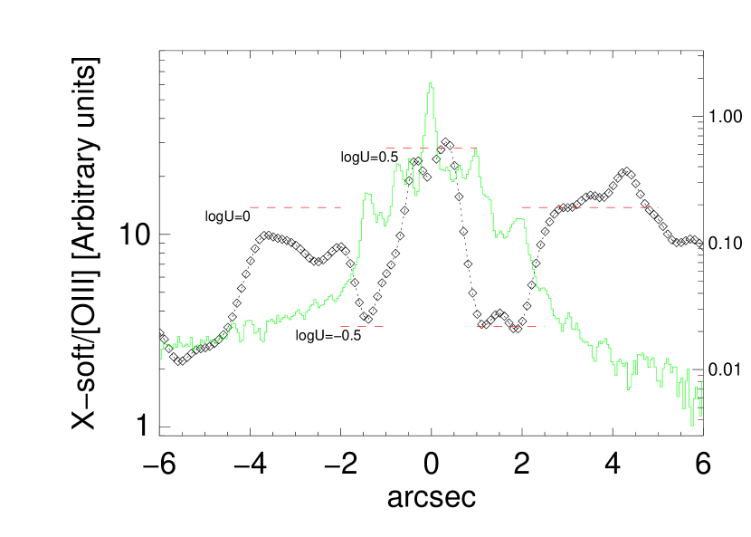
Figure 13.— Variation of the ratio of soft X-ray to [O III] brightness profile in arbitrary units. The [O III] brightness profile variation is also overploted as a green histogram-like line. Positive x-axis values indicates the NW orientation and negative values the SE one. Horizontal dashed lines represent predictions from simple photoionization models at various values of the ionization parameter.

At this point, we may conclude that soft extended X-ray emission is then powered by features coming from ionized gas in two phases under NLR-like conditions. Furthermore, one may question: is the [O III] extended emission structure powered by the same mechanism? The similarity between the [O III] structures and the soft X-ray emission points to a common origin for both components. We have investigated the radial variation of the ratio between the soft X-ray and the [O III] line emission. We represented in Figure 13 the variation of the brightness ratio along the axis of the cone ($\mathrm{PA}=122^{\circ}$). The brightness profiles were extracted using the IRAF pvector task. Before obtaining the ratio we convolved the [O III] profile to obtain the resolution of X-ray data. As can be seen from Figure 13 the ratio soft-X/[O III] presents a non-uniform variation showing a maximum at the nucleus; it then drops dramatically at the position of the [O III] arcs and returns at roughly half of the nuclear value outside the [O III] arcs. A similar behaviour, namely a small variation of the ratio, has been reported by Bianchi et al. (2006) for the case of NGC 3393. We have also compared the radial variation with predictions from photoionization models in Figure 13. We have used simple models assuming single plane–parallel slabs, constant density and radiation bounded clouds. The soft X-ray emission has been taken as the sum of the predicted values for the most intense features identified in our X-ray spectra. We have scaled the model predictions to the observed nuclear values from the model with $\rm{logU=0.5}$, which is close to the best fitting value derived above. The predictions for different values of the ionization parameters are represented in Figure 13. It can be seen that a variation of $U_{t}$ by one order of magnitude is needed to reproduce the observed variation in the brightness ratio from the nucleus to the arcs, which could be attributed to a combination of radiation dilution plus density enhancements at the arc positions. Note, that these variations are qualitatively in agreement with our Cloudy model simulations in which two different U values are needed for SE and NW cones. A baseline model where the density decreases as $r^{-2}$, as proposed by Bianchi et al. (2006), is compatible with our results, except for the regions close to [OIII] arcs. It is very likely that simple photoionization models are not adequate to reproduce the observed ionization variations, although a more sophisticated treatment must wait until higher quality X-ray spectroscopic observations become available. The fact that ionization- and matter-bounded clouds are likely constituents of the NLR has not been explored to explain emission lines in the soft-X range.

6. The Nuclear Spectral Energy Distribution

Figure 14.— High spatial resolution nuclear SED of Mrk 573 fitted with the clumpy torus models. Solid and dashed lines are the best fitting model and that computed with the median of each of the six parameters that describe the models (see Ramos Almeida et al. 2009b). The shaded region indicates the range of models compatible with a 68% confidence interval around the median.

Another important feature of the unified model is the optically thick torus. Under this scheme, Type-2 Seyferts like Mrk 573 are obscured due to this material located along our line of sight. The best way to study and characterize the molecular torus is by modeling the nuclear spectral energy distribution (SED) of the sources. The near- and mid-IR nuclear emission of Seyfert galaxies is attributed to the reprocessing of the UV/X-ray nuclear radiation by the toroidal dusty structure. For this reason, the infrared range is key to put constraints on torus modeling. However, in comparing the predictions of any torus model with observations, the small-scale torus emission must be isolated, in order to avoid contamination from the host galaxy. For this reason, it is important to use high angular resolution data when trying to model the torus emission.

We have tried here to explain the optical/infrared nuclear SED of Mrk 573 constructed with high spatial resolution data (see Table 1) using an interpolated version of the recent models for the clumpy torus scenario by Nenkova et al. (2008a, b). We have searched for the best fitting models using the Bayesian inference tool BayesClumpy (Asensio Ramos & Ramos Almeida, 2009) The results of the fit are shown in Figure 14.

Indeed, the nuclear SED of Mrk 573 has been previously fitted by Ramos Almeida et al. (2009b) using this set of models and tools, although the data points below 1 µm were not included in their analysis. For using the optical photometry derived in this work, the clumpy torus model fit needs an additional extinction factor, which is included as a foreground extinction. The derived median value is $A_{V}=7.3\pm 0.5$ mag, which can be translated to a column density of $\rm{N_{H}=1.39\times 10^{22}~{}\mathrm{cm}^{-2}}$. This value is nicely consistent with that derived from the optical colour–colour maps (see Sect. 3).

The results of the fitting process are the probability distributions for the free parameters that describe the clumpy models (see Ramos Almeida et al. 2009b). For Mrk 573, the median values of the parameters correspond to a torus width of 30^∘, $N_{0}=4\pm 1$ clouds in the equatorial direction, optical depth per single cloud $\tau_{V}\sim 60$, and $\mathrm{A_{V}^{LOS}}\sim 300$ mag (equivalent to $\mathrm{N_{H}^{LOS}}\sim 5.7\times 10^{23}~{}\mathrm{cm}^{-2}$). These torus parameters are similar to those derived without including the optical data points by Ramos Almeida et al. (2009b).

We have determined the torus luminosity integrating the corresponding emission from the torus model corresponding to the median value of the probability distribution of each parameter (dashed line in Figure 14). The resulting value is L${}_{bol}^{tor}=7.4\times 10^{43}~{}\mathrm{ergs^{-1}}$. The clumpy model fit yields the bolometric luminosity of the intrinsic AGN, L${}_{bol}^{AGN}=5.2\times 10^{44}~{}\mathrm{ergs^{-1}}$ (the bolometric luminosities are good to a factor of 2). Combining this value with the torus luminosity, we derive the reprocessing efficiency of the torus, which for Mrk 573 results to be quite low, about 14%.

Moreover, we have derived the X-ray luminosity from the hard X-ray part, assuming a power law with photon index 1.8. The range from 2 to 6 keV was used to avoid, on the one hand the soft range, which is attributed to emission lines, and the Fe K-line on the other. The galactic absorption plus an intrinsic absorption were included in the fitting process. The intrinsic absorption results in a value of $\mathrm{N_{H}}=7_{-5}^{+6}\times 10^{22}~{}\mathrm{cm}^{-2}$, which is compatible with the foreground extinction inferred from the colour maps and the clumpy torus modeling. Thus, the absorption corrected X-ray luminosity is $\mathrm{L_{2-10~{}keV}}=1.7\times 10^{41}~{}\mathrm{erg\,s^{-1}}$. This value is quite low when compared to the optical/infrared luminosity reprocessed by the blocking torus. However, it can be reconciled by taking into account that Mrk 573 has been classified as a Compton-thick AGN (Guainazzi et al., 2005), and its X-ray luminosity has to be corrected by a large factor to obtain the intrinsic luminosity, since the column density is $\rm{N_{H}>1.6\times 10^{24}~{}cm^{-2}}$ (such high value of the optical depth is also consistent with the value derived above from the clumpy torus modeling). Panessa et al. (2006) derived a factor of 60 comparing a small sample of Compton-thick Type-2 Seyferts with a sample of Type-1 Seyferts, whereas Cappi et al. (2006) derived a factor about 100. These values are in contrast with the work of González-Martín et al. (2009), who obtained a value of 42 using a sample of LINERs. In addition, we have to transform from X-ray to bolometric luminosity multiplying by a factor 30 (Risaliti & Elvis 2004; see also Panessa et al. 2006). Thus, we obtain a value for the bolometric AGN luminosity in the range $\mathrm{L^{bol}_{AGN}=3.1-5.1\times 10^{44}~{}ergs^{-1}}$, which is in nice agreement with the value derived from the torus reprocessing, given the uncertainties involved. Kraemer et al. (2009) derived a higher value for the bolometric luminosity ($3.2\times 10^{45}~{}ergs^{-1}$) based on the [OIV] 25.9µm luminosity, as measured by the Spitzer/IRS spectrum of Mrk 573 (Meléndez et al., 2008a, b). In any case Mrk 573 seems to be radiating near to the Eddington limit assuming the black hole mass to be around $2\times 10^{7}\mathrm{M_{\odot}}$ (Bian & Gu, 2007). This result adds support to the re-classification of Mrk 573 as a hidden narrow-line Seyfert 1 (Ramos Almeida et al., 2008).

7. Conclusions and overall picture

Mrk 573 is a nearby optically classified Type-2 Seyfert, well-known for its extended circumnuclear emission-line regions. It is this extension and the proximity of the source that convert Mrk 573 as one of the ideal cases to study this emission commonly found in Type-2 Seyfert galaxies. We combine RGS/XMM-Newton and ACIS/Chandra to achieve high spectral and spatial resolution in order to disentangle the emission mechanism of this extended emission. We also used optical and near-IR HST data in order to compare with the X-ray data. The main results are:

• The soft X-ray emission is very complex, resembling that of the [O III] emission, as already reported. What constitutes a new result is that especially the NW structure is also very similar to that of [O III]/$\rm{H\alpha}$ emission. This suggests the same origin for the emission lines at optical and the soft X-ray ranges.

• Through X-ray spectroscopic analysis we have found that plasma excitation mechanism in the nuclear spectrum is mainly driven by photoionization from the central source, including a strong contribution from photoexcitation. A small contribution of collisionally ionized plasma is also needed to explain the emission line ratios shown by RGS spectra. This conclusion also agrees with the proposed Cloudy simulations since the spectra could be interpreted as the combination of two different phases of Cloudy models, with two different ionization parameters log(U)=1.23 and log(U)=0.13.

• Based on the ACIS/Chandra images and radial profiles along O VII triplet and O VIII RRC for cone-like structures we showed that O VIII RRC could be more relevant toward the NW cone, although the line ratios are formally compatible after including the error bars.

• We have successfully modelled the cone-like emission using Cloudy simulations corresponding to two phases of NLR conditions. The first phase shows different values of ionization parameter and different contributions of the reflected and transmitted components for the NW (log(U)=0.9, reflected dominated) and SE ( log(U)=0.3, transmitted dominated) cones. The second is an homogeneous phase with a lower ionization parameter (log(U)=-3) and the same contribution of reflected and transmitted componets for NW and SE cones.

• We have found a good agreement between the AGN bolometric luminosity derived from the hard X-ray luminosity and the one derived from the modeling of the optical/infrared SED with a clumpy torus model.

• From the extinction maps we have found that a dust lane crosses the nucleus in the N–S direction. This could be, in projection, perpendicular to the direction of the cone-like structure. The amount of extinction we have derived from this map is also consistent with that derived from the SED modeling. However, this must be related with the extended extinction since, in the inner parts, the AGN is hidden by a column density on the Compton-thick regime ($\rm{N_{H}>1.6\times 10^{24}cm-2}$).

Note added in manuscript: After this paper was submitted to the journal a paper was published by Bianchi et al. (2010) with data in common with our work. Most of their results are consistent with ours, although different approaches were used. They fitted the XMM-Newton/RGS spectra using Cloudy photoionization models. Their best fit was obtained by an hybrid model -photoionization + collisional excitation- where the collisional phase contributes 1/3 of the flux in the band 0.5-0.8 keV, consistent with our work. Moreover, they claimed the need of two photoionization phases (log U = 0.3 and 1.8) to explain the ACIS/Chandra spectrum in the range 0.4-7 keV, which is also in agreement with our results. The results on the extended emission cannot be compared since they do not distinguish between the two cone-like structures, extracting the spectrum from a circumnuclear annulus.

References

- Antonucci (1993) Antonucci, R. R. J. 1993, ARA&A, 31, 473
- Alonso-Herrero et al (2003) Alonso-Herrero A., Quillen, A. C., Rieke, G. H., Ivanov, V. D., & Efsthatiou A. 2003 AJ, 126, 81
- Arnaud (1996) Arnaud, K. A. 1996, Astronomical Data Analysis Software and Systems V, 101, 17
- Asensio Ramos & Ramos Almeida (2009) Asensio Ramos, A., & Ramos Almeida, C. 2009, ApJ, 696, 2075
- Bautista & Kallman (2000) Bautista, M. A., & Kallman, T. R. 2000, ApJ, 544, 581
- Bian & Gu (2007) Bian, W., & Gu, Q. 2007, ApJ, 657, 159
- Bianchi et al. (2010) Bianchi, S., Chiaberge, M., Evans, D. A., Guainazzi, M., Baldi, R. D., Matt, G., & Piconcelli, E. 2010, MNRAS, 405, 553
- Bianchi et al. (2006) Bianchi, S., Guainazzi, M., & Chiaberge, M. 2006, A&A, 448, 499
- Bock et al. (2000) Bock, J. J., et al. 2000, AJ, 120, 2904
- Burrows et al. (2000) Burrows, D. N., et al. 2000, ApJ, 543, L149
- Cappi et al. (2006) Cappi, M., et al. 2006, A&A, 446, 459
- Crenshaw et al. (2003) Crenshaw, D. M., Kraemer, S. B., & George, I. M. 2003, ARA&A, 41, 117
- Crenshaw et al. (1999) Crenshaw, D. M., Kraemer, S. B., Boggess, A., Maran, S. P., Mushotzky, R. F., & Wu, C.-C. 1999, ApJ, 516, 750
- Dai et al. (2008) Dai, X., Mathur, S., Chartas, G., Nair, S., & Garmire, G. P. 2008, AJ, 135, 333
- Ebeling et al. (2006) Ebeling, H., White, D. A., & Rangarajan, F. V. N. 2006, MNRAS, 368, 65
- Evans et al. (2006) Evans, D. A., Lee, J. C., Kamenetska, M., Gallagher, S. C., Kraft, R. P., Hardcastle, M. J., & Weaver, K. A. 2006, ApJ, 653, 1121
- Falcke et al. (1998) Falcke, H., Wilson, A. S., & Simpson, C. 1998, ApJ, 502, 199
- Ferland et al. (1998) Ferland, G. J., Korista, K. T., Verner, D. A., Ferguson, J. W., Kingdon, J. B., & Verner, E. M. 1998, PASP, 110, 761
- Ferruit et al (1999) Ferruit, P., Wilson, A. S., Falcke, H., Simpson, C., Pécontal E., & Durret, F., MNRAS, 309, 1
- Gabriel et al (2004) Gabriel, C., Denby, M., Fyfe, D.J. et al 2004, in Astronomical Data Analysis Software and Systems (ADASS) XIII, ASP Conf Ser., 314, 759
- González-Martín et al. (2009) González-Martín, O., Masegosa, J., Márquez, I., & Guainazzi, M. 2009, ApJ, 704, 1570
- Guainazzi et al. (2005) Guainazzi, M., Matt, G., & Perola, G. C. 2005, A&A, 444, 119
- Guainazzi & Bianchi (2007) Guainazzi, M., & Bianchi, S. 2007, MNRAS, 374, 1290
- Guainazzi et al. (2008) Guainazzi, M., Bianchi, S., Cappi, M., Dadina, M., & Malaguti, G. 2008, Revista Mexicana de Astronomia y Astrofisica Conference Series, 32, 96
- Hopkins et al. (2006) Hopkins, P. F., Robertson, B., Krause, E., Hernquist, L., & Cox, T. J. 2006, ApJ, 652, 107
- Kahn et al. (2002) Kahn, S. M., Behar, E., Kinkhabwala, A., & Savin, D. W. 2002, Royal Society of London Philosophical Transactions Series A, 360, 1923
- Kauffmann et al. (2003) Kauffmann, G., et al. 2003, MNRAS, 346, 1055
- Kinney et al. (2000) Kinney, A. L., Schmitt, H. R., Clarke, C. J., Pringle, J. E., Ulvestad, J. S., & Antonucci, R. R. J. 2000, ApJ, 537, 152
- Kinkhabwala et al. (2002) Kinkhabwala, A., et al. 2002, ApJ, 575, 732
- Kraemer et al. (2008) Kraemer, S. B., Schmitt, H. R., & Crenshaw, D. M. 2008, ApJ, 679, 1128
- Kraemer et al. (2009) Kraemer, S. B., Trippe, M. L., Crenshaw, D. M., Meléndez, M., Schmitt, H. R., & Fischer, T. C. 2009, ApJ, 698, 106
- Krist (1993) Krist, J. 1993, Astronomical Data Analysis Software and Systems II
- Liedahl et al. (1990) Liedahl, D. A., Kahn, S. M., Osterheld, A. L., & Goldstein, W. H. 1990, ApJ, 350, L37
- Liedahl (1999) Liedahl, D. A. 1999, X-Ray Spectroscopy in Astrophysics, 520, 189
- Liedahl & Paerels (1996) Liedahl, D. A., & Paerels, F. 1996, ApJ, 468, L33
- Meléndez et al. (2008a) Meléndez, M., Kraemer, S. B., Schmitt, H. R., Crenshaw, D. M., Deo, R. P., Mushotzky, R. F., & Bruhweiler, F. C. 2008, ApJ, 689, 95
- Meléndez et al. (2008b) Meléndez, M., et al. 2008, ApJ, 682, 94
- Moriondo et al. (1998) Moriondo, G., Giovanelli, R., & Haynes, M. P. 1998, A&A, 338, 795
- Nenkova et al. (2008a) Nenkova, M., Sirocky, M. M., Nikutta, R., Ivezić, Ž., & Elitzur, M. 2008, ApJ, 685, 160
- Nenkova et al. (2008b) Nenkova, M., Sirocky, M. M., Ivezić, Ž., & Elitzur, M. 2008, ApJ, 685, 147
- Ogle et al. (2003) Ogle, P. M., Brookings, T., Canizares, C. R., Lee, J. C., & Marshall, H. L. 2003, A&A, 402, 849
- Ogle et al. (2000) Ogle, P. M., Marshall, H. L., Lee, J. C., & Canizares, C. R. 2000, ApJ, 545, L81
- Panessa et al. (2006) Panessa, F., Bassani, L., Cappi, M., Dadina, M., Barcons, X., Carrera, F. J., Ho, L. C., & Iwasawa, K. 2006, A&A, 455, 173
- Peng et al. (2002) Peng, C. Y., Ho, L. C., Impey, C. D., & Rix, H.-W. 2002, AJ, 124, 266
- Pogge & De Robertis (1993) Pogge, R. W., & De Robertis, M. M. 1993, ApJ, 404, 563
- Porquet & Dubau (2000) Porquet, D., & Dubau, J. 2000, A&AS, 143, 495
- Porter & Ferland (2007) Porter, R. L., & Ferland, G. J. 2007, ApJ, 664, 586
- Porter et al. (2006) Porter, R. L., Ferland, G. J., Kraemer, S. B., Armentrout, B. K., Arnaud, K. A., & Turner, T. J. 2006, PASP, 118, 920
- Plucinsky et al. (2008) Plucinsky, P. P., et al. 2008, Proc. SPIE, 7011,
- Quillen et al. (1999) Quillen, A. C., Alonso-Herrero, A., Rieke, M. J., McDonald, C., Falcke, H., & Rieke, G. H. 1999, ApJ, 525, 685
- Ramos Almeida et al. (2009a) Ramos Almeida, C., Pérez García, A. M., & Acosta-Pulido, J. A. 2009a, ApJ, 694, 1379
- Ramos Almeida et al. (2009b) Ramos Almeida, C., Levenson N. A., Alonso-Herrero A., Asensio Ramos A., Radomski, J. T., Packham C., Fisher R. S., & Telesco C. M. 2009b, ApJ, 702, 1127
- Ramos Almeida et al. (2008) Ramos Almeida, C., Pérez García, A. M., Acosta-Pulido, J. A., González-Martín, O. 2008, ApJ, 680, L17
- Ramos Almeida et al. (2006) Ramos Almeida, C., Pérez García, A. M., Acosta-Pulido, J. A., Rodríguez Espinosa, J. M., Barrena, R., & Manchado, A. 2006, ApJ, 645, 148
- Risaliti & Elvis (2004) Risaliti, G., & Elvis, M. 2004, Supermassive Black Holes in the Distant Universe, 308, 187
- Ruiz et al. (2005) Ruiz, J. R., et al. 2005, AJ, 129, 73
- Sako et al. (2000) Sako, M., Kahn, S. M., Paerels, F., & Liedahl, D. A. 2000, ApJ, 543, L115
- Schawinski et al. (2009) Schawinski, K., Virani, S., Simmons, B., Urry, C. M., Treister, E., Kaviraj, S., & Kushkuley, B. 2009, ApJ, 692, L19
- Schawinski et al. (2007) Schawinski, K., et al. 2007, MNRAS, 382, 1415
- Schlesinger et al. (2009) Schlesinger, K., Pogge, R. W., Martini, P., Shields, J. C., & Fields, D. 2009, ApJ, 699, 857
- Schmitt et al. (2003) Schmitt, H. R., Donley, J. L., Antonucci, R. R. J., Hutchings, J. B., & Kinney, A. L. 2003, ApJS, 148, 327
- Silk & Rees (1998) Silk, J. & Rees, M. J. 1998, A&A, 331, L1
- Strüder et al. (2001) Strüder, L., et al. 2001, A&A, 365, L18
- Tsvetanov & Walsh (1992) Tsvetanov, Z., & Walsh, J. R. 1992, ApJ, 386, 485
- van Dokkum (2001) van Dokkum, P. G. 2001, PASP, 113, 1420
- Veilleux et al. (2003) Veilleux, S., Shopbell, P. L., Rupke, D. S., Bland-Hawthorn, J., & Cecil, G. 2003, AJ, 126, 2185
- Whittle & Wilson (2004) Whittle, M. & Wilson, A. S. 1992, AJ, 127, 606
- Yang et al. (2001) Yang, Y., Wilson, A. S., & Ferruit, P. 2001, ApJ, 563, 124
- Young et al. (2001) Young, A. J., Wilson, A. S., & Shopbell, P. L. 2001, ApJ, 556, 6