Effect of scattering lengths on the dynamics of a
two-component Bose-Einstein condensate

Abstract

We examine the effect of the intra- and interspecies scattering lengths on the dynamics of a two-component Bose-Einstein condensate, particularly focusing on the existence and stability of solitonic excitations. For each type of possible soliton pairs stability ranges are presented in tabulated form. We also compare the numerically established stability of bright-bright, bright-dark and dark-dark solitons with our analytical prediction and with that of Painlevé-analysis of the dynamical equation. We demonstrate that tuning the inter-species scattering length away from the predicted value (keeping the intra-species coupling fixed) breaks the stability of the soliton pairs.

I Introduction

Since Bose-Einstein condensates (BECs) can be routinely prepared in laboratories, ultracold gases became a very important testbed for many predictions of condensed matter physics Bloch et al. (2008). The experimental examination of binary condensates started nearly the same time as for single condensates by using two different quantum states of the same species, such as ⁸⁷Rb Myatt et al. (1997) or ²³Na Stamper-Kurn et al. (1998). With the development of sympathetic cooling ultracold mixtures have been assembled from two different alkalies, ⁴¹K–⁸⁷Rb Modugno et al. (2001); Thalhammer et al. (2008), ⁷Li–¹³³Cs Mudrich et al. (2002) and ⁸⁷Rb–¹³³Cs Pilch et al. (2009) or for different isotopes of the same alkali atom ⁸⁵Rb–⁸⁷Rb Papp et al. (2008). The tunability of the inter- and intra-species scattering lengths via driving the mixture through a Feshbach-resonance has also been experimentally demonstrated Thalhammer et al. (2008); Pilch et al. (2009).

The ability to create Bose-Einstein condensate(s), a highly coherent form of matter, also facilitated the convergence of two fields of physics: condensed matter physics and quantum optics, and therefore BECs became favourable candidates for examining the effects of nonlinearity in matter waves, where this nonlinearity originates from the mean-field representation of the interatomic interaction. The similarity between electromagnetic waves in nonlinear medium and coherent matter waves is also expressed in the equations of motion which is the nonlinear Schrödinger equation (NLS) for the former and the Gross-Pitaevskii (GP) equation for the latter. Although the physical interpretation of these equations is different, their structures are the same apart from the external potential term. Furthermore, in some cases this extra term can even be removed Schumayer and Apagyi (2002) and the GP equation is transformed into a form coinciding with the NLS equation. Consequently all results for the NLS equation known in nonlinear optics can be readily adapted to Bose-Einstein condensates.

One of the surprising phenomena of nonlinear optics is the existence of particle-like wave-forms, the so-called solitons Hasegawa and Matsumoto (2002). Such excitations have already been experimentally observed in single- or two-component Bose-Einstein condensates: dark solitons Burger et al. (1999); Denschlag et al. (2000), bright solitons Khaykovich et al. (2002); Strecker et al. (2002), their two-component coupled analogues, the dark-dark Öhberg and Santos (2001), bright-bright Liu and Hao (2002) or even dark-bright Busch and Anglin (2001); Becker et al. (2008) multi-component solitary waves Ginsberg et al. (2005); Becker et al. (2008).

However, the question of existence of solitons needs more attention than simply recognising the similarity between the two governing equations. The existence of solitons is strongly related to the integrability of the given physical model. An usual test to determine whether or not an equation is integrable is the Painlevé-test (P-test) Steeb et al. (1984). It was shown that without any potential term or inhomogeneity the one-dimensional NLS equation, $iu_{t}+u_{xx}\pm 2\left|u\right|^{2}u=0$, is completely integrable both in its one-component Zakharov and Shabat (1972); Steeb et al. (1984) or multi-component Zakharov and Manakov (1974, 1985) form. However, the inclusion of a potential term, $v(x,t)u$, in the one-component NLS equation or different coupling strengths in the multi-component NLS/GP equations fundamentally changes their integrability Sahadevan et al. (1986); Clarkson (1988). It was shown that integrability is preserved provided the external potential, $v(x,t)$, has a specific form Clarkson (1988). The authors examined Schumayer and Apagyi (2001) the integrability of the two-component coupled Gross-Pitaevskii (CGP) equations and lead to similar conclusion: the scattering lengths and the external potentials cannot be arbitrary if the integrability of CGP is to be preserved. The inter- and intraspecies scattering lengths must satisfy the following equation

$$\frac{2\xi_{1}\xi_{2}-\kappa_{1}\xi_{1}-\kappa_{2}\xi_{2}}{\xi_{1}\xi_{2}-\kappa_{1}\kappa_{2}}=\!\frac{(2n+1)^{2}+7}{16},$$ (1)

where $\xi_{1}=a_{11}/a_{21}$, $\xi_{2}=a_{22}/a_{12}$, $\kappa_{1}=\mu_{11}/\mu_{21}$, $\kappa_{2}=\mu_{22}/\mu_{12}$ and $\mu_{ij}$ denotes the reduced mass of pair of particles composed by an atom from the $i$th and $j$th species. On the right hand side of Eq. (1) $n$ is a non-negative integer number. One may call $n$ a classification number, because it determines the form of the external potentials for which CGP equations remain integrable. For example, for $n=2$, the external potential, apart from the quadratic trapping potential, may even contain an imaginary time-dependent term Schumayer and Apagyi (2001). This term can mimic the loss or gain in the number of particles of the given species. We note here that usually dissipation works against long-living coherent matter waves, however, the importance of this imaginary potential term has been analysed in Brazhnyi et al. (2009); Rajendran et al. (2009) and shown to permit exact soliton solution Nakkeeran (2001). In the context of BECs at finite temperature, the interaction of the condensate with the thermal cloud could also be taken into account as an imaginary term in the governing GP equation. This interaction, due to its stochastic nature, can influence the dynamics of the solitons, via density-fluctuation.

In this paper we carry out an analysis on how the intra- and interspecies interaction influences the dynamics of a binary mixture of Bose-Einstein condensates. We select out of the many possible systems of two component BECs the pairs ⁸⁷Rb–⁸⁷Rb (prepared in two distinct hyperfine states), ²³Na–⁸⁷Rb, and ⁷Li–³⁹K. In the former two systems there is a possibility to study stability of bright-dark and dark-dark soliton pairs, while the last pair is capable to sustain bright-bright and bright-dark excitations.

The organization of the paper is as follows. Section II defines a quasi one-dimensional model derived from the general three-dimensional, coupled Gross-Pitaevskii equations assuming cigar-like harmonic oscillator trap potential. In the first part of section III we shall perform a stability analysis based on coupled soliton excitations, and on Eq. (1) of the P-test. In the second part of section III, possible new interesting modes exhibited by the bright-bright solitons will be shown. Section IV is devoted to a conclusion and the summary.

II The model

In ultracold gases the interaction between two particles can usually be well described by a scalar parameter, the scattering length. For a two-component Bose-Einstein condensate one has to introduce three, possibly different, scattering lengths, characterising the intra-species interactions ($a_{11}$, $a_{22}$) and the inter-species coupling ($a_{12}=a_{21}$).

In the mean-field approximation a two-component BEC is described by the coupled Gross-Pitaevskii equations Gross (1961); Pitaevskii (1961) in the form:

$$i\hbar\,\frac{\partial}{\partial t}\Psi_{i}=\left[-\frac{\hbar^{2}}{2m_{i}}\,\Delta+\sum_{j=1}^{2}{\Omega_{ij}\left|\Psi_{j}\right|^{2}}+V_{i}\right]\!\Psi_{i},$$ (2)

where $m_{i}$ denotes the individual mass of the $i$th atomic species, $\Omega_{ij}=2\pi\hbar^{2}a_{ij}/\mu_{ij}$ with $a_{ij}$ being the 3D scattering length, $\mu_{ij}=m_{i}m_{j}/(m_{i}+m_{j})$ is the reduced mass, and $V_{i}$ denotes the external trapping potential. In the following, indices $i$ and $j$ label the components, therefore, take only two values, 1 and 2. In the case of real trap potentials the normalisation of the wave functions reads as $N_{i}=\int{\!\!\left|\Psi_{i}\right|^{2}\!dV}$ with $N_{i}$ denoting the number of atoms in the $i$th component. We exclude those cases from our analysis where the species can transform into each other, therefore the number of atoms in each component hereafter is conserved.

II.1 Transformed equations

If the three dimensional quadratic trapping potential is weak in one direction, i.e.

$$V_{i}=\frac{1}{2}m_{i}\Bigl{[}\omega_{i,x}^{2}x^{2}+\omega_{i,\perp}^{2}\left(y^{2}+z^{2}\right)\Bigr{]},$$ (3)

where $\omega_{ix}\ll\omega_{i\bot}$, one may replace the three-dimensional equations (2) with a coupled system of quasi one-dimensional GP equations. Although Eq. (2) is a nonlinear equation, physically we may assume that the weak $x$-direction decouples from the strong [$yz$]–plane, therefore the macroscopic wave functions can be written as

$$\Psi_{i}({\bf r},t)=\sqrt{N_{1}}\,\psi_{i}(x,t)\,\chi_{i,\perp}(y,z,t)$$ (4)

with $\chi_{i,\perp}$ represents the ground-state solution of the corresponding two-dimensional Schrödinger equation in the [$yz$]–plane. The external potential introduces suitable units of length and time as $a_{\perp}=\sqrt{{\hbar}/{m_{1}\omega_{1,\perp}}}$ and $\tau=1/\omega_{1,\perp}$, respectively. By rescaling the spatial and temporal variable with $a_{\perp}$ and $\tau$ one obtains two quasi one-dimensional GP equations

$$i{\psi}_{1,t} = \!\!\left[-\frac{1}{2}\,\partial_{xx}+\frac{\lambda_{1}^{2}}{2}\,x^{2}+{b_{11}\left|{\psi}_{1}\right|^{2}}+{b_{12}\left|{\psi}_{2}\right|^{2}}\right]\!{\psi}_{1},\hskip 19.91692pt$$ (5a)

$$i{\psi}_{2,t} = \!\!\left[-\frac{\kappa}{2}\,\partial_{xx}+\frac{\lambda_{2}^{2}}{2\kappa}\,x^{2}+{b_{21}\left|{\psi}_{1}\right|^{2}}+{b_{22}\left|{\psi}_{2}\right|^{2}}\right]\!{\psi}_{2},$$ (5b)

where $b_{11}=2a_{11}N_{1}$, $b_{22}=2a_{22}N_{1}\kappa/\gamma$, $b_{12}=b_{21}=2a_{12}N_{1}(1+\kappa)/(1+\gamma)$, $\gamma=\omega_{2,\perp}/\omega_{1,\perp}$, $\kappa=m_{1}/m_{2}$, $\lambda_{1}=\omega_{1,x}/\omega_{1,\perp}$, $\lambda_{2}=\omega_{2,x}/\omega_{1,\perp}$. The normalisation is such that $\int{\left|\psi_{1}\right|^{2}dx}=1$ and $\int{\left|\psi_{2}\right|^{2}dx}=N_{2}/N_{1}$. Moreover, the relation $\gamma^{2}=\kappa$ must hold if both species experience the same harmonic potential. (Note the slight departure from Ref. Liu et al. (2009) in the definition of $b_{22}$ which, however, may result in large difference of values of $b_{22}$ if a two-component condensate contains species with different masses $m_{1}\neq m_{2}$.)

II.2 Thomas-Fermi background

If the kinetic energy term is negligible compared to the potential energy terms in (5a-b), then one may apply the Thomas-Fermi approximation to determine the density distribution of the ground state. Following Schumayer and Apagyi (2004) we write the corresponding wave-functions as

$$\psi_{i}(x,t)\approx\Phi^{\mathrm{TF}}_{i}(x)\exp{(-iE_{i}^{\mathrm{TF}}t/\hbar)},$$ (6)

resulting in TF densities

$$\left|\Phi^{\mathrm{TF}}_{i}\right|^{2}=\frac{A_{i}}{\Delta}\left(x_{i}^{2}-x^{2}\right),\quad(\left|x\right|<x_{i})$$ (7)

and TF energies

$$E_{1}^{\mathrm{TF}} = \left(b_{11}A_{1}x_{1}^{2}+b_{12}A_{2}x_{2}^{2}\right)/\Delta,$$ (8a)

$$E_{2}^{\mathrm{TF}} = \left(b_{12}A_{1}x_{1}^{2}+b_{22}A_{2}x_{2}^{2}\right)/\Delta,$$ (8b)

where $\Delta=b_{11}b_{22}-b_{12}^{2}$. The parameters $A_{i}$ and $x_{i}$ represent the amplitude of the density and the extension of the condensates, respectively. All these quantities are determined by the system parameters $b_{ij}$, $N_{i}$, $\lambda_{i}$ according to the following relations:

$$A_{1}=\frac{b_{22}}{2}\lambda_{1}^{2}-\frac{b_{12}}{2\kappa}\lambda_{2}^{2},\quad\mbox{and}\quad A_{2}=\frac{b_{11}}{2\kappa}\lambda_{2}^{2}-\frac{b_{12}}{2}\lambda_{1}^{2},$$ (9)

while the extensions are

$$x_{1}=\left(\frac{3}{4}\frac{\Delta}{A_{1}}\right)^{1/3}\quad\mbox{and}\quad x_{2}=\left(\frac{3}{4}\frac{\Delta}{A_{2}}\frac{N_{2}}{N_{1}}\right)^{1/3}.$$ (10)

Although the Thomas-Fermi density distribution is not physical at $x=x_{i}$, it still provides a good starting point for analytical calculations. In our numerical treatment we will not use this approximation, rather start our simulations from the appropriate ground state solution of the one-dimensional GP equation.

II.3 Coupled soliton excitations

Now we are seeking solutions of Eqs. (5a-b) which support soliton excitations. A static soliton excitation can be written as Schumayer and Apagyi (2004)

$${\widetilde{\psi}}_{i}(x,t)=\Phi^{\mathrm{TF}}_{i}(0)\varphi_{i}(x)\exp{(-i{\widetilde{E}}_{i}t)}.$$ (11)

By inserting this ansatz into the GP Eqs. (5a-b) and neglecting the small potential contributions one obtains the coupled soliton equations as follows

$$\widetilde{E}_{1}{\varphi}_{1} = \left[-\frac{1}{2}\,\partial_{xx}+\widetilde{b}_{11}\left|{\varphi}_{1}\right|^{2}+\widetilde{b}_{12}\left|{\varphi}_{2}\right|^{2}\right]\!{\varphi}_{1}$$ (12a)

$$\widetilde{E}_{2}{\varphi}_{2} = \left[-\frac{\kappa}{2}\,\partial_{xx}+\widetilde{b}_{21}\left|{\varphi}_{1}\right|^{2}+\widetilde{b}_{22}\left|{\varphi}_{2}\right|^{2}\right]\!{\varphi}_{2}$$ (12b)

with $\widetilde{b}_{ij}=b_{ij}A_{j}x_{j}^{2}/\Delta$. The normalisation of the soliton solutions reads as follows

$$\int_{-L_{1}}^{L_{1}}{\left|\varphi_{1}\right|^{2}dx} = \frac{\Delta}{A_{1}x_{1}^{2}},$$ (13a)

$$\int_{-L_{2}}^{L_{2}}{\left|\varphi_{2}\right|^{2}dx} = \frac{\Delta}{A_{2}x_{2}^{2}}\frac{N_{2}}{N_{1}},$$ (13b)

where the integrations, in both cases, are over the spatial extension, $L_{i}$, of the solitons.

The above coupled equations admit generic moving soliton solutions of the types: bright-bright (BB), bright-dark (BD), dark-bright (DB) and dark-dark (DD). We shall investigate here a simple static bright-dark soliton pair solution by taking the first component to be a static bright soliton

$$\varphi_{1}^{\mathrm{BD}}(x)=q_{1}\operatorname{sech}{(k_{1}x)},\quad\varphi_{1}^{\mathrm{BD}}(x\rightarrow\pm\infty)=0,\quad$$ (14a)

and the second component to be the static dark soliton

$$\varphi_{2}^{\mathrm{BD}}(x)=q_{2}\tanh{(k_{2}x)},\quad\varphi_{2}^{\mathrm{BD}}(x\rightarrow\pm\infty)=\pm q_{2}$$ (14b)

with yet unknown complex amplitudes $q_{i}$ and wave-vector, $k_{i}$. The latter one is related to the width of the soliton $k_{i}\sim 1/L_{i}$. By inserting the above ansatz into the Eqs. (12a-b) and equating the coefficients of the constant and $x$-dependent terms, respectively, one may conclude that the wave-vectors of the dark and bright solitons must be equal, $k_{1}=k_{2}\equiv k$. The amplitudes are expressed by the system parameters as

$$\left|q_{1}\right|^{2}=\frac{k^{2}}{A_{1}x_{1}^{2}}(\kappa b_{12}-b_{22}),$$ (15a)

$$\left|q_{2}\right|^{2}=\frac{k^{2}}{A_{2}x_{2}^{2}}(\kappa b_{11}-b_{12}).$$ (15b)

The energy of these excitations read as

$$\widetilde{E}_{1}^{\mathrm{BD}} = k^{2}\left(\frac{\kappa b_{11}-b_{12}}{\Delta}b_{12}-\frac{1}{2}\right),$$ (16a)

$$\widetilde{E}_{2}^{\mathrm{BD}} = k^{2}\,\frac{\kappa b_{11}-b_{12}}{\Delta}b_{22}.$$ (16b)

Suppose now that the width parameter $k$ is a real number. The modulus of the amplitudes of the bright-dark soliton pair superimposed on the Thomas-Fermi background must be real numbers, thus one obtains a the following set of conditions for the existence of this bright-dark soliton excitations

$$C_{1}\equiv\frac{\kappa b_{12}-b_{22}}{\Delta}\geq 0\quad\mbox{and}\quad C_{2}\equiv\frac{\kappa b_{11}-b_{12}}{\Delta}\geq 0.\qquad$$ (17)

One may apply the same method to generate static bright-bright or dark-dark soliton excitations. In the bright-bright case one obtains the following solutions

$$\varphi_{1}^{\mathrm{BB}}(x) = \frac{k}{\sqrt{A_{1}}x_{1}}\sqrt{\kappa b_{12}-b_{22}}\,\operatorname{sech}{(kx)},$$ (18a)

$$\varphi_{2}^{\mathrm{BB}}(x) = \frac{k}{\sqrt{A_{2}}x_{2}}\sqrt{b_{12}-\kappa b_{11}}\,\operatorname{sech}{(kx)},$$ (18b)

with the conditions

$$C_{1}\geq 0\quad\textrm{and}\quad C_{2}\leq 0,$$ (19)

while the energies are $\widetilde{E}_{1}^{\mathrm{BB}}=\widetilde{E}_{2}^{\mathrm{BB}}/\kappa=-k^{2}/2$. The dark-dark coupled soliton solutions read as follows

$$\varphi_{1}^{\mathrm{DD}}(x) = \frac{k}{\sqrt{A_{1}}\,x_{1}}\sqrt{b_{22}-\kappa b_{12}}\,\tanh{(kx)},$$ (20a)

$$\varphi_{2}^{\mathrm{DD}}(x) = \frac{k}{\sqrt{A_{2}}\,x_{2}}\sqrt{\kappa b_{11}-b_{12}}\,\tanh{(kx)},$$ (20b)

with the conditions

$$C_{1}\leq 0\quad\mathrm{and}\quad C_{2}\geq 0,$$ (21)

and energies $\widetilde{E}_{1}^{\mathrm{DD}}=\widetilde{E}_{2}^{\mathrm{DD}}/\kappa=k^{2}$. Our interesting result shows that in the bright-bright and dark-dark cases the energies are uniquely determined by the wave-vector and the mass ratio. Note that the existence conditions (17), (19), and (21) are just the same as obtained in Ref. Liu et al. (2009) for the existence of moving soliton pairs, while the constraints for static excitations were published in Schumayer and Apagyi (2004).

III Stability tests by simulation

Below we are going to numerically investigate the stability of soliton pairs. To solve the time dependent coupled Gross-Pitaevskii equations (5a-b), a third-order accurate split-step Fourier transform method is used as described in Ref. Javanainen and Ruostekoski (2006) for a single-component condensate. Here we solve the time independent coupled Gross-Pitaevskii equations for their numerically exact ground states using imaginary time method Lehtovaara et al. (2007) combined with the split-step operator technique. Choosing initial distributions is necessary to this method, and the Thomas-Fermi approximate solution proved to be an effective initial guess for this purpose.

The procedure explained in the previous section can be generalised for solitons moving with velocity $v$. Such a solution is given by

$$\widetilde{\psi}_{1}^{\mathrm{BD}} = \Phi^{\mathrm{TF}}_{1}(0)\varphi_{1}^{\mathrm{BD}}(x-vt)\,\exp{\left(-i{\widetilde{E}}_{1}^{\mathrm{BD}}t\right)}\exp{\!\left\{-i\left[v^{2}t\left(\frac{b_{12}C_{2}}{\kappa^{2}}-\frac{1}{2}\right)-v(x-vt)\right]\right\},}\hskip 14.22636pt$$ (22a)

$$\widetilde{\psi}_{2}^{\mathrm{BD}} = \left[i\frac{\sqrt{C_{2}}}{\kappa}\,v+\Phi^{\mathrm{TF}}_{2}(0)\varphi_{2}^{\mathrm{BD}}(x-vt)\right]\,\exp{\left(-i{\widetilde{E}}_{2}^{\mathrm{BD}}t\right)}\exp{\!\left(-i\,\frac{b_{22}C_{2}}{\kappa^{2}}v^{2}t\right)}.$$ (22b)

At $v=0$ we obtain the static soliton excitation solution as given by (11) in the preceding section.

The existence conditions (17) prescribe various relations between domains of the inter- and intra coupling strengths, $b_{ij}$, where it is possible to create bright-dark soliton pairs. These domains are listed in Table 1. Although the creation of a bright soliton is generally associated with attractive interaction ($b_{ii}<0$) among the particles, Table 1 clearly shows that, due to the appropriate other couplings, it may also be possible to create a bright soliton in case of repulsive interaction $(b_{ii}>0)$. Such a situation occurs in case 4a of Tab. 1 which we are going to analyse below.

III.1 Moving bright-dark soliton pairs

Let us now investigate the stability of a bright-dark soliton pair for the case 4a of Table 1 by considering two experimentally accessible two-component BECs. The first is composed of the two hyper-fine states of ⁸⁷Rb atoms, the second is obtained from ²³Na and ⁸⁷Rb atoms. In both cases the scattering lengths are well known and can be tuned over a broad limit by using the Feshbach resonance method. Our aim here is to explore the sensitivity of the temporal evolution of soliton pair when the inter-atomic coupling strength, $b_{12}$, is varied around the value prescribed by the ratio formula (1) obtained by performing a Painlevé-analysis of the coupled GP equations Schumayer and Apagyi (2001). In this respect we fix the intra-atomic strengths, $b_{ii}$, to values easily accessible to the experiments and vary the inter-atomic interaction values, $b_{12}$, within a small range allowed by the case 4a listed in Table 1. In order to represent a more realistic situation, a small velocity of $v=0.04$ is given the solitons, a weak harmonic trapping potential is added along the longitudinal direction and the solitons are superimposed on the ground state density distribution. This procedure spatially confines the solitons without affecting their essential stability properties Liu et al. (2009).

Case	$b_{11}$	$b_{22}$	Constraint on $b_{12}$
1	$+$	$-$	no bright-dark soliton pair
2	$-$	$+$	$b_{11}\kappa<b_{12}<b_{22}/\kappa$
3a	$-$	$-$	$-\sqrt{b_{11}b_{22}}<b_{12}<b_{11}\kappa$	if $\kappa^{2}b_{11}>b_{22}$
3b			$b_{11}\kappa<b_{12}<-\sqrt{b_{11}b_{22}}$	if $\kappa^{2}b_{11}<b_{22}$
4a	$+$	$+$	$\sqrt{b_{11}b_{22}}<b_{12}<b_{22}/\kappa$	if $\kappa^{2}b_{11}<b_{22}$
4b			$b_{22}/\kappa<b_{12}<\sqrt{b_{11}b_{22}}$	if $\kappa^{2}b_{11}>b_{22}$

Table 1: Various domains of inter- and intra-atomic interaction strengths, $b_{ij}$, permitting the existence of a bright-dark soliton pair.

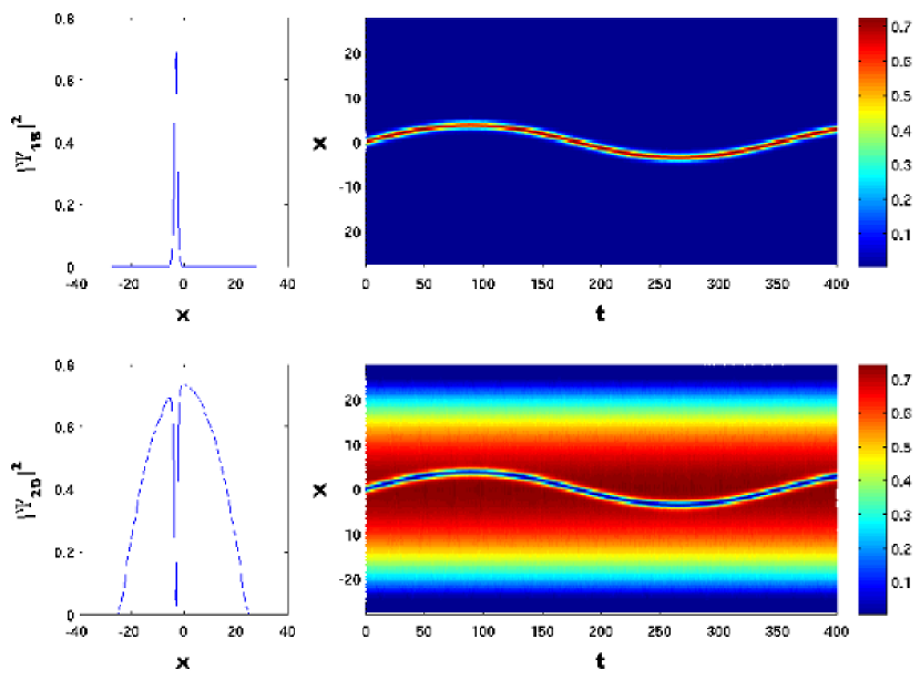
Figure 1: (Color online) Evolution of the bright-dark solitons of two-component BEC composed of two hyperfine states of the ⁸⁷Rb atom. Intraspecies scattering length $a_{12}=5.5$ nm ($b_{12}=13.6$) satisfying ratio formula (1) (top two panels), $a_{12}=5.4$ nm ($b_{12}=13.35$) disobeying the ratio formula (1) (bottom two panels). Other parameters $a_{11}=0.8\times 5.5$ nm ($b_{11}=10.88$), $a_{22}=1.2\times 5.5$ nm ($b_{22}=16.32$), $m_{1}=m_{2}=87$ au, $\omega_{1,\perp}=2\pi\times 710$ Hz, $\lambda_{1}=\lambda_{2}=0.2$, $v=0.04$, $N_{1}=500$, $N_{2}=6600$. The snapshots are depicting the soliton pairs at $t=20$ and $t=200$, respectively.

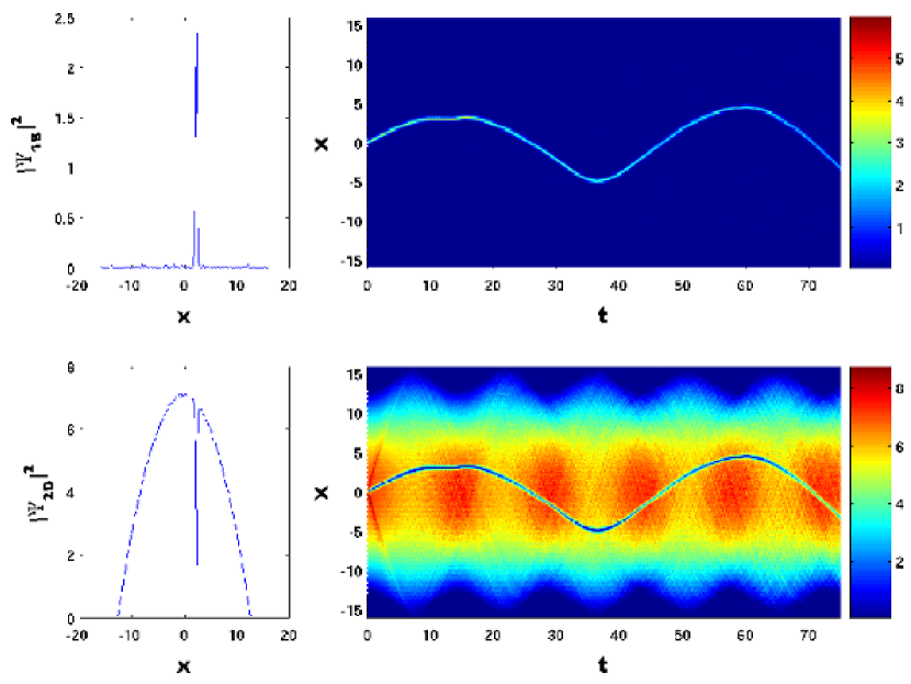
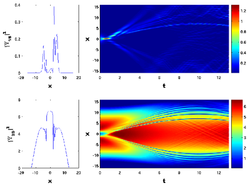
Figure 2: (Color online) Evolution of a bright-dark soliton pair in a two-component BEC composed of ²³Na and ⁸⁷Rb atoms. Intraspecies scattering length $a_{12}=6.831$ nm ($b_{12}=7.25$) satisfies formula (1) (top two panels), while $a_{12}=3.769$ nm ($b_{12}=4$) deviates from Eq. (1) (bottom two panels). Other parameters are: $a_{11}=2.7$ nm $(b_{11}=3.4)$, $a_{22}=5.5$ nm $(b_{22}=3.6)$, $m_{1}=23$ au, $m_{2}=87$ au, $\omega_{1,\perp}=2\pi\times 710$ Hz, $\lambda_{1}=\lambda_{2}=0.25$, $v=0.15$, $N_{1}=500$, $N_{2}=58000$. The snapshots are taken at $t=20$, and $t=2$, respectively.

In Fig. 1, we plotted a bright-dark soliton pair composed of two hyperfine states of ⁸⁷Rb atoms. The top two panels show the case when the inter-species interaction is chosen according to Eq. (1). Both solitons oscillate in the harmonic trap in a stable manner with an angular frequency slightly less than $\omega_{x}/\sqrt{2}$ what the one-dimensional Thomas-Fermi model predicts for a single dark soliton Busch and Anglin (2000). The difference is probably caused by the presence of the bright soliton, since the bright component fills the dip of the dark soliton, therefore the dark soliton has to drag this extra mass as well. This effect has recently been observed Becker et al. (2008) with a ⁸⁷Rb-⁸⁷Rb condensate, prepared in the $|F=2,m_{F}=0\rangle$ (bright soliton) and $|F=1,m_{F}=0\rangle$ (dark soliton) hyperfine states.

However, if $a_{12}$ (or equivalently $b_{12}$) is tuned away from this particular value, the stability is lost, and the initial forms of the solitons are destroyed by the destructive interference of the constantly emitted and re-captured sound waves. It is worthwhile to mention, although only as a qualitative statement, that the appearance of sound waves made the solitons’ oscillation faster (see the different range of time in the top two and bottom two panels of Fig. 1). The sound waves travel faster than the solitons, and after being reflected back from the edge of the condensate, they collide with the solitons. The subsequent collisions possibly speed up the oscillation and turn it into an irregular sloshing. Despite the irregular movement of the solitons, the dark component still captures the bright soliton during the motion.

In Fig. 2 the evolution of a bright-dark soliton pair in binary BEC composed of ²³Na and ⁸⁷Rb atoms is plotted with corresponding snapshots of the density distribution. Upper two panels exhibit the bright (²³Na) and dark (⁸⁷Rb) excitations, respectively, which are stable for a long period due to the fine tuning of scattering lengths $a_{ij}\,(i,j=1,2)$ which satisfy the P-test formula (1). On the lower two panels of Fig. 2 we see, however, that the initial soliton excitations do not remain stable but are rapidly dissolved due to detuning the interspecies scattering length $a_{12}$ from the value obeying the integrability condition expressed by Eq. (1).

Summarising, both examples exhibited in Figs. 1 and 2 show that a long lived stability of the bright-dark soliton pairs can be achieved only in case if the interatomic interaction parameters $a_{12}$ (or $b_{12}$) is chosen according to Eq. (1). This observation emphasises that there may be situations in the creation of two-component BECs when fine tuning of scattering lengths according to the P-test formula (1) may prove useful.

At the end of this section we briefly mention an early investigation of the stability of a heterogeneous two-component Bose-Einstein condensate by Law et al. Law et al. (1997). This work carried out a linear stability analysis by calculating the lowest eigenvalue of an excitation. In this approach the appearance of a negative eigenvalue signals instability. It was shown for a sodium-rubidium system, just as above, that stability occurs only in finite range of the inter-species scattering length. The direct quantitative comparison with our work, however, is less straightforward because Law et al.’s analysis assumes a spherically symmetric condensate, while we analyse a quasi one-dimensional model.

III.2 Static bright-bright soliton pairs

Let us now investigate the temporal stability of a static ($v=0$) bright-bright soliton pair obtained as the exact solution of Eqs. (5a-b) in the absence of a trapping potential ($\lambda_{i}=0$). The solutions have the form as in Eq. (11) where $\varphi_{i}(x)$ are chosen to have the functional forms given in Eqs. (18a-b).

The existence conditions (19) prescribe the relations between domains of the inter- and intra-species coupling strengths, $b_{ij}$, which are listed in Table 2. Moreover, the common wave-vector is $k=1/(2C_{1})$.

Case	$b_{11}$	$b_{22}$	Constraint on $b_{12}$
1	$+$	$-$	$b_{12}<b_{22}/\kappa$
2	$-$	$+$	$b_{12}<b_{11}/\kappa$
3a	$-$	$-$	$b_{22}/\kappa<b_{12}<\sqrt{b_{11}b_{22}}$	if $\kappa^{2}b_{11}<b_{22}$
3b			$b_{12}<b_{11}\kappa$	if $\kappa^{2}b_{11}<b_{22}$
3c			$b_{11}\kappa<b_{12}<\sqrt{b_{11}b_{22}}$	if $\kappa^{2}b_{11}>b_{22}$
3d			$b_{12}<b_{22}/\kappa$	if $\kappa^{2}b_{11}>b_{22}$
4	$+$	$+$	$b_{12}<-\sqrt{b_{11}b_{22}}$

Table 2: Various domains of inter- and intra-atomic interaction strengths, $b_{ij}$, permitting the existence of a bright-bright soliton pair.

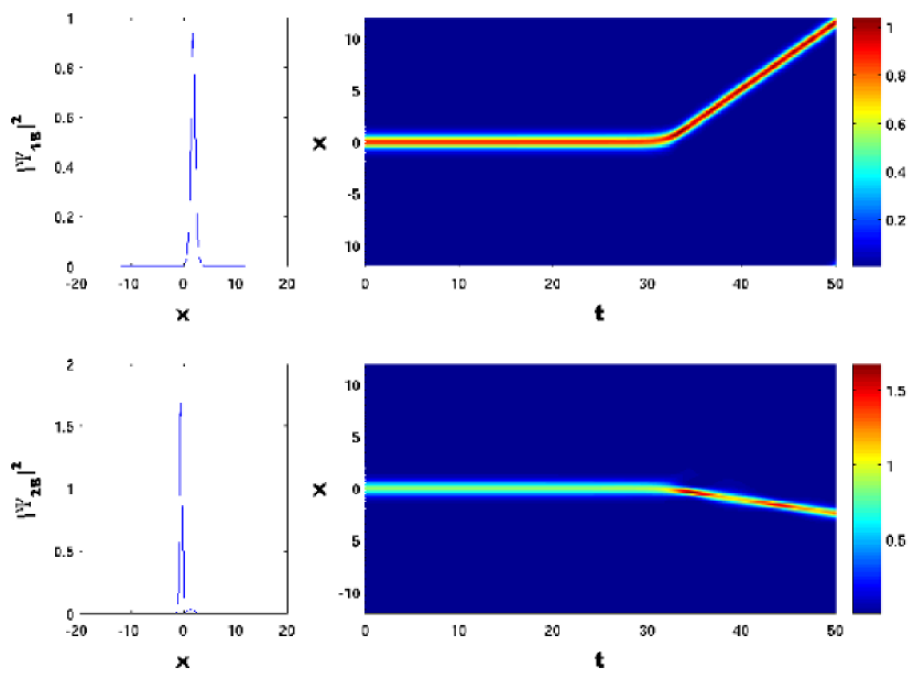
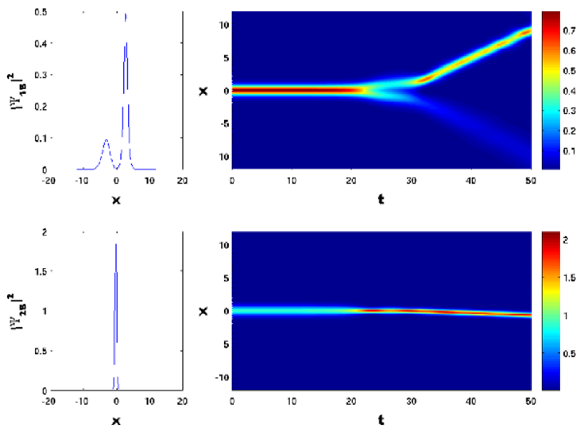
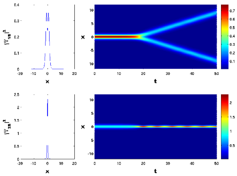
Figure 3: (Color online) Evolution of a bright-bright soliton pair in a binary BEC composed of ⁷Li and ³⁹K atoms. Intraspecies scattering lengths and atom numbers are $a_{12}=0.2$ nm ($b_{12}=0.46$), $N_{2}=2029$ (first two panels), $a_{12}=0.275$ nm ($b_{12}=0.64$) $N_{2}=2270$ (second pair of the panels), $a_{12}=0.3$ nm ($b_{12}=0.7$) $N_{2}=2347$ (third pair of the panels). Other parameters are: $a_{11}=-1.4$ nm $(b_{11}=-3.93)$, $a_{22}=-0.9$ nm $(b_{22}=-1.07)$, $m_{1}=7$ au, $m_{2}=39$ au, $\omega_{1,\perp}=2\pi\times 710$ Hz, $\lambda_{1}=\lambda_{2}=0$, $v=0$, $N_{1}=2000$. The snapshots are taken at $t=35$, $t=35$, and $t=20$, respectively.

Scenario 4, for example, describes two condensates for which the intra-species interactions are repulsive. This situation, using Hartree-Fock calculation, has been theoretically analysed Esry et al. (1997) soon after the observation of overlapping condensates prepared from two hyperfine states of ⁸⁷Rb Myatt et al. (1997). For this case, i.e. $m_{1}=m_{2}$, it was established that the two condensates cannot co-exist if $\left|a_{12}\right|<\sqrt{a_{11}a_{22}}$. Our approach reproduces and extends this result for the case of different species. This surprisingly simple relation can be understood using energetic arguments; if $b_{12}$ overcomes the geometric mean of the intra-species interaction strengths, the repulsion between the two condensates will separate the two condensate completely and they will not overlap any more. However, if the two species attract each other enough, i.e. $b_{12}<-\sqrt{b_{11}b_{22}}$, the attraction will dominate and can counteract the individual repulsion present in each component.

Another interesting scenario here is the one listed under the case 3a in Table 2 showing that it is possible to create a bright-bright pair, within the range $0<b_{12}<\sqrt{b_{11}b_{22}}$, in spite of the repulsive inter-atomic interaction. In order to investigate the stability of the bright-bright soliton pair in this domain we simulate the temporal evolution of the BEC system composed of ⁷Li and ³⁹K atoms accessible for experiments. As Fig. 3 shows, depending on the value of the interspecies interaction, two types of instability may occur. At values of $a_{12}$ less than a critical value of about $0.275$ nm, the two standing solitons begin to repel each other (first two panels) and depart from each other as they were particles, preserving the total zero momentum. Above the critical $a_{12}$ value the soliton with constituents of the smaller mass splits into two equal parts and the heavier component becomes a breather keeping its original place (third pair of panels). At the critical value of $a_{12}$ both types of instability can be observed (third and fourth panel) simultaneously.

Similar instability effects of a bright-bright and other soliton pairs have also been observed in Ref. Belmonte-Beitia et al. . The instability is explained by Kevrekidis at al. Kevrekidis et al. (2005) as the appearance of a negative eigenvalue pair obtained by a linear stability analysis. It has also been shown that higher order bright-bright soliton pairs would exhibit instability irrespectively of the system parameters. Interestingly, it is possible for one of the higher-order bright solitons, i.e., for the one which has the stronger self-attraction, to recover its stability by collapsing into one bright soliton and expel the other component from its original position.

Finally, it is important to note here, that the phases of the divided solitons are equal, therefore these particle-like wave-packets remain coherent with each other. Similarly to an optical beam splitter where light is divided into two coherent beams, one could divide these matter waves and use one of them as a probe and the other one as a control packet. The probe packet could undergo transformations, while the control packet is left to evolve freely, thereby a phase-difference could build up between the two packets. If the two packets are brought together again, the phase-difference could cause interference pattern which allows one to quantify coherence. This may potentially be helpful for calibrational purposes as well.

III.3 Dark-dark soliton pairs

At the end we are examining the third possible combination of soliton pairs; a dark soliton is excited in each condensate. Interestingly this pairing can be stable even if the interaction inside each condensate is attractive ($a_{11}$, $a_{22}<0$). The dark-dark solitons are described by the following formulas

$$\widetilde{\psi}_{1}^{\mathrm{DD}} = \left[i\sqrt{-C_{1}}\,v+\Phi^{\mathrm{TF}}_{1}(0)\varphi_{1}^{\mathrm{DD}}(x-vt)\right]\,\exp{\left(-i{\widetilde{E}}_{1}^{\mathrm{DD}}t\right)}\exp{\left[-i\left(\frac{b_{12}C_{2}}{\kappa^{2}}-b_{11}C_{1}\right)v^{2}t\right]},$$ (23a)

$$\widetilde{\psi}_{2}^{\mathrm{DD}} = \left[i\frac{\sqrt{C_{2}}}{\kappa}\,v+\Phi^{\mathrm{TF}}_{2}(0)\varphi_{2}^{\mathrm{DD}}(x-vt)\right]\,\exp{\left(-i{\widetilde{E}}_{2}^{\mathrm{DD}}t\right)}\exp{\left[-i\left(\frac{b_{22}C_{2}}{\kappa^{2}}-b_{12}C_{1}\right)v^{2}t\right]}.$$ (23b)

For our numerical investigations a ⁸⁷Rb–⁸⁷Rb system has been chosen, with repulsive intra-species interactions, $a_{11}=5.335$ nm and $a_{22}=5.665$ nm taken from Hall et al. (1998). This choice of coupling corresponds to scenario 4 of Table 3. Tuning $a_{12}$ into the positive regime results in a stable dark-dark soliton pairs, see top two panels of Fig. 4. In the bright-bright case we have found that if the intra-species interactions are attractive and the inter-species interactions are repulsive, the solutions are unstable. We have tested numerically that this observation is valid in the dark-dark case as well, if the sign of the interactions is inverted. Furthermore, our numerical calculation provided an interesting phenomenon in the dynamics of these solitons. Preparing the dark solitons in the same way as before (i.e., by superimposing onto the ground state) but reversing the sign of $a_{12}$, resulted not only in losing the long-term stability, but also in the decay of a dark soliton in one of the components, and emerging as a secondary dark soliton in the other component (bottom two panels of Fig. 4).

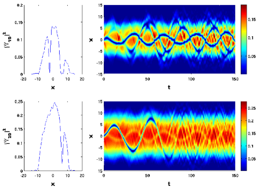
Figure 4: (Color online) Evolution of a dark-dark soliton pair in a binary BEC composed of ⁸⁷Rb and ⁸⁷Rb atoms. Intraspecies scattering lengths are $a_{12}=1.5$ nm ($b_{12}=3.62$) (top panel), $a_{12}=-1.5$ nm ($b_{12}=-3.62$) (bottom panel). Other parameters are: $a_{11}=0.97\times 5.5$ nm $(b_{11}=13.04)$, $a_{22}=1.03\times 5.5$ nm $(b_{22}=13.52)$, $m_{1}=87$ au, $m_{2}=87$ au, $\omega_{1,\perp}=2\pi\times 710$ Hz, $\lambda_{1}=\lambda_{2}=0.2$, $v=0.2$, $N_{1}=500$, $N_{2}=1600$. The snapshots are taken at $t=50$.

Case	$b_{11}$	$b_{22}$	Constraint on $b_{12}$
1	$+$	$-$	$b_{12}>b_{11}\kappa$
2	$-$	$+$	$b_{12}>b_{22}/\kappa$
3	$-$	$-$	$b_{12}>\sqrt{b_{11}b_{22}}$
4a	$+$	$+$	$-\sqrt{b_{11}b_{22}}<b_{12}<b_{22}/\kappa$	if $\kappa^{2}b_{11}>b_{22}$
4b			$b_{12}>b_{11}\kappa$	if $\kappa^{2}b_{11}>b_{22}$
4c			$-\sqrt{b_{11}b_{22}}<b_{12}<b_{11}\kappa$	if $\kappa^{2}b_{11}<b_{22}$
4d			$b_{12}>b_{22}/\kappa$	if $\kappa^{2}b_{11}<b_{22}$

Table 3: Various domains of inter- and intra-atomic interaction strengths, $b_{ij}$, permitting the existence of a dark-dark soliton pair.

IV Summary

We have considered the existence and stability of soliton excitations in a two-component Bose-Einstein condensate both analytically and numerically. Our model allows the components to represent different elements ($m_{1}\neq m_{2}$), but we also included those cases when two hyperfine states of the same element constitute the condensates. We excluded the possibility that these components can transmute into each other, i.e. the hyperfine states cannot be driven into each other. The dynamics of these condensates, within the mean-field zero-temperature approximation, are governed by the coupled Gross-Pitaevskii equations. We chose our presentation to be suitable for combining analytical results with earlier numerical investigations, e.g. Schumayer and Apagyi (2001); Xun-Xu et al. (2010); Liu et al. (2009).

The occurrence of particle-like excitations together with conserved quantities are associated with the integrability of a nonlinear evolution field-equation, such as the coupled Gross-Pitaevskii equations. Using the results of a recent Painlevé analysis of the coupled Gross-Pitaevskii equation Schumayer and Apagyi (2001), we showed how the system parameters determine the integrability of this system. However, for the CGP equations the studies so far restricted themselves for either equal coupling coefficients ($b_{11}=b_{12}=b_{22}$) and/or equal masses. We note here that excitations with long lifetime may exist for a nonlinear evolution equation even when the integrability conditions are violated Novoa et al. (2008), but these cases are possibly exceptional and do not represent the generic behaviour.

We examined those ranges of system parameters which permit coupled soliton solutions of the governing equations (5a-b). Here, we utilised the two well-known one-soliton solutions of the one-component nonlinear Schrödinger equation; the bright and dark solitons. These excitations then spatially modify the Thomas-Fermi ground state in our theoretical description or by the appropriate ground state in our numerical simulation. We found analytically that each possible pair of these solitons have a range of system parameters where they are stable, and presented these ranges in tabulated form in Tabs. 1, 2, and 3. One can present these findings differently, if the intra-species coupling coefficients are held relatively fixed, and only the inter-species one is tuned. For example, if we assume $b_{11}$ and $b_{22}$ to be positive (effective repulsive interaction) then the three tables 1, 2, and 3 can be combined into one graph (see Fig. 5).

Figure 5: Ranges of the inter-species coupling coefficient, $b_{12}$, in which different types of soliton pairs can exist and are stable. The top graph is valid if $\kappa^{2}b_{11}<b_{22}$, while the lower graph is for the complementary case, i.e. $\kappa^{2}b_{11}>b_{22}$. The dotted line shows the result of the Painlevé-test (1) in the case of harmonic trapping potentials.

Moreover, we also examined how the stability of these soliton pairs is changing if the inter-species coupling coefficient is detuned from the value predicted by the Painleé-analysis via Eq. (1). It was shown, irrespectively of the pairing, that the stability is lost, although the pairs were not equally sensitive to the detuning, e.g. the motion of the bright-dark pair became erratic and preserved its periodicity only qualitatively after changing $a_{12}$ from 5.5 nm to 5.4 nm.

Two types of instability of static bright-bright soliton pairs composed of species with unequal masses have been observed. When the interspecies interaction lies below a critical value ($0<b_{12}<b_{12}^{\mathrm{cr}}$), the static bright-bright pair evolves into a repulsive, momentum conserving, moving soliton pair. When the value of $b_{12}>b_{12}^{cr}$ then one of the bright soliton (the constituent with smaller mass) splits into two equal portion of same phase while the other bright soliton becomes a breather.

Well below the critical temperature of the Bose-Einstein condensate our description is expected to be adequate and the results could help experimentalist to modify the scattering lengths via Feshbach resonance into a range where stable soliton pairs exist. As the temperature increases, however, the interaction with the thermal cloud becomes more and more important, and could not be neglected any more. We have not yet examined how the interplay between the condensates and the thermal clouds (for each component) would modify the dynamics. This needs further research beyond the mean field description.

Acknowledgment — D. Schumayer acknowledges financial support from NERF-UOOX0703 (NZ) and also by the University of Otago. G. Csire and B. Apagyi thank DFG for subsidising their stay at Institute of Theoretical Physics, University of Giessen.

References

- Bloch et al. (2008) I. Bloch, J. Dalibard, and W. Zwerger, Rev. Mod. Phys., 80, 885 (2008).
- Myatt et al. (1997) C. J. Myatt, E. A. Burt, R. W. Ghrist, E. A. Cornell, and C. E. Wieman, Phys. Rev. Lett., 78, 586 (1997).
- Stamper-Kurn et al. (1998) D. M. Stamper-Kurn, M. R. Andrews, A. P. Chikkatur, S. Inouye, H.-J. Miesner, J. Stenger, and W. Ketterle, Phys. Rev. Lett., 80, 2027 (1998).
- Modugno et al. (2001) G. Modugno, G. Ferrari, G. Roati, R. J. Brecha, A. Simoni, and M. Inguscio, Science, 294, 1320 (2001).
- Thalhammer et al. (2008) G. Thalhammer, G. Barontini, L. D. Sarlo, J. Catani, F. Minardi, and M. Inguscio, Phys. Rev. Lett., 100, 210402 (2008).
- Mudrich et al. (2002) M. Mudrich, S. Kraft, K. Singer, R. Grimm, A. Mosk, and M. Weidemüller, Phys. Rev. Lett., 88, 253001 (2002).
- Pilch et al. (2009) K. Pilch, A. D. Lange, A. Prantner, G. Kerner, F. Ferlaino, H.-C. Nägerl, and R. Grimm, Phys. Rev. A, 79, 042718 (2009).
- Papp et al. (2008) S. B. Papp, J. M. Pino, and C. E. Wieman, Phys. Rev. Lett., 101, 040402 (2008).
- Schumayer and Apagyi (2002) D. Schumayer and B. Apagyi, Phys. Rev. A, 65, 053614 (2002).
- Hasegawa and Matsumoto (2002) A. Hasegawa and M. Matsumoto, Optical Solitons in Fibers, 3rd ed. (Springer, 2002).
- Burger et al. (1999) S. Burger, K. Bongs, S. Dettmer, W. Ertmer, K. Sengstock, A. Sanpera, G. V. Shlyapnikov, and M. Lewenstein, Phys. Rev. Lett., 83, 5198 (1999).
- Denschlag et al. (2000) J. Denschlag, J. E. Simsarian, D. L. Feder, C. W. Clark, L. A. Collins, J. Cubizolles, L. Deng, E. W. Hagley, K. Helmerson, W. P. Reinhardt, S. L. Rolston, B. I. Schneider, and W. D. Phillips, Science, 287, 97 (2000).
- Khaykovich et al. (2002) L. Khaykovich, F. Schreck, G. Ferrari, T. Bourdel, J. Cubizolles, L. D. Carr, Y. Castin, and C. Salomon, Science, 296, 1290 (2002).
- Strecker et al. (2002) K. E. Strecker, G. B. Partridge, A. G. Truscott, and R. G. Hulet, Nature, 417, 150 (2002), ISSN 0028-0836.
- Öhberg and Santos (2001) P. Öhberg and L. Santos, Phys. Rev. Lett., 86, 2918 (2001).
- Liu and Hao (2002) J. Liu and Z. Hao, Phys. Rev. E, 65, 066601 (2002).
- Busch and Anglin (2001) T. Busch and J. R. Anglin, Phys. Rev. Lett., 87, 010401 (2001).
- Becker et al. (2008) C. Becker, S. Stellmer, P. Soltan-Panahi, S. Dorscher, M. Baumert, E.-M. Richter, J. Kronjager, K. Bongs, and K. Sengstock, Nature Physics, 4, 496 (2008), ISSN 1745-2473.
- Ginsberg et al. (2005) N. S. Ginsberg, J. Brand, and L. V. Hau, Phys. Rev. Lett., 94, 040403 (2005).
- Steeb et al. (1984) W.-H. Steeb, M. Kloke, and B.-M. Spieker, J. Phys. A, 17, L825 (1984), ISSN 0305-4470.
- Zakharov and Shabat (1972) V. E. Zakharov and A. B. Shabat, Sov. Phys. JETP, 34, 62 (1972).
- Zakharov and Manakov (1974) V. E. Zakharov and S. V. Manakov, Theoretical and Mathematical Physics, 19, 551 (1974).
- Zakharov and Manakov (1985) V. E. Zakharov and S. V. Manakov, Functional Analysis and Its Applications, 19, 89 (1985).
- Sahadevan et al. (1986) R. Sahadevan, K. M. Tamizhmani, and M. Lakshmanan, J. Phys. A, 19, 1783 (1986), ISSN 0305-4470.
- Clarkson (1988) P. Clarkson, Proc. Roy. Soc. Edinb. A, 109, 109 (1988).
- Schumayer and Apagyi (2001) D. Schumayer and B. Apagyi, J. Phys. A, 34, 4969 (2001).
- Brazhnyi et al. (2009) V. A. Brazhnyi, V. V. Konotop, V. M. Perez-Garcia, and H. Ott, Phys. Rev. Lett., 102, 144101 (2009).
- Rajendran et al. (2009) S. Rajendran, P. Muruganandam, and M. Lakshmanan, J. Phys. B, 42, 145307 (2009).
- Nakkeeran (2001) K. Nakkeeran, J. Phys. A, 34, 5111 (2001), ISSN 0305-4470.
- Gross (1961) E. Gross, Il Nuovo Cimento, 20, 454 (1961).
- Pitaevskii (1961) L. P. Pitaevskii, Soviet Phys.– JETP, 13, 451 (1961).
- Liu et al. (2009) X. Liu, H. Pu, B. Xiong, W. M. Liu, and J. Gong, Phys. Rev. A, 79, 013423 (2009).
- Schumayer and Apagyi (2004) D. Schumayer and B. Apagyi, Phys. Rev. A, 69, 043620 (2004).
- Javanainen and Ruostekoski (2006) J. Javanainen and J. Ruostekoski, J. Phys. A, 39, L179 (2006).
- Lehtovaara et al. (2007) L. Lehtovaara, J. Toivanen, and J. Eloranta, J. Comp. Phys., 221, 148 (2007), ISSN 0021-9991.
- Busch and Anglin (2000) T. Busch and J. R. Anglin, Phys. Rev. Lett., 84, 2298 (2000).
- Law et al. (1997) C. K. Law, H. Pu, N. P. Bigelow, and J. H. Eberly, Phys. Rev. Lett., 79, 3105 (1997).
- Esry et al. (1997) B. D. Esry, C. H. Greene, J. J. P. Burke, and J. L. Bohn, Phys. Rev. Lett., 78, 3594 (1997).
- (39) J. Belmonte-Beitia, V. M. Perez-Garcia, and V. Brazhnyi, Communications in Nonlinear Science and Numerical Simulation, In Press, Corrected Proof, , ISSN 1007-5704.
- Kevrekidis et al. (2005) P. G. Kevrekidis, H. Susanto, R. Carretero-González, B. A. Malomed, and D. J. Frantzeskakis, Phys. Rev. E, 72, 066604 (2005).
- Hall et al. (1998) D. S. Hall, M. R. Matthews, J. R. Ensher, C. E. Wieman, and E. A. Cornell, Phys. Rev. Lett., 81, 1539 (1998).
- Xun-Xu et al. (2010) L. Xun-Xu, Z. Xiao-Fei, and Z. Peng, Chinese Physics Letters, 27, 070306 (2010).
- Novoa et al. (2008) D. Novoa, B. A. Malomed, H. Michinel, and V. M. Perez-Garcia, Phys. Rev. Lett., 101, 144101 (2008).