Generalized Eigenvalue Problems with Specified Eigenvalues

Abstract

We consider the distance from a (square or rectangular) matrix pencil to the nearest matrix pencil in 2-norm that has a set of specified eigenvalues. We derive a singular value optimization characterization for this problem and illustrate its usefulness for two applications. First, the characterization yields a singular value formula for determining the nearest pencil whose eigenvalues lie in a specified region in the complex plane. For instance, this enables the numerical computation of the nearest stable descriptor system in control theory. Second, the characterization partially solves the problem posed in [Boutry et al. 2005] regarding the distance from a general rectangular pencil to the nearest pencil with a complete set of eigenvalues. The involved singular value optimization problems are solved by means of BFGS and Lipschitz-based global optimization algorithms.

Key words. Matrix pencils, eigenvalues, optimization of singular values, inverse eigenvalue problems, Lipschitz continuity, Sylvester equation.

AMS subject classifications. 65F15, 65F18, 90C26, 90C56

1 Introduction

Consider a matrix pencil $A-\lambda B$ where $A,B\in{\mathbb{C}}^{n\times m}$ with $n\geq m$. Then a scalar $\rho\in{\mathbb{C}}$ is called an eigenvalue of the pencil if there exists a nonzero vector $v\in{\mathbb{C}}^{n}$ such that

$$(A-\rho B)v=0.$$ (1)

The vector $v$ is said to be a (right) eigenvector associated with $\rho$ and the pair $(\rho,v)$ is said to be an eigenpair of the pencil.

In the square case $m=n$, the eigenvalues are simply given by the roots of the characteristic polynomial $\det(A-\lambda B)$ and there are usually $n$ eigenvalues, counting multiplicities. The situation is quite the opposite for $n>m$. Generically, a rectangular pencil $A-\lambda B$ has no eigenvalues at all. To see this, notice that a necessary condition for the satisfaction of (1) is that $n!/\left((n-m)!m!\right)$ polynomials, each corresponding to the determinant of a pencil obtained by choosing $m$ rows of $A-\lambda B$ out of $n$ rows, must have a common root. Also, the generic Kronecker canonical form of a rectangular matrix pencil only consists of singular blocks (see [9]). Hence, (1) is an ill-posed problem and requires reformulation before admitting numerical treatment.

To motivate our reformulation of (1), we describe a typical situation giving rise to rectangular matrix pencils. Let $M\in\mathbb{C}^{n\times n}$ and suppose that the columns of $U\in\mathbb{C}^{n\times m}$ form an orthonormal basis for a subspace $\mathcal{W}\subset\mathbb{C}^{n}$ known to contain approximations to some eigenvectors of $M$. Then it is quite natural to consider the $n\times m$ matrix pencil

$$A-\lambda B:=MU-\lambda U.$$ (2)

The approximations contained in $\mathcal{W}$ and the approximate eigenpairs of $A-\lambda B$ are closely connected to each other. In one direction, suppose that $(\rho,x)$ with $x\in\mathcal{W}$ satisfies

$$(M+\Delta M-\rho I)x=0$$ (3)

for some (small) perturbation $\Delta M$. Then there is $v\in\mathbb{C}^{n}$ such that $x=Uv$. Moreover, we have

$$(A+\Delta A-\rho B)v=0$$ (4)

with $\Delta A:=\Delta M\cdot U$ satisfying $\|\Delta A\|_{2}\leq\|\Delta M\|_{2}$. In the other direction, the relation (4) with an arbitrary $\Delta A$ implies (3) with $\Delta M=\Delta A\cdot U^{\ast}$ satisfying $\|\Delta M\|_{2}=\|\Delta A\|_{2}$. Unless $M$ is normal, the first part of this equivalence between approximate eigenpairs of $M$ and $A-\lambda B$ does not hold when the latter is replaced by the more common compression $U^{\ast}MU$. This observation has led to the use of rectangular matrix pencils in, e.g., large-scale pseudospectra computation (see [31]) and Ritz vector extraction (see [17]).

This paper is concerned with determining the 2-norm distance from the pencil $A-\lambda B$ to the nearest pencil $(A+\Delta A)-\lambda B$ with a subset of specified eigenvalues. To be precise, let ${\mathbb{S}}=\{\lambda_{1},\dots,\lambda_{k}\}$ be a set of distinct complex numbers and let $r$ be a positive integer. Let $m_{j}(A+\Delta A,B)$ denote the (possibly zero) algebraic multiplicity of $\lambda_{j}$ as an eigenvalue of $(A+\Delta A)-\lambda B$. Then we consider the distance

$$\tau_{r}({\mathbb{S}}):=\inf\Big{\{}\|\Delta A\|_{2}:\sum_{j=1}^{k}m_{j}(A+\Delta A,B)\geq r\Big{\}}.$$ (5)

We allow $B$ to be rank-deficient. However, we require that ${\rm rank}(B)\geq r$. Otherwise, if ${\rm rank}(B)<r$, the pencil $(A+\Delta A)-\lambda B$ has fewer than $r$ finite eigenvalues for all $\Delta A$ and consequently the distance $\tau_{r}({\mathbb{S}})$ is ill-posed.

For $k=r=1$, it is relatively easy to see that

$$\tau_{1}(\{\lambda_{1}\})=\sigma_{m}(A-\lambda_{1}B),$$

where, here and in the following, $\sigma_{k}$ denotes the $k$th largest singular value of a matrix. (The particular form of this problem with $k=r=1$, and when $A$ and $B$ are perturbed simultaneously, is also studied for instance in [7].) One of the main contributions of this paper is a derivation of a similar singular value optimization characterization for general $k$ and $r$, which facilitates the computation of $\tau_{r}({\mathbb{S}})$. Very little seems to be known in this direction. Existing results concern the square matrix case ($m=n$ and $B=I$); see the works by [24] for $k=1$ and $r=2$ as well as [21] for $k=2$ and $r=2$, [15] for $k=1$ and $r=3$, and [25] for $k=1$ and arbitrary $r$. Some attempts have also been made by [22] for arbitrary $k$ and $r$ and for the square matrix case, and by [27] for $k=1$ and $r=2$ and for the square matrix polynomial case.

Another class of applications arises in (robust) control theory, where a number of tasks require the determination of a (minimal) perturbation that moves some or all eigenvalues into a certain region in the complex plane. With the region of interest denoted by $\Omega\subseteq\mathbb{C}$, the results in this paper are an important step towards rendering the numerical computation of the distance

$$\tau_{r}(\Omega) := \inf\big{\{}\|\Delta A\|_{2}:(A+\Delta A)-\lambda B\;\text{has $r$ finite eigenvalues in $\Omega$}\big{\}}$$

$$= \inf_{{\mathbb{S}}\subseteq\Omega}\tau_{r}({\mathbb{S}})$$

feasible. Here and in the following, multiple eigenvalues are counted according to their algebraic multiplicities. For $r=1$ and $\Omega$ equal to $\mathbb{C}^{+}$ (right-half complex plane), the quantity $\tau_{1}(\mathbb{C}^{+})$ amounts to the distance to instability, also called stability radius. In [32], a singular value characterization of $\tau_{1}(\mathbb{C}^{+})$ was provided, forming the basis of a number of algorithms for computing $\tau_{1}(\mathbb{C}^{+})$, see, e.g., [3, 6]. In our more general setting, we can also address the converse question: Given an unstable matrix pencil $A-\lambda B$, determine the closest stable pencil. Notice that this problem is intrinsically harder than the distance to instability. For the distance to instability it suffices to perturb the system so that one of the eigenvalues is in the undesired region. On the other hand to make an unstable system stable one needs to perturb the system so that all eigenvalues lie in the region of stability.

An important special case, $\Omega=\mathbb{C}$ leads to

$$\tau_{r}({\mathbb{C}}) := \inf\{\|\Delta A\|_{2}:(A+\Delta A)-\lambda B\;\;{\rm has}\;r\;{\rm finite}\;{\rm eigenvalues}\;\}$$

$$= \inf_{{\mathbb{S}}\subseteq{\mathbb{C}}}\tau_{r}({\mathbb{S}}).$$

For $r=1$ and particular choices of rectangular $A$ and $B$, the distance $\tau_{1}({\mathbb{C}})$ corresponds to the distance to uncontrollability for a matrix pair (see [5, 10]). For general $r$, a variant of this distance was suggested in [2] to solve an inverse signal processing problem approximately. More specifically, this problem is concerned with the identification of the shape of a region in the complex plane given the moments over the region. If the region is assumed to be a polygon, then its vertices can be posed as the eigenvalues of a rectangular pencil $A-\lambda B$, where $A$ and $B$ are not exact due to measurement errors, causing the pencil to have no eigenvalues (see [11] for details). Then the authors attempt to locate nearby pencils with a complete set of eigenvalues. In this work we allow perturbations to $A$ only, but not to $B$. This restriction is only justified if the absolute value of $\lambda$ does not become too small. We consider our results and technique as significant steps towards the complete solution of the problem posed in [11].

The outline of this paper is as follows. In the next section, we review the Kronecker canonical form for the pencil $A-\lambda B$. In §3, we derive a rank characterization for the condition $\sum_{j=1}^{k}m_{j}(A,B)\geq r$. This is a crucial prerequisite for deriving the singular value characterizations of $\tau_{r}({\mathbb{S}})$ in §4. We discuss several corollaries of the singular value characterizations for $\tau_{r}({\mathbb{S}})$, in particular for $\tau_{r}(\Omega)$ and $\tau_{r}({\mathbb{C}})$, in §5. The singular value characterizations are deduced under certain mild multiplicity and linear independence assumptions. Although we expect these assumptions to be satisfied for examples of practical interest, they may fail to hold as demonstrated by an academic example in §6. Interestingly, the singular value characterization remains true for this example despite the fact that our derivation no longer applies. Finally, a numerical approach to solving the involved singular value optimization problems is briefly outlined in §7 and applied to a number of settings in §8. The main point of the developed numerical method and the experiments is to demonstrate that the singular value characterizations facilitate the computation of $\tau_{r}({\mathbb{S}})$, $\tau_{r}(\Omega)$ and $\tau_{r}({\mathbb{C}})$. We do not claim that the method outlined here is as efficient as it could be, neither do we claim that it is reliable.

2 Kronecker Canonical Form

Given a matrix pencil $A-\lambda B\in{\mathbb{C}}^{n\times m}$, the Kronecker canonical form (KCF), see [13], states the existence of invertible matrices $P\in{\mathbb{C}}^{n\times n}$ and $Q\in{\mathbb{C}}^{m\times m}$ such that the transformed pencil $P(A-\lambda B)Q$ is block diagonal with each diagonal block taking the form

$$J_{p}(\alpha)-\lambda I_{p}\quad\text{or}\quad I_{p}-\lambda J_{p}(0)\quad\text{or}\quad F_{p}-\lambda G_{p}\quad\text{or}\quad F_{p}^{T}-\lambda G_{p}^{T},$$

where

$$J_{p}(\alpha)=\underbrace{\left[\begin{array}[]{cccc}\alpha&1\\[-5.0pt] &\alpha&\ddots\\[-5.0pt] &&\ddots&1\\ &&&\alpha\end{array}\right]}_{p\times p},\ F_{p}=\underbrace{\left[\begin{array}[]{cccc}1&0\\ &\ddots&\ddots\\ &&1&0\end{array}\right]}_{p\times(p+1)},\ G_{p}=\underbrace{\left[\begin{array}[]{cccc}0&1\\ &\ddots&\ddots\\ &&0&1\end{array}\right]}_{p\times(p+1)}$$ (6)

for some $\alpha\in{\mathbb{C}}$. Regular blocks take the form $J_{p}(\alpha)-\lambda I_{p}$ or $I_{p}-\lambda J_{p}(0)$, with $p\geq 1$, corresponding to finite or infinite eigenvalues, respectively. The blocks $F_{p}-\lambda G_{p}$ and $F_{p}^{T}-\lambda G_{p}^{T}$ are called right and left singular blocks, respectively, with $p\geq 0$ corresponding to a so called Kronecker index.

In large parts of this paper, indeed until the main singular value optimization characterization, we will assume that $A-\lambda B$ has no right singular blocks $F_{p}-\lambda G_{p}$. Eventually, we will remove this assumption by treating the occurence of such blocks separately in Section 4.3.

3 Rank Characterization for Pencils with Specified Eigenvalues

In this section we derive a rank characterization for the satisfaction of the condition

$$\sum_{j=1}^{k}m_{j}(A,B)\geq r,$$ (7)

where $m_{j}(A,B)$ denotes the algebraic multiplicity of the eigenvalue $\lambda_{j}$. The following classical result [13, Theorem 1, p. 219] concerning the dimension of the solution space for a Sylvester equation will play a central role.

Theorem 3.1.

Let $F\in{\mathbb{C}}^{m\times m}$ and $G\in{\mathbb{C}}^{r\times r}$. Then the dimension of the solution space for the Sylvester equation

$$FX-XG=0$$

only depends on the Jordan canonical forms of the matrices $F$ and $G$. Specifically, suppose that $\mu_{1},\dots,\mu_{\ell}$ are the common eigenvalues of $F$ and $G$. Let $c_{j,1},\dots,c_{j,\ell_{j}}$ and $p_{j,1},\dots,p_{j,\tilde{\ell}_{j}}$ denote the sizes of the Jordan blocks of $F$ and $G$ associated with the eigenvalue $\mu_{j}$, respectively. Then

$${\rm dim}\{X\in{\mathbb{C}}^{m\times r}:FX-XG=0\}=\sum_{j=1}^{\ell}\sum_{i=1}^{\ell_{j}}\sum_{q=1}^{\tilde{\ell}_{j}}\min(c_{j,i},p_{j,q}).$$

For our purposes, we need to extend the result of Theorem 3.1 to a generalized Sylvester equation of the form

$$AX-BXC=0,$$ (8)

where $C$ is a matrix with the desired set of eigenvalues ${\mathbb{S}}$ and with correct algebraic multiplicities. For this type of generalized Sylvester equation, the extension is straightforward. To see this, let us partition the KCF

$$P(A-\lambda B)Q={\rm diag}\left(A_{F}-\lambda I,I-\lambda A_{I},A_{S}-\lambda B_{S}\right),$$ (9)

such that

• $A_{F}-\lambda I$ contains all regular blocks corresponding to finite eigenvalues;

• $I-\lambda A_{I}$ contains all regular blocks corresponding to infinite eigenvalues;

• $A_{S}-\lambda B_{S}$ contains all left singular blocks of the form $F_{p}^{T}-\lambda G_{p}^{T}$.

As explained in Section 2, we exclude the occurence of right singular blocks for the moment. Note that the finite eigenvalues of $A-\lambda B$ are equal to the eigenvalues of $A_{F}$ with the same algebraic and geometric multiplicities.

Using (9), $X$ is a solution of the generalized Sylvester equation (8) if and only if

$$(PAQ)(Q^{-1}X)-(PBQ)(Q^{-1}X)C=0\;\;\;\Longleftrightarrow\;\;\;{\rm diag}\left(A_{F},I,A_{S}\right)Y-{\rm diag}\left(I,A_{I},B_{S}\right)YC=0$$

where $Y=Q^{-1}X$. Consequently, the dimension of the solution space for (8) is the sum of the solution space dimensions of the equations

$$A_{F}Y_{1}-Y_{1}C=0\;\;\;\;{\rm and}\;\;\;\;Y_{2}-A_{I}Y_{2}C=0\;\;\;\;{\rm and}\;\;\;\;A_{S}Y_{3}-B_{S}Y_{3}C=0.$$

Results by [9] show that the last two equations only admit the trivial solutions $Y_{2}=0$ and $Y_{3}=0$. To summarize: the solution spaces of the generalized Sylvester equation (8) and the (standard) Sylvester equation

$$A_{F}X-XC=0$$

have the same dimension. Applying Theorem 3.1 we therefore obtain the following result.

Theorem 3.2.

Let $A,B\in{\mathbb{C}}^{n\times m}$ with $n\geq m$ be such that the KCF of $A-\lambda B$ does not contain right singular blocks. Then the dimension of the solution space for the generalized Sylvester equation

$$AX-BXC=0$$

only depends on the Kronecker canonical form of $A-\lambda B$ and the Jordan canonical form of $C\in{\mathbb{C}}^{r\times r}$. Specifically suppose that $\mu_{1},\dots,\mu_{\ell}$ are the common eigenvalues of $A-\lambda B$ and $C$. Let $c_{j,1},\dots,c_{j,\ell_{j}}$ and $p_{j,1},\dots,p_{j,\tilde{\ell}_{j}}$ denote the sizes of the Jordan blocks of $A-\lambda B$ and $C$ associated with the eigenvalue $\mu_{j}$, respectively. Then

$${\rm dim}\{X\in{\mathbb{C}}^{m\times r}:AX-BXC=0\}=\sum_{j=1}^{\ell}\sum_{i=1}^{\ell_{j}}\sum_{q=1}^{\tilde{\ell}_{j}}\min(c_{j,i},p_{j,q}).$$

We now apply the result of Theorem 3.2 to the generalized Sylvester equation

$$AX-BXC(\mu,\Gamma)=0,$$ (10)

where $C(\mu,\Gamma)$ takes the form

$$C(\mu,\Gamma)=\left[\begin{array}[]{cccc}\mu_{1}&-\gamma_{21}&\dots&-\gamma_{r1}\\ 0&\mu_{2}&\ddots&\vdots\\[-2.84544pt] &&\ddots&-\gamma_{r,r-1}\\ 0&&&\mu_{r}\\ \end{array}\right],$$ (11)

with

$$\mu=\left[\begin{array}[]{cccc}\mu_{1}&\mu_{2}&\dots&\mu_{r}\end{array}\right]^{T}\in{\mathbb{S}}^{r},\quad\Gamma=\left[\begin{array}[]{cccc}\gamma_{21}&\gamma_{31}&\dots&\gamma_{r,r-1}\end{array}\right]^{T}\in{\mathbb{C}}^{r(r-1)/2}.$$

As explained in the introduction, the set ${\mathbb{S}}=\{\lambda_{1},\dots,\lambda_{k}\}$ contains the desired approximate eigenvalues. Suppose that $\lambda_{j}$ occurs $p_{j}$ times in $\mu$. Furthermore, as in Theorem 3.2, denote the sizes of the Jordan blocks of $A-\lambda B$ and $C(\mu,\Gamma)$ associated with the scalar $\lambda_{j}$ by $c_{j,1},\dots,c_{j,\ell_{j}}$ and $p_{j,1},\dots,p_{j,\tilde{\ell}_{j}}$, respectively. Note that $p_{j}=\sum_{q=1}^{\tilde{\ell}_{j}}p_{j,q}$. In fact, for generic values of $\Gamma$ the matrix $C(\mu,\Gamma)$ has at most one Jordan block of size $p_{j}$ associated with $\lambda_{j}$ for $j=1,\dots,k$, see [9]. In the following, we denote this set of generic values for $\Gamma$ by ${\mathcal{G}}(\mu)$. By definition, this set depends on $\mu$ but not on $A-\lambda B$.

First, suppose that inequality (7) holds. If we choose $\mu$ such that $\sum_{j=1}^{k}p_{j}=r$ and $p_{j}\leq m_{j}(A,B)=\sum_{i=1}^{\ell_{j}}c_{j,i}$, then Theorem 3.2 implies that the dimension of the solution space for the generalized Sylvester equation (10) is

$$\sum_{j=1}^{k}\sum_{i=1}^{\ell_{j}}\sum_{q=1}^{\tilde{\ell}_{j}}\min(c_{j,i},p_{j,q})\geq\sum_{j=1}^{k}\sum_{i=1}^{\ell_{j}}\min(c_{j,i},p_{j})\geq\sum_{j=1}^{k}\min(m_{j}(A,B),p_{j})=\sum_{j=1}^{k}p_{j}=r.$$

In other words, there exists a vector $\mu$ with components from $\mathbb{S}$ such that the dimension of the solution space of the Sylvester equation (10) is at least $r$.

Now, on the contrary, suppose that inequality (7) does not hold. Then for generic values $\Gamma\in{\mathcal{G}}(\mu)$, the solution space dimension of (10) is

$$\sum_{j=1}^{k}\sum_{i=1}^{\ell_{j}}\min(c_{j,i},p_{j})\leq\sum_{j=1}^{k}\sum_{i=1}^{\ell_{j}}c_{j,i}=\sum_{j=1}^{k}m_{j}(A,B)<r.$$

In other words, no matter how $\mu$ is formed from $\mathbb{S}$, the dimension is always less than $r$ for $\Gamma\in{\mathcal{G}}(\mu)$. This shows the following result.

Theorem 3.3.

Let $A,B\in{\mathbb{C}}^{n\times m}$ with $n\geq m$ be such that the KCF of $A-\lambda B$ does not contain right singular blocks. Consider a set ${\mathbb{S}}=\{\lambda_{1},\dots,\lambda_{k}\}$ of distinct complex scalars, and a positive integer $r$. Then the following two statements are equivalent.

1. $\sum_{j=1}^{k}m_{j}(A,B)\geq r$, where $m_{j}(A,B)$ is the algebraic multiplicity of $\lambda_{j}$ as an eigenvalue of $A-\lambda B$.

2. There exists $\mu\in{\mathbb{S}}^{r}$ such that

   $${\rm dim}\{X\in{\mathbb{C}}^{m\times r}:AX-BXC(\mu,\Gamma)=0\}\geq r$$

   for all $\Gamma\in{\mathcal{G}}(\mu)$, where $C(\mu,\Gamma)$ is defined as in (11).

To obtain a matrix formulation of Theorem 3.3, we use the Kronecker product $\otimes$ to vectorize the generalized Sylvester equation (10) and obtain

$$\left(((I\otimes A)-(C^{T}(\mu,\Gamma)\otimes B)\right){\rm vec}(X)={\mathcal{L}}(\mu,\Gamma,A,B){\rm vec}(X)=0,$$

with the lower block triangular matrix

$${\mathcal{L}}(\mu,\Gamma,A,B):=\left[\begin{array}[]{ccccc}A-\mu_{1}B&&&&\\ \gamma_{21}B&A-\mu_{2}B&&&\\ \vdots&\ddots&\ddots&&\\ \vdots&&\ddots&A-\mu_{r-1}B&\\ \gamma_{r1}B&\gamma_{r2}B&\cdots&\gamma_{r,r-1}B&A-\mu_{r}B\\ \end{array}\right].$$ (12)

The operator ${\rm vec}$ stacks the columns of a matrix into one long vector. Clearly, the solution space of the generalized Sylvester equation and the null space of ${\mathcal{L}}(\mu,\Gamma,A,B)$ have the same dimension. Consequently, Theorem 3.3 can be rephrased as follows.

Corollary 3.4.

Under the assumptions of Theorem 3.3, the following two statements are equivalent.

1. $\sum_{j=1}^{k}m_{j}(A,B)\geq r$.

2. There exists $\mu\in{\mathbb{S}}^{r}$ such that ${\rm rank}\left({\mathcal{L}}(\mu,\Gamma,A,B)\right)\leq mr-r$ for all $\Gamma\in{\mathcal{G}}(\mu)$.

4 A singular value characterization for the nearest pencil with specified eigenvalues

As before, let ${\mathbb{S}}=\{\lambda_{1},\dots,\lambda_{k}\}$ be a set of distinct complex scalars and let $r$ be a positive integer. The purpose of this section is to derive a singular value optimization characterization for the distance $\tau_{r}({\mathbb{S}})$ defined in (5). Our technique is highly inspired by the techniques in [25, 26] and in fact the main result of this section generalizes the singular value optimization characterizations from these works. We start by applying the following elementary result [14, Theorem 2.5.3, p.72] to the rank characterization derived in the previous section.

Lemma 4.1.

Consider $C\in{\mathbb{C}}^{\ell\times q}$ and a positive integer $p<\min(\ell,q)$. Then

$$\inf\big{\{}\|\Delta C\|_{2}:{\rm rank}(C+\Delta C)\leq p\big{\}}=\sigma_{p+1}(C).$$

Defining

$${\mathcal{P}}_{r}(\mu):=\inf\big{\{}\|\Delta A\|_{2}:{\rm rank}\left({\mathcal{L}}(\mu,\Gamma,A+\Delta A,B)\right)\leq mr-r\big{\}}$$ (13)

for some $\Gamma\in{\mathcal{G}}(\mu)$, Corollary 3.4 implies

$$\tau_{r}({\mathbb{S}})=\inf_{\mu\in{\mathbb{S}}^{r}}{\mathcal{P}}_{r}(\mu),$$

independent of the choice of $\Gamma$. By Lemma 4.1, it holds that

$${\mathcal{P}}_{r}(\mu) = \inf\{\|\Delta A\|_{2}:{\rm rank}\left({\mathcal{L}}(\mu,\Gamma,A+\Delta A,B)\right)\leq mr-r\}$$

$$\geq \sigma_{mr-r+1}\left({\mathcal{L}}(\mu,\Gamma,A,B)\right),$$

using the fact that $A$ enters ${\mathcal{L}}$ linearly. Note that this inequality in general is not an equality due to the fact that the allowable perturbations to ${\mathcal{L}}(\mu,\Gamma,A,B)$ in the definition of ${\mathcal{P}}_{r}(\mu)$ are not arbitrary. On the other hand, the inequality holds for all $\Gamma\in{\mathcal{G}}(\mu)$ and hence – by continuity of the singular value $\sigma_{mr-r+1}(\cdot)$ with respect to $\Gamma$ – we obtain the lower bound

$${\mathcal{P}}_{r}(\mu)\;\;\geq\;\;\sup_{\Gamma\in{\mathbb{C}}^{r(r-1)/2}}\sigma_{mr-r+1}\left({\mathcal{L}}(\mu,\Gamma,A,B)\right)=:\kappa_{r}(\mu).$$ (14)

For $m=n$, it can be shown that $\sigma_{mr-r+1}\left({\mathcal{L}}(\mu,\Gamma,A,B)\right)$ tends to zero as $\|\Gamma\|:=\sum|\gamma_{ij}|^{2}\to\infty$ provided that ${\rm rank}(B)\geq r$; see Appendix A for details. From this fact and the continuity of singular values, it follows that the supremum is attained at some $\Gamma_{\ast}$ in the square case:

$$\kappa_{r}(\mu)=\sigma_{mr-r+1}\left({\mathcal{L}}(\mu,\Gamma_{\ast},A,B)\right).$$

In the rectangular case, numerical experiments indicate that the supremum is still attained if ${\rm rank}(B)\geq r$, but a formal proof does not appear to be easy. Moreover, it is not clear whether the supremum is attained at a unique $\Gamma_{\ast}$ or not. However, as we will show in the subsequent two subsections, any local extremum of the singular value function is a global maximizer under mild assumptions. (To be precise, the satisfaction of the multiplicity and linear independence qualifications at a local extremum guarantees that the local extremum is a global maximizer; see Definitions 4.2 and 4.3 below for multiplicity and linear independence qualifications.)

Throughout the rest of this section we assume that the supremum is attained at some $\Gamma_{\ast}$ and that $\Gamma_{\ast}\in{\mathcal{G}}(\mu)$. The latter assumption will be removed later, in Section 4.3.

We will establish the reverse inequality ${\mathcal{P}}_{r}(\mu)\leq\kappa_{r}(\mu)$ by constructing an optimal perturbation $\Delta A_{\ast}$ such that

1. $\|\Delta A_{\ast}\|_{2}=\kappa_{r}(\mu)$,    and

2. ${\rm rank}\left({\mathcal{L}}(\mu,\Gamma_{\ast},A+\Delta A_{\ast},B)\right)\leq mr-r$.

Let us consider the left and right singular vectors $U\in{\mathbb{C}}^{rn}$ and $V\in{\mathbb{C}}^{rm}$ satisfying the relations

$${\mathcal{L}}(\mu,\Gamma_{\ast},A,B)\;V=\kappa_{r}(\mu)\;U,\qquad U^{\ast}\;{\mathcal{L}}(\mu,\Gamma_{\ast},A,B)=V^{\ast}\;\kappa_{r}(\mu),\qquad\|U\|_{2}=\|V\|_{2}=1.$$ (15)

The aim of the next two subsections is to show that the perturbation

$$\Delta A_{\ast}:=-\kappa_{r}(\mu)\,{\mathcal{U}}{\mathcal{V}}^{+}$$ (16)

with ${\mathcal{U}}\in{\mathbb{C}}^{n\times r}$ and ${\mathcal{V}}\in{\mathbb{C}}^{m\times r}$ such that ${\rm vec}({\mathcal{U}})=U$ and ${\rm vec}({\mathcal{V}})=V$ satisfies properties (i) and (ii). Here, ${\mathcal{V}}^{+}$ denotes the Moore-Penrose pseudoinverse of ${\mathcal{V}}$. The optimality of $\Delta A_{\ast}$ will be established under the following additional assumptions.

Definition 4.2 (Multiplicity Qualification).

We say that the multiplicity qualification holds at $\left(\mu,\Gamma\right)$ for the pencil $A-\lambda B$ if the multiplicity of the singular value $\sigma_{mr-r+1}\left({\mathcal{L}}(\mu,\Gamma,A,B)\right)$ is one.

Definition 4.3 (Linear Independence Qualification).

We say that the linear independence qualification holds at $\left(\mu,\Gamma\right)$ for the pencil $A-\lambda B$ if there is a right singular vector $V$ associated with $\sigma_{mr-r+1}\left({\mathcal{L}}(\mu,\Gamma,A,B)\right)$ such that $\mathcal{V}\in{\mathbb{C}}^{m\times r}$, with ${\rm vec}(\mathcal{V})={V}$, has full column rank.

4.1 The 2-norm of the optimal perturbation

Throughout this section we assume that the multiplicity qualification holds at the optimal $(\mu,\Gamma_{\ast})$ for the pencil $A-\lambda B$. Moreover, we can restrict ourselves to the case $\kappa_{r}(\mu)\not=0$, as the optimal perturbation is trivially given by $\Delta A_{\ast}=0$ when $\kappa_{r}(\mu)=0$ .

Let ${\mathcal{A}}(\gamma)$ be a matrix-valued function depending analytically on a parameter $\gamma\in{\mathbb{R}}$. If the multiplicity of $\sigma_{j}\left({\mathcal{A}}(\gamma_{\ast})\right)$ is one and $\sigma_{j}\left({\mathcal{A}}(\gamma_{\ast})\right)\not=0$, then $\sigma_{j}\left({\mathcal{A}}(\gamma)\right)$ is analytic at $\gamma=\gamma_{\ast}$, with the derivative

$$\frac{\partial\sigma_{j}\left({\mathcal{A}}(\gamma_{\ast})\right)}{\partial\gamma}={\rm Re}\left(u_{j}^{\ast}\frac{\partial{\mathcal{A}}(\gamma_{\ast})}{\partial\gamma}v_{j}\right),$$ (17)

where $u_{j}$ and $v_{j}$ denote a consistent pair of unit left and right singular vectors associated with $\sigma_{j}\left({\mathcal{A}}(\gamma_{\ast})\right)$, see, e.g., [4, 24, 29].

Let us now define

$$f(\Gamma):=\sigma_{nr-r+1}\big{(}{\mathcal{L}}(\mu,\Gamma,A,B)\big{)},$$

where we view $f$ as a mapping ${\mathbb{R}}^{r(r-1)}\rightarrow{\mathbb{R}}$ by decomposing each complex parameter $\gamma_{j\ell}$ contained in $\Gamma$ into its real and imaginary parts $\Re\gamma_{j\ell}$ and $\Im\gamma_{j\ell}$. By (17), we have

$$\frac{\partial f(\Gamma_{\ast})}{\partial\Re\gamma_{j\ell}}={\rm Re}\big{(}U_{j}^{\ast}BV_{\ell}\big{)},\qquad\frac{\partial f(\Gamma_{\ast})}{\partial\Im\gamma_{j\ell}}={\rm Re}\big{(}\mathrm{i}\,U_{j}^{\ast}BV_{\ell}\big{)}=-{\rm Im}\big{(}U_{j}^{\ast}BV_{\ell}\big{)},$$

where $U_{j}\in{\mathbb{C}}^{n}$ and $V_{\ell}\in{\mathbb{C}}^{m}$ denote the $j$th and $\ell$th block components of $U$ and $V$, respectively. Furthermore, the fact that $\Gamma_{\ast}$ is a global maximizer of $f$ implies that both derivatives are zero. Consequently we obtain the following result.

Lemma 4.4.

Suppose that the multiplicity qualification holds at $(\mu,\Gamma_{\ast})$ for the pencil $A-\lambda B$ and $\kappa_{r}(\mu)\not=0$. Then $U_{j}^{\ast}BV_{\ell}=0$ for all $j=2,\dots,r$ and $\ell=1,\dots,j-1$.

Now by exploiting Lemma 4.4 we show ${\mathcal{U}}^{\ast}{\mathcal{U}}={\mathcal{V}}^{\ast}{\mathcal{V}}$. Geometrically this means that the angle between $U_{i}$ and $U_{j}$ is identical with the angle between $V_{i}$ and $V_{j}$.

Lemma 4.5.

Under the assumptions of Lemma 4.4 it holds that ${\mathcal{U}}^{\ast}{\mathcal{U}}={\mathcal{V}}^{\ast}{\mathcal{V}}.$

Proof.

Expressing the first two equalities in the singular value characterization (15) in matrix form yields the generalized Sylvester equations

$$A{\mathcal{V}}-B{\mathcal{V}}C(\mu,\Gamma_{\ast})=\kappa_{r}(\mu){\mathcal{U}}$$

and

$${\mathcal{U}}^{\ast}A-C(\mu,\Gamma_{\ast}){\mathcal{U}}^{\ast}B=\kappa_{r}(\mu){\mathcal{V}}^{\ast}.$$

By multiplying the first equation with ${\mathcal{U}}^{\ast}$ from the left-hand side, multiplying the second equation with ${\mathcal{V}}$ from the right-hand side, and then subtracting the second equation from the first we obtain

$$\kappa_{r}(\mu)\left({\mathcal{U}}^{\ast}{\mathcal{U}}-{\mathcal{V}}^{\ast}{\mathcal{V}}\right)=C(\mu,\Gamma_{\ast}){\mathcal{U}}^{\ast}B{\mathcal{V}}-{\mathcal{U}}^{\ast}B{\mathcal{V}}C(\mu,\Gamma_{\ast}).$$ (18)

Lemma 4.4 implies that ${\mathcal{U}}^{\ast}B{\mathcal{V}}$ is upper triangular. Since $C(\mu,\Gamma_{\ast})$ is also upper triangular, the right-hand side in (18) is strictly upper triangular. But the left-hand side in (18) is Hermitian, implying that the right-hand side is indeed zero, which – together with $\kappa_{r}(\mu)\not=0$ – completes the proof. ∎

The result of Lemma 4.5 implies $\|{\mathcal{U}}{\mathcal{V}}^{+}\|_{2}=1$. A formal proof of this implication can be found in [24, Lemma 2] and [25, Theorem 2.5]. Indeed, the equality $\|{\mathcal{U}}{\mathcal{V}}^{+}\|_{2}=1$ can be directly deduced from $\|{\mathcal{U}}{\mathcal{V}}^{+}x\|_{2}=\|{\mathcal{V}}{\mathcal{V}}^{+}x\|_{2}$ for every $x$ (implied by Lemma 4.5), and $\|VV^{+}\|_{2}=1$ (since $VV^{+}$ is an orthogonal projector).

Theorem 4.6.

Suppose that the multiplicity qualification holds at $(\mu,\Gamma_{\ast})$ for the pencil $A-\lambda B$. Then the perturbation $\Delta A_{\ast}$ defined in (16) satisfies $\|\Delta A_{\ast}\|_{2}=\kappa_{r}(\mu).$

4.2 Satisfaction of the rank condition by the optimally perturbed pencil

Now we assume that the linear independence qualification (Definition 4.3) holds at $(\mu,\Gamma_{\ast})$ for the pencil $A-\lambda B$. In particular we assume we can choose a right singular “vector” $\;{\rm vec}\left({\mathcal{V}}\right)\;$ so that ${\mathcal{V}}$ has full column rank. We will establish that

$${\rm rank}\big{(}{\mathcal{L}}(\mu,\Gamma_{\ast},A+\Delta A_{\ast},B)\big{)}\leq mr-r$$ (19)

for $\Delta A_{\ast}$ defined as in (16).

Writing the first part of the singular vector characterization (15) in matrix form leads to the generalized Sylvester equation

$$A{\mathcal{V}}-B{\mathcal{V}}C(\mu,\Gamma_{\ast})=\kappa_{r}(\mu){\mathcal{U}}.$$

The fact that ${\mathcal{V}}$ has full column rank implies ${\mathcal{V}}^{+}{\mathcal{V}}=I$ and hence

$$\begin{array}[]{rrcl}&A{\mathcal{V}}-B{\mathcal{V}}C(\mu,\Gamma_{\ast})&=&\kappa_{r}(\mu){\mathcal{U}}{\mathcal{V}}^{+}{\mathcal{V}}\\ \Longrightarrow&(A-\kappa_{r}(\mu){\mathcal{U}}{\mathcal{V}}^{+}){\mathcal{V}}-B{\mathcal{V}}C(\mu,\Gamma_{\ast})&=&0\\ \Longrightarrow&(A+\Delta A_{\ast}){\mathcal{V}}-B{\mathcal{V}}C(\mu,\Gamma_{\ast})&=&0.\end{array}$$

Let us consider ${\mathcal{M}}=\{D\in{\mathbb{C}}^{r\times r}:C(\mu,\Gamma_{\ast})D-DC(\mu,\Gamma_{\ast})=0\},$ the subspace of all $r\times r$ matrices commuting with $C(\mu,\Gamma_{\ast})$. By Theorem 3.1, ${\mathcal{M}}$ is a subspace of dimension at least $r$. Clearly for all $D\in{\mathcal{M}}$, we have

$$0=(A+\Delta A_{\ast}){\mathcal{V}}D-B{\mathcal{V}}C(\mu,\Gamma_{\ast})D=(A+\Delta A_{\ast})({\mathcal{V}}D)-B({\mathcal{V}}D)C(\mu,\Gamma_{\ast}).$$

In other words, $\{{\mathcal{V}}D:D\in{\mathcal{M}}\}$ has dimension at least $r$ (using the fact that ${\mathcal{V}}$ has full column rank) and represents a subspace of solutions to the generalized Sylvester equation

$$(A+\Delta A_{\ast})X-BXC(\mu,\Gamma_{\ast})=0.$$

Reinterpreting this result in terms of the matrix representation, the desired rank estimate (19) follows. This completes the derivation of ${\mathcal{P}}_{r}(\mu)\leq\kappa_{r}(\mu)$ under the stated multiplicity and linear independence assumptions.

4.3 Main Result

To summarize the discussion above, we have obtained the singular value characterization

$$\tau_{r}({\mathbb{S}})=\inf_{\mu\in{\mathbb{S}}^{r}}\sup_{\Gamma}\sigma_{mr-r+1}\left({\mathcal{L}}\left(\mu,\Gamma,A,B\right)\right).$$ (20)

Among our assumptions, we have

$$\textbf{(i)}\;\text{the KCF of $A-\lambda B$ has no right singular blocks}\;\;\;\;\;\;{\rm and}\;\;\;\;\;\;\textbf{(ii)}\;\Gamma_{\ast}\in{\mathcal{G}}(\mu).$$ (21)

In this section, we show that these two assumptions can be dropped. We still require that ${\rm rank}(B)\geq r$. As explained in the introduction, the distance problem becomes ill-posed otherwise.

1. Suppose that the KCF of $A-\lambda B$ contains a right singular block $F_{p}-\lambda G_{p}\in{\mathbb{R}}^{p\times(p+1)}$ for some $p\geq 0$. By [19, Sec. 4], the generalized Sylvester equation $F_{p}Y-G_{p}XC(\mu,\Gamma)=0$ has a solution space of dimension $r$. This implies that also the solution space of $AX-BXC(\mu,\Gamma)=0$ has dimension at least $r$, and consequently $\sigma_{mr-r+1}\left({\mathcal{L}}\left(\mu,\Gamma,A,B\right)\right)$ is always zero. On the other hand, the presence of a right singular block implies that for any $\varepsilon>0$ and $\mu_{1},\ldots,\mu_{r}\in{\mathbb{C}}$ with $r\leq\text{rank}(B)$ there is a perturbation $\triangle A$ such that $\|\triangle A\|_{2}\leq\varepsilon$ and $(A+\triangle A)-\lambda B$ has eigenvalues $\mu_{1},\ldots,\mu_{r}$, see [8]. This shows $\tau_{r}({\mathbb{S}})=0$ and hence both sides of (20) are equal to zero.

   In summary, we can replace the assumption (i) by the weaker assumption ${\rm rank}(B)\geq r$.

2. To address (ii), we first note that both ${\mathcal{P}}_{r}(\mu)$ and $\kappa_{r}(\mu)$, defined in (13) and (14), change continuously with respect to $\mu$. Suppose that $\mu$ has repeating elements, which allows for the possibilitiy that $\Gamma_{\ast}\notin{\mathcal{G}}(\mu)$. But for all $\tilde{\mu}$ with distinct elements, we necessarily have ${\mathcal{G}}(\tilde{\mu})={\mathbb{C}}^{r(r-1)/2}$. Moreover, when $\tilde{\mu}$ is sufficiently close to $\mu$ then ${\mathcal{P}}_{r}(\tilde{\mu})=\kappa_{r}(\tilde{\mu})$, provided that the multiplicity and linear independence assumptions hold at $(\mu,\Gamma_{\ast})$ (implying the satisfaction of these two assumptions for $\tilde{\mu}$ also). Then the equality ${\mathcal{P}}_{r}(\mu)=\kappa_{r}(\mu)$ follows from continuity. Consequently, the assumption (ii) in (21) is also not needed for the singular value characterization.

We conclude this section by stating the main result of this paper.

Theorem 4.7 (Nearest Pencils with Specified Eigenvalues).

Let $A-\lambda B$ be an $n\times m$ pencil with $n\geq m$, let $r$ be a positive integer such that $r\leq{\rm rank}(B)$ and let ${\mathbb{S}}=\{\lambda_{1},\dots,\lambda_{k}\}$ be a set of distinct complex scalars.

1. Then

   $$\tau_{r}({\mathbb{S}})=\inf_{\mu\in{\mathbb{S}}^{r}}\sup_{\Gamma}\sigma_{mr-r+1}\left({\mathcal{L}}\left(\mu,\Gamma,A,B\right)\right)$$

   holds, provided that the optimization problem on the right is attained at some $(\mu_{\ast},\Gamma_{\ast})$ for which $\Gamma_{\ast}$ is finite and the multiplicity as well as the linear independence qualifications hold.

2. A minimal perturbation $\Delta A_{\ast}$ such that $\sum_{j=1}^{k}m(A+\Delta A_{\ast},B)\geq r$ is given by (16), with $\mu$ replaced by $\mu_{\ast}$.

5 Corollaries of Theorem 4.7

As discussed in the introduction one potential application of Theorem 4.7 is in control theory, to ensure that the eigenvalues lie in a particular region in the complex plane. Thus let $\Omega$ be a subset of the complex plane. Then, provided that the assumptions of Theorem 4.7 hold, we have the following singular value characterization for the distance to the nearest pencil with $r$ eigenvalues in $\Omega$:

$$\begin{split}\tau_{r}(\Omega):=&\inf_{{\mathbb{S}}\subseteq\Omega}\tau_{r}({\mathbb{S}})\hskip 137.77734pt\\ =&\inf_{{\mathbb{S}}\subseteq\Omega}\inf_{\mu\in{\mathbb{S}}^{r}}\sup_{\Gamma}\sigma_{mr-r+1}\big{(}{\mathcal{L}}\left(\mu,\Gamma,A,B\right)\big{)}\\ =&\inf_{\mu\in\Omega^{r}}\sup_{\Gamma}\sigma_{mr-r+1}\big{(}{\mathcal{L}}\left(\mu,\Gamma,A,B\right)\big{)},\hskip 30.1388pt\end{split}$$ (22)

where $\Omega^{r}$ denotes the set of vectors of length $r$ with all entries in $\Omega$.

When the pencil $A-\lambda B$ is rectangular, that is $n>m$, the pencil has generically no eigenvalues. Then the distance to the nearest rectangular pencil with $r$ eigenvalues is of interest. In this case, the singular value characterization takes the following form:

$$\tau_{r}({\mathbb{C}})=\inf_{\mu\in{\mathbb{C}}^{r}}\sup_{\Gamma}\sigma_{mr-r+1}\left({\mathcal{L}}\left(\mu,\Gamma,A,B\right)\right).$$ (23)

The optimal perturbations $\Delta A_{\ast}$ such that the pencil $(A+\Delta A_{\ast})-\lambda B$ has eigenvalues (in ${\mathbb{C}}$ and $\Omega$) are given by (16), with $\mu$ replaced by the minimizing $\mu$ values in (23) and (22), respectively.

6 Multiplicity and linear independence qualifications

The results in this paper are proved under the assumptions of multiplicity and linear independence qualifications. This section provides an example for which the multiplicity and linear independence qualifications are not satisfied for the optimal value of $\Gamma$. Note that this does not mean that these assumptions are necessary to prove the results from this paper. In fact, numerical experiments suggest that our results may hold even if these assumptions are not satisfied.

Consider the pencil

$$\left[\begin{array}[]{rcc}-1&0&0\\ 0&5&0\\ 0&0&2\end{array}\right]-\lambda\begin{bmatrix}0&0&0\\ 0&1&0\\ 0&0&1\end{bmatrix}.$$

Let $\mu=\begin{bmatrix}5&1\end{bmatrix}^{T}$, that is, the target eigenvalues are $5$ and $1$. Then it is easy to see that the optimal perturbation is given by

$$\Delta A_{\ast}=\left[\begin{array}[]{ccr}0&0&0\\ 0&0&0\\ 0&0&-1\end{array}\right].$$

The singular values of the matrix ${\mathcal{L}}(\mu,\gamma,A,B)$ are

$$0,1,\sqrt{16+|\gamma|^{2}},\sqrt{5+\frac{1}{2}|\gamma|^{2}\pm\frac{1}{2}\sqrt{|\gamma|^{4}+20|\gamma|^{2}+64}}$$

where the multiplicity of the singular value 1 is two. Hence

$$\sigma_{5}\left({\mathcal{L}}(\mu,\gamma,A,B)\right)=\sqrt{5+\frac{1}{2}|\gamma|^{2}-\frac{1}{2}\sqrt{|\gamma|^{4}+20|\gamma|^{2}+64}}.$$

Clearly the supremum is attained for $\gamma=0$ and $\sigma_{5}\left({\mathcal{L}}(\mu,0,A,B)\right)=1$. Hence the multiplicity condition at the optimal $\gamma$ is violated. All three pairs of singular vectors corresponding to the singular value 1 at the optimal $\gamma$ violate the linear independence condition, but one pair does lead to the optimal perturbation $\Delta A_{\ast}$.

7 Computational issues

A numerical technique that can be used to compute $\tau_{r}(\Omega)$ and $\tau_{r}({\mathbb{C}})$ based on the singular value characterizations was already described in [25, 26]. For completeness, we briefly recall this technique in the following. The distances of interest can be characterized as

$$\tau_{r}(\Omega)=\inf_{\mu\in\Omega^{r}}g(\mu)\hskip 30.1388pt{\rm and}\hskip 30.1388pt\tau_{r}({\mathbb{C}})=\inf_{\mu\in{\mathbb{C}}^{r}}g(\mu),$$

where $g:{\mathbb{C}}^{r}\rightarrow{\mathbb{R}}$ is defined by

$$g(\mu):=\sup_{\Gamma\in{\mathbb{C}}^{r(r-1)/2}}\sigma_{mr-r+1}\big{(}{\mathcal{L}}(\mu,\Gamma,A,B)\big{)}.$$

The inner maximization problems are solved by BFGS, even though $\sigma_{mr-r+1}(\cdot)$ is not differentiable at multiple singular values. In practice this is not a major issue for BFGS as long as a proper line search (e.g., a line search respecting weak Wolfe conditions) is used, as the multiplicity of the $r$th smallest singular value is one generically with respect to $\Gamma$ for any given $\mu$; see the discussions in [20]. If the multiplicity and linear independence qualifications hold at a local maximizer $\Gamma_{\ast}$, then $\Gamma_{\ast}$ is in fact a global maximizer and hence $g(\mu)$ is retrieved. If, on the other hand, BFGS converges to a point where one of these qualifications is violated, it needs to be restarted with a different initial guess. In practice we have almost always observed convergence to a global maximizer immediately, without the need for such a restart.

Although the function $g(\mu)$ is in general non-convex, it is Lipschitz continuous:

$$|g(\mu+\delta\mu)-g(\mu)|\leq\|\delta\mu\|_{2}\cdot\|B\|_{2}.$$

There are various Lipschitz-based global optimization algorithms in the literature stemming mainly from ideas due to Piyavskii and Shubert (see [28, 30]). The Piyavskii-Shubert algorithm is based on the idea of constructing a piecewise linear approximation lying beneath the Lipschitz function. We used DIRECT (see [18]), a sophisticated variant of the Piyavskii-Shubert algorithm. DIRECT attempts to estimate the Lipschitz constant locally, which can possibly speed up convergence.

The main computational cost involved in the numerical optimization of singular values is the retrieval of the $r$th smallest singular value of ${\mathcal{L}}(\mu,\Gamma,A,B)$ at various values of $\mu$ and $\Gamma$. As we only experimented with small pencils, we used direct solvers for this purpose. For medium to large scale pencils, iterative algorithms such as the Lanczos method (see [14]) are more appropriate.

8 Numerical Experiments

Our algorithm is implemented in Fortran, calling routines from LAPACK for singular value computations, the limited memory BFGS routine written by J. Nocedal (discussed in [23]) for inner maximization problems, and an implementation of the DIRECT algorithm by Gablonsky (described in [12]) for outer Lipschitz-based minimization. A mex interface provides convenient access via Matlab.

The current implementation is not very reliable, which appears to be related to the numerical solution of the outer Lipschitz minimization problem, in particular the DIRECT algorithm and its termination criteria. We rarely obtain results that are less accurate than the prescribed accuracy. The multiplicity and linear independence qualifications usually hold in practice and don’t appear to affect the numerical accuracy. For the moment, the implementation is intended for small pencils (e.g., $n,m<100$).

8.1 Nearest Pencils with Multiple Eigenvalues

As a corollary of Theorem 4.7 it follows that for a square pencil $A-\lambda B$ the nearest pencil having ${\mathbb{S}}=\{\mu\}$ as a multiple eigenvalue is given by

$$\tau_{2}({\mathbb{S}})=\sup_{\gamma}\left(\left[\begin{array}[]{cc}A-\mu B&0\\ \gamma B&A-\mu B\\ \end{array}\right]\right)$$

provided that the multiplicity and linear independence qualifications are satisfied at the optimal $(\mu,\gamma_{\ast})$. Therefore, for the distance from $A-\lambda B$ to the nearest square pencil with a multiple eigenvalue the singular value characterization takes the form

$$\inf_{\mu\in{\mathbb{C}}}\sup_{\gamma}\sigma_{2n-1}\left(\left[\begin{array}[]{cc}A-\mu B&0\\ \gamma B&A-\mu B\\ \end{array}\right]\right).$$ (24)

Specifically, we consider the pencil

$$A-\lambda B=\left[\begin{array}[]{rrr}2&-1&-1\\ -1&2&-1\\ -1&-1&2\\ \end{array}\right]-\lambda\left[\begin{array}[]{rrr}-1&2&3\\ 2&-1&2\\ 4&2&-1\\ \end{array}\right].$$ (25)

Solving the above singular value optimization problem results in a distance of $0.59299$ to the nearest pencil with a multiple eigenvalue. By (16), a nearest pencil turns out to be

$$\left[\begin{array}[]{rrr}1.91465&-0.57896&-1.21173\\ -1.32160&1.93256&-0.57897\\ -0.72082&-1.32160&1.91466\\ \end{array}\right]-\lambda\left[\begin{array}[]{rrr}-1&2&3\\ 2&-1&2\\ 4&2&-1\\ \end{array}\right],$$

with the double eigenvalue $\lambda_{\ast}=-0.85488$. The optimal maximizing $\gamma$ turns out to be zero, which means neither the multiplicity nor the linear independence qualifications hold. (This is the non-generic case; had we attempted to calculate the distance to the nearest pencil with $\mu$ as a multiple eigenvalue for a given $\mu$, optimal $\gamma$ appears to be non-zero for generic values of $\mu$.) Nevertheless, the singular value characterization (24) remains to be true for the distance as discussed next.

The $\epsilon$-pseudospectrum of $A-\lambda B$ (subject to perturbations in $A$ only) is the set $\Lambda_{\epsilon}(A,B)$ containing the eigenvalues of all pencils $(A+\Delta A)-\lambda B$ such that $\|\Delta A\|_{2}\leq\epsilon$. Equivalently,

$$\Lambda_{\epsilon}(A,B)=\{\lambda\in{\mathbb{C}}:\sigma_{\min}(A-\lambda B)\leq\epsilon\}.$$

It is well known that the smallest $\epsilon$ such that two components of $\Lambda_{\epsilon}(A,B)$ coalesce equals the distance to the nearest pencil with multiple eigenvalues. (See [1] for the case $B=I$, but the result easily extends to arbitrary invertible $B$.) Figure 1 displays the pseudospectra of the pencil in (25) for various levels of $\epsilon$. Indeed, two components of the $\epsilon$-pseudospectrum coalesce for $\epsilon=0.59299$, confirming our result.

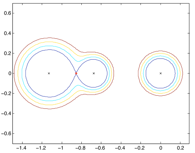
Figure 1: Pseudospectra for the pencil in (25), with eigenvalues marked by the black crosses. Two components of the $\epsilon$-pseudospectrum coalesce for $\epsilon=0.59299$, corresponding to the distance to a nearest pencil with a multiple eigenvalue $\lambda_{\ast}=-0.85488$ at the coalescence point (marked by the asterisk).

8.2 Nearest Rectangular Pencils with at least Two Eigenvalues

As an example for a rectangular pencil, let us consider the $4\times 3$ pencil

$$A-\lambda B=\left[\begin{array}[]{rrr}1&0&0\\ 0&0.1&0\\ 0&2&0.3\\ 0&1&2\\ \end{array}\right]-\lambda\left[\begin{array}[]{ccc}0&0&0\\ 1&0&0\\ 0&1&0\\ 0&0&1\\ \end{array}\right].$$

The KCF of this pencil contains a $4\times 3$ singular block and therefore the pencil has no eigenvalues. However, if the entry ${a}_{22}$ is set to zero, the KCF of the resulting pencil contains a $2\times 1$ singular block and a $2\times 2$ regular block corresponding to finite eigenvalues. Hence, a perturbation with 2-norm $0.1$ is sufficient to have two eigenvalues.

According to the corollaries in Section 5 the distance to the nearest $4\times 3$ pencil with at least two eigenvalues has the characterization

$$\tau_{2}({\mathbb{C}})=\inf_{\mu\in{\mathbb{C}}^{2}}\underbrace{\sup_{\gamma}\sigma_{2m-1}\left(\left[\begin{array}[]{cc}{A}-\mu_{1}{B}&0\\ \gamma{B}&{A}-\mu_{2}{B}\\ \end{array}\right]\right)}_{=:g(\mu)}$$ (26)

for $m=3$. Our implementation returns $\tau_{2}({\mathbb{C}})=0.03927$. The corresponding nearest pencil (16) is given by

$$\left[\begin{array}[]{rrr}0.99847&-0.03697&-0.01283\\ 0&0.08698&0.03689\\ 0&2.00172&0.30078\\ 0.00007&1.00095&2.00376\\ \end{array}\right]-\lambda\left[\begin{array}[]{ccc}0&0&0\\ 1&0&0\\ 0&1&0\\ 0&0&1\\ \end{array}\right]$$

and has eigenvalues at $\mu_{1}=2.55144$ and $\mu_{2}=1.45405$. This result is confirmed by Figure 2, which illustrates the level sets of the function $g(\mu)$ defined in (26) over ${\mathbb{R}}^{2}$.

For this example the optimal $\gamma$ is 2.0086. The smallest three singular values of the matrix in (26) are $1.4832$, $0.0393$ and $0.0062$ for these optimal values of $\mu$ and $\gamma$. The linear independence qualification also holds.

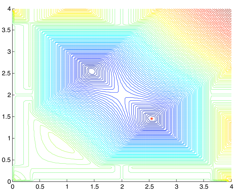
Figure 2: Level sets over $\mathbb{R}^{2}$ of the function $g(\mu)$ defined in (26). The asterisk marks the numerically computed global minimizer of $g$, which corresponds to the eigenvalues of a nearest pencil with two eigenvalues.

8.3 Nearest Stable Pencils

As a last example, suppose that $Bx^{\prime}(t)=Ax(t)$ with $A,B\in{\mathbb{C}}^{n\times n}$ is an unstable descriptor system. The distance to a nearest stable descriptor system is a special case of $\tau_{n}(\Omega)$, with $\Omega={\mathbb{C}}^{-}$, the open left-half of the complex plane. A singular value characterization is given by

$$\tau_{n}({\mathbb{C}}^{-})=\inf_{\lambda_{j}\in{\mathbb{C}}^{-}}\;\;\sup_{\gamma_{ik}\in{\mathbb{C}}}\;\sigma_{n^{2}-n+1}\left(\left[\begin{array}[]{cccc}A-\lambda_{1}B&0&&0\\ \gamma_{21}B&A-\lambda_{2}B&&0\\ &&\ddots&\\ \gamma_{n1}B&\gamma_{n2}B&&A-\lambda_{n}B\\ \end{array}\right]\right).$$

Specifically, we consider a system with $B=I_{2}$ and

$$A=\left[\begin{array}[]{cc}0.6-\frac{1}{3}i&-0.2+\frac{4}{3}i\\ -0.1+\frac{2}{3}i&0.5+\frac{1}{3}i\\ \end{array}\right].$$ (27)

Both eigenvalues $\lambda_{1}=0.7-i$ and $\lambda_{2}=0.4+i$ are in the right-half plane. Based on the singular value characterization, we have computed the distance to a nearest stable system $x^{\prime}(t)=(A+\Delta A_{\ast})x(t)$ as $0.6610$. The corresponding perturbed matrix

$$A+\Delta A_{\ast}=\left[\begin{array}[]{rr}0.0681-0.3064i&-0.4629+1.2524i\\ 0.2047+0.5858i&-0.1573+0.3064i\\ \end{array}\right]$$

at a distance of $0.6610$ has one eigenvalue $\left(\lambda_{\ast}\right)_{1}=-0.0885+0.9547i$ in the left-half plane and the other $\left(\lambda_{\ast}\right)_{2}=-0.9547i$ on the imaginary axis. The $\epsilon$-pseudospectrum of $A$ is depicted in Figure 3. For $\epsilon=0.6610$, one component of the $\epsilon$-pseudospectrum crosses the imaginary axis, while the other component touches the imaginary axis.

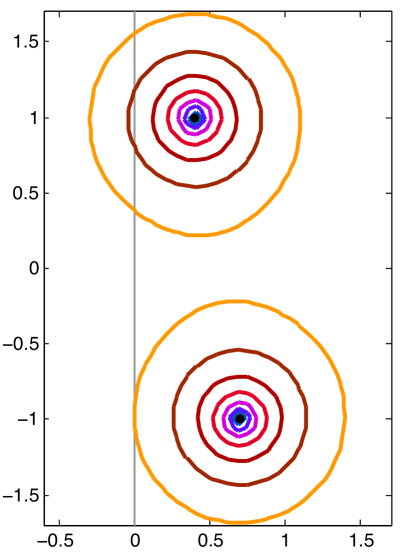
Figure 3: Pseudospectra of the matrix $A$ defined in (27). The outer orange curve represents the boundary of the $\epsilon$-pseudospectrum for $\epsilon=0.6610$, the distance to a nearest stable matrix.

9 Concluding Remarks

In this work a singular value characterization has been derived for the 2-norm of a smallest perturbation to a square or a rectangular pencil $A-\lambda B$ such that the perturbed pencil has a desired set of eigenvalues. The immediate corollaries of this main result are

1. a singular value characterization for the 2-norm of the smallest perturbation so that the perturbed pencil has a specified number of its eigenvalues in a desired region in the complex plane, and

2. a singular value characterization for the 2-norm of the smallest perturbation to a rectangular pencil so that it has a specified number of eigenvalues.

Partly motivated by an application explained in the introduction, we allow perturbations to $A$ only. The extension of our results to the case of simultaneously perturbed $A$ and $B$ remains open.

The development of efficient and reliable computational techniques for the solution of the derived singular value optimization problems is still in progress. As of now the optimization problems can be solved numerically only for small pencils with small number of desired eigenvalues. The main task that needs to be addressed from a computational point of view is a reliable and efficient implementation of the DIRECT algorithm for Lipschitz-based optimization. For large pencils it is necessary to develop Lipschitz-based algorithms converging asymptotically faster than the algorithms (such as the DIRECT algorithm) stemming from the Piyavskii-Shubert algorithm. The derivatives from Section 4.1 might constitute a first step in this direction.

Acknowledgments We are grateful to two anonymous referees for their valuable comments. The research of the second author is supported in part by the European Commision grant PIRG-GA-268355 and the TÜBİTAK (the scientific and technological research council of Turkey) carrier grant 109T660.

Appendix A Proof that $\sigma_{mr-r+1}\left({\mathcal{L}}(\mu,\Gamma,A,B)\right)\to 0$ as $\Gamma\to\infty$

We prove that the $r$ smallest singular values of ${\mathcal{L}}(\mu,\Gamma,A,B)$ decay to zero as soon as at least one entry of $\Gamma$ tends to infinity, provided that $n=m$. In the rectangular case, $n>m$, these singular values generally do not decay to zero.

We start by additionally assuming that $A-\mu_{i}B$ are non–singular matrices for all $i=1,\ldots,r$. We will first prove the result under this assumption, and then we will drop it. Our approach is a generalization of the procedure from [16, §5], which in turn is a generalization of [24, Lemma 2].

Under our assumptions the matrix ${\mathcal{L}}(\mu,\Gamma,A,B)$ is non–singular, and one can explicitly calculate the inverse. It is easy to see that the matrix ${\mathcal{L}}^{-1}(\mu,\Gamma,A,B)$ has the form

$$\begin{bmatrix}(A-\mu_{1}B)^{-1}&0&\ldots&0\\ X_{21}&(A-\mu_{2}B)^{-1}&\ldots&0\\ X_{31}&X_{32}&\ldots&0\\ \vdots&\vdots&\ddots&\vdots\\ X_{r1}&X_{r2}&\ldots&(A-\mu_{r}B)^{-1}\end{bmatrix}.$$

We will use the well–known relations

$$\sigma_{nr-r+1}\left({\mathcal{L}}(\mu,\Gamma,A,B)\right)=\sigma_{r}\left({\mathcal{L}}(\mu,\Gamma,A,B)^{-1}\right)^{-1}\leq\sigma_{r}\left(X_{ij}\right)^{-1}.$$ (28)

We first compute the matrices $X_{21},\ldots,X_{r,r-1}$ which lie on the first sub–diagonal. By a straightforward computation we obtain

$$X_{i+1,i}=-\gamma_{i+1,i}(A-\mu_{i+1}B)^{-1}B(A-\mu_{i}B)^{-1}.$$

If $\sigma_{r}\left((A-\mu_{i+1}B)^{-1}B(A-\mu_{i}B)^{-1}\right)>0$, then from (28) it follows that if any of $|\gamma_{i+1,i}|$ tends to infinity, we obtain the desired result. But $\sigma_{r}\left((A-\mu_{i+1}B)^{-1}B(A-\mu_{i}B)^{-1}\right)>0$ easily follows from the assumption ${\rm rank}(B)\geq r$.

If this is not the case, meaning $\max_{i}\{\gamma_{i+1,i}\}$ is bounded, then we use the entries on the next sub–diagonal $X_{i+2,i}$. Again by straightforward computation we obtain

$$X_{i+2,i}=-\gamma_{i+2,i}(A-\mu_{i+2}B)^{-1}B(A-\mu_{i}B)^{-1}+\gamma_{i+2,i+1}\gamma_{i+1,i}(A-\mu_{i+2}B)^{-1}B(A-\mu_{i+1}B)^{-1}B(A-\mu_{i}B)^{-1}.$$

Because again ${\rm rank}(B)\geq r$ implies $\sigma_{r}\left((A-\mu_{i+2}B)^{-1}B(A-\mu_{i}B)^{-1}\right)>0$, it follows that if any of $|\gamma_{i+2,i}|$ tend to infinity, we obtain the desired result. In general, we have the recursive formula

$$X_{i+j,i}=-\gamma_{i+j,i}(A-\mu_{i+j}B)^{-1}B(A-\mu_{i}B)^{-1}-\sum_{k=1}^{j-1}\gamma_{i+j,i+k}(A-\mu_{i+j}B)^{-1}BX_{i+k,i}.$$

Applying the same procedure as above, we conclude the proof in this case.

To remove the assumption that the matrices $A-\mu_{i}B$ are non–singular, we fix any $\varepsilon>0$. Let us choose a matrix $A_{\varepsilon}$ such that $\|A_{\varepsilon}-A\|<\varepsilon$ and that the matrices $A_{\varepsilon}-\mu_{i}B$ are non–singular for all $i=1,\ldots,r$. From the arguments above, if follows that there exists $\gamma_{0}>0$ such that $\sigma_{nr-r+1}\left({\mathcal{L}}(\mu,\Gamma,A_{\varepsilon},B)\right)<\varepsilon$, when $\|\Gamma\|>\gamma_{0}$. Since

$\sigma_{nr-r+1}\left({\mathcal{L}}(\mu,\Gamma,A,B)\right)\leq\sigma_{nr-r+1}\left({\mathcal{L}}(\mu,\Gamma,A_{\varepsilon},B)\right)+\varepsilon$,

we obtain the inequality $\sigma_{nr-r+1}\left({\mathcal{L}}(\mu,\Gamma,A,B)\right)<2\varepsilon$, when $\|\Gamma\|>\gamma_{0}$.

References

- [1] R. Alam and S. Bora. On sensitivity of eigenvalues and eigendecompositions of matrices. Linear Algebra Appl., 396:273–301, 2005.
- [2] G. Boutry, M. Elad, G. H. Golub, and P. Milanfar. The generalized eigenvalue problem for nonsquare pencils using a minimal perturbation approach. SIAM J. Matrix Anal. Appl., 27(2):582–601, 2005.
- [3] S. Boyd and V. Balakrishnan. A regularity result for the singular values of a transfer matrix and a quadratically convergent algorithm for computing its -norm. Systems Control Lett., 15(1):1–7, 1990.
- [4] A Bunse-Gerstner, R Byers, V. Mehrmann, and N.K. Nichols. Numerical computation of an analytic singular value decomposition of a matrix valued function. Numer. Math., 60:1–39, 1991.
- [5] J. V. Burke, A. S. Lewis, and M. L. Overton. Pseudospectral components and the distance to uncontrollability. SIAM J. Matrix Anal. Appl., 26(2):350–361, 2005.
- [6] R. Byers. A bisection method for measuring the distance of a stable to unstable matrices. SIAM J. Sci. Statist. Comput., 9:875–881, 1988.
- [7] Ralph Byers and N. K. Nichols. On the stability radius of generalized state-space systems. Linear Algebra Appl, 188:113–134, 1993.
- [8] F. De Terán and D. Kressner. Kronecker’s canonical form and the algorithm – revisited. 2012. In preparation.
- [9] J. W. Demmel and A. Edelman. The dimension of matrices (matrix pencils) with given Jordan (Kronecker) canonical forms. Linear Algebra Appl., 230:61–87, 1995.
- [10] R. Eising. Between controllable and uncontrollable. Systems Control Lett., 4(5):263–264, 1984.
- [11] M. Elad, P. Milanfar, and G. H. Golub. Shape from moments—an estimation theory perspective. IEEE Trans. Signal Process., 52(7):1814–1829, 2004.
- [12] J. M. Gablonsky. Modifications of the DIRECT algorithm. PhD thesis, North Carolina State University, Raleigh, North Carolina, 2001.
- [13] F. R. Gantmacher. The Theory of Matrices, volume 1. Chelsea, 1959.
- [14] G. H. Golub and C. F. Van Loan. Matrix Computations. Johns Hopkins University Press, Baltimore, MD, third edition, 1996.
- [15] Kh. D. Ikramov and A. M. Nazari. On the distance to the closest matrix with a triple zero eigenvalue. Mat. Zametki, 73(4):545–555, 2003.
- [16] Kh. D. Ikramov and A. M. Nazari. Justification of a Malyshev–type formula in the nonnormal case. Mat. Zametki, 78(2):241–250, 2005.
- [17] Z. Jia and G. W. Stewart. An analysis of the Rayleigh-Ritz method for approximating eigenspaces. Math. Comp., 70(234):637–647, 2001.
- [18] D. R. Jones, C. D. Perttunen, and B. E. Stuckman. Lipschitzian optimization without the Lipschitz constant. J. Optim. Theory Appl., 79(1):157–181, 1993.
- [19] T. Košir. Kronecker bases for linear matrix equations, with application to two-parameter eigenvalue problems. Linear Algebra Appl., 249:259–288, 1996.
- [20] A. S. Lewis and M. L. Overton. Nonsmooth optimization via BFGS. Math. Program., 2012. to appear.
- [21] R. A. Lippert. Fixing two eigenvalues by a minimal perturbation. Linear Algebra Appl., 406:177–200, 2005.
- [22] R. A. Lippert. Fixing multiple eigenvalues by a minimal perturbation. Linear Algebra Appl., 432(7):1785–1817, 2010.
- [23] D. C. Liu and J. Nocedal. On the limited memory BFGS method for large scale optimization. Math. Programming, 45(3, (Ser. B)):503–528, 1989.
- [24] A. N. Malyshev. A formula for the 2-norm distance from a matrix to the set of matrices with multiple eigenvalues. Numer. Math., 83:443–454, 1999.
- [25] E. Mengi. Locating a nearest matrix with an eigenvalue of prespecified algebraic multiplicity. Numer. Math, 118:109–135, 2011.
- [26] E. Mengi. Nearest linear systems with highly deficient reachable subspaces. 2011. Submitted to SIAM J. Matrix Anal. Appl.
- [27] N. Papathanasiou and P. Psarrakos. The distance from a matrix polynomial to matrix polynomials with a prescribed multiple eigenvalue. Linear Algebra Appl., 429(7):1453–1477, 2008.
- [28] S. A. Piyavskii. An algorithm for finding the absolute extremum of a function. USSR Comput. Math. and Math. Phys., 12:57–67, 1972.
- [29] F. Rellich. Störungstheorie der Spektralzerlegung. I. Analytische Störung der isolierten Punkteigenwerte eines beschränkten Operators. Math. Ann., 113:600–619, 1936.
- [30] B. Shubert. A sequential method seeking the global maximum of a function. SIAM J. Numer. Anal., 9:379–388, 1972.
- [31] K.-C. Toh and L. N. Trefethen. Calculation of pseudospectra by the Arnoldi iteration. SIAM J. Sci. Comput., 17(1):1–15, 1996.
- [32] C. F. Van Loan. How near is a matrix to an unstable matrix? Lin. Alg. and its Role in Systems Theory, 47:465–479, 1984.