PDF modeling of near-wall turbulent flows:
A New model, Weak second-order scheme and a numerical study in a Hybrid configuration

Abstract

In this work, we discuss some points relevant for stochastic modelling of one- and two-phase turbulent flows. In the framework of stochastic modelling, also referred to PDF approach, we propose a new Langevin model including all viscosity effects and thus that is consistent with viscous Navier-Stokes equations. In the second part of the work, we show how to develop a second-order unconditionally stable numerical scheme for the stochastic equations proposed. Accuracy and consistency of the numerical scheme is demonstrated analytically. In the last part of the work, we study the fluid flow in a channel flow with the proposed viscous method. A peculiar approach is chosen: the flow is solved with a Eulerian method and after with the Lagrangian model proposed which uses some of the Eulerian quantities. In this way attention is devoted to the issue of consistency in hybrid Eulerian/Lagrangian methods. It is shown that the coupling is important indeed and that to couple the Lagrangian model to an Eulerian one which is not consistent with the same turbulence physics leads to large errors. This part of the work complements a recent article [Chibbaro and Minier International Journal of Multiphase flows submitted (arXiv:0912.2045)].

1 Introduction

Stochastic modeling approaches (also referred to as Probability Density Function (PDF) methods), once developed in statistical mechanics and solid state physics [1], have been shown to be very powerful for the study of turbulent fluids in presence of complex physics, in particular, for turbulent combustion flows [2] and for polydispersed two-phase flows [3]. The main advantage of the PDF approach over conventional moment-closure methods is its ability to reproduce convection and non-linear source terms without approximations. Moreover, the information available by using such methods is the complete PDF (though modeled) and, thus, all the statistical moments which are related.

In PDF methods, turbulent closure is achieved through a modeled transport equation for the joint PDF of some chosen variables, which constitute the state vector of the process. In this work (and almost ever) the one-particle Lagrangian PDF is considered, from which the one-point one-time joint Eulerian PDF can be extracted. The resulting modeled one-particle PDF transport equation is a Fokker-Planck equation [1], which is a high dimensional scalar equation. Thus, traditional numerical techniques such as finite-volume and finite-difference methods are possible, in theory, but are not suitable to solve PDF equations in practice, since the computational cost increases exponentionally with the number of dimensions. On the other hand, Fokker-Planck equations are equivalent (in a weak sense) to a set of stochastic differential equations (SDEs). In this case, the PDF is represented by an ensemble of Lagrangian stochastic particles whose properties are driven by the model SDEs. These stochastic particles can be regarded as samples of the PDF and following these particles in time represents a dynamical Monte Carlo method, whose computational cost increases only linearly with the number of particles. For this reason, the Monte Carlo method (or particle stochastic approach) is usually chosen to solve high dimensional equations and, in particular, PDF equations.

In turbulent two-phase flows, the SDEs equations of the model contain several mean fields and they have the general form

$$dZ_{i}(t)=A_{i}(t,{\bf Z},\langle f({\bf Z})\rangle)\,dt+\sum_{j}B_{ij}(t,{\bf Z},\langle f({\bf Z})\rangle)\,dW_{j}(t),$$ (1)

where the $\langle\;\rangle$ operator stands for the mathematical expectation. One way to compute mean fields is to extract them directly from the particle properties with the help of a mesh, this is the stand-alone method. This method is fully consistent but suffers, nevertheless, from some drawbacks mainly due to the statistical fluctuations in the particle mean fields[4]. On the other hand, hybrid methods, where the mean fields are provided by a coupled different numerical method, are also possible. These hybrid methods are based on particle-mesh techniques [5]: the mean-field equations are solved on a mesh by standard discretization techniques whereas the dynamics of the particles are still obtained by the time integration of the stochastic differential equations. The main aim of such hybrid methods is to improve the efficiency of numerical simulations without any important loss of accuracy. Indeed, those methods try to conjugate the advantages of moment approach, which provides mean-fields free of statistical errors and low computational costs, with those of PDF one, which are the accurate treatment of some non-linear phenomena and the more detailed level of information.

Recently, the possibility to couple numerical methods of different kind has emerged in several scientific domains, for example the kinetic approach with the fluid one in DSMC simulations [6]. In fluid mechanics, different strategies have been explored to couple PDF methods with other approaches, in particular, Moments/PDF [7, 8], PDF/SPH (smooth particle hydrodynamics)[9] and LES/PDF [10]. In this work, we are dealing with two-phase flows and we choose the framework of hybrid Moments/PDF approach, where, on the one hand, the fluid flow is approached by classical Eulerian moment method and, on the other hand, the dynamics of the solid particles is directly simulated by a stochastic process of the form (1). As mentioned above, the mean fields present in the stochastic model are provided by the Eulerian solver. The present work complements a recent article [11] and thus considers the same configuration treated there that is we limit ourselves to a fluid-fluid configuration, that is, we are considering tracer particles with zero diameter and, as a consequence, zero inertia. This represents an asymptotic limit case of the general two-phase flow configuration, but numerically it preserves the same characteristics concerning the exchange of variables between the different methods and, thus, it gives a privileged position to address issues about the consistency of the method, which is a major point for such approaches and which can be investigated with difficulty in more complex situations. Indeed, in the Eulerian solver, classical second-order turbulent models are generally used, while for the solution of SDEs different techniques must be used, as explained later. In this framework, several mean fields can be computed as duplicate fields in the FV and particle algorithm, which raises questions of consistency. From a numerical point of view, we have chosen a turbulent channel flow as test-case which represents a classical engineering situation.

Three main purposes characterize the present work. The first one is to propose a new viscous PDF model which takes into account the viscous terms that are present in Navier-Stokes equations. This kind of model may be useful when simulations of low-Reynolds number or wall-bounded flows are taken under consideration, since in those cases viscous terms are normally not negligible. The viscous model proposed is shown to be consistent with exact first and second-order moment equations for velocity. The second purpose is to propose a general and rigorous framework in which to develop numerical schemes for SDEs of the very general form (1). In particular, we develop an efficient, stable and accurate numerical schemes for the integration of the trajectories of the stochastic process. This implies two main difficulties.

1. The first one arises from the nature of the stochastic models. SDEs do not obey the rules of classical differential calculus and one has to rely on the theory of stochastic processes [12]. In the present paper, Itô’s calculus is adopted and therefore all SDEs are written in the Itô sense. For stochastic processes, several convergence modes are possible only weak convergence is under consideration, since the purpose is just to estimate mean quantities. A discrete approximation ${\bf Y}_{T}$ ($T$ stands for a given stopping time) converges in the weak sense with order $p$, if for any polynomial $g$, there exists a constant $C$, function of $T$, such that

   $$|\langle g({\bf Z}_{T})\rangle-\langle g({\bf Y}_{T})\rangle|\leqslant C(T)\,\Delta t^{\,p}.$$ (2)

   Due to the mathematical definition of Itô’s integral, numerical schemes developed for PDEs cannot be applied directly.

2. The second difficulty is related to physical constraints. As suggested in Minier [13], the general stochastic model used to simulate general turbulent flows contains several characteristic time-scales. When some of these time-scales become negligible (the system of SDEs is then stiff), various sub-systems of stochastic differential equations can be extracted. In other words, simplified stochastic models can be obtained from the general one. Our second objective is to put forward numerical schemes that can be still applicable, and that remain accurate, when the different time-scales go to zero [14, 8]. Thus, it should be evident that this corresponds to a practical concern, for in the numerical simulation of a complex flow, the time-scales may be negligible in some areas of the flows. We want nevertheless the general numerical scheme to reproduce the correct physical behavior in these areas with the same numerical efficiency. To overlook this point can cause severe problems and even flawed results. For instance, in many studies, wall-bounded flows are considered where SDEs become stiff near the wall. In these cases to use standard numerical schemes like standard euler is not stable. The consequence is that very small time-steps have to be used to stabilise the numerical scheme. That increases much the computational cost, on one hand, and makes results questionable, on the other hand.

The third purpose of this work is to investigate numerically the behavior of the method, even in the asymptotic limits, with the main attention devoted to the issue of consistency. Indeed, hybrid methods are very attractive for simulations of reactive and multiphase flows, but the influence of the exchange of variables remains to be completely understood. It is emphasized here that it is possible to assess the global consistency of the method, because we use a completely consistent and an accurate numerical scheme, which allows us to consider the numerical errors as negligible. Moreover, we will deal with the effect of using not-consistent Eulerian models. Fianlly, a comparison between viscous and high-Reynolds results is carried out.

2 Viscous Model

In this section, we propose a new Langevin model which account for the viscous terms present in the exact PDF equation. Indeed, starting from the exact equations for a fluid, Navier-Stokes equations

$$\frac{\partial U_{j}}{\partial x_{j}}=0,$$ (3a)

$$\frac{\partial U_{i}}{\partial t}+U_{j}\frac{\partial U_{i}}{\partial x_{j}}=-\frac{1}{\rho_{f}}\frac{\partial P}{\partial x_{i}}+\nu\frac{\partial^{2}U_{i}}{\partial x_{j}^{2}},$$ (3b)

we can derive an exact (yet not closed) equation for the one-particle PDF equation for the state-vector ${\bf{Y}}$

$$\begin{split}\frac{\partial f}{\partial t}+V_{i}\frac{\partial f}{\partial x_{i}}=&-\frac{\partial}{\partial V_{i}}[\,\langle-\frac{1}{\rho}\frac{\partial P}{\partial x_{i}}|{\mathbf{Y}}={\mathbf{y}}\rangle\,f\,]\\ &-\frac{\partial}{\partial V_{i}}[\,\langle\nu\Delta U_{i}|{\mathbf{Y}}={\mathbf{y}}\rangle\,f\,],\end{split}$$ (4)

this equation may be considered as the starting point for stochastic modeling. In high-Reynolds number flows, all viscous terms, but the turbulent dissipation, are generally neglected; however, in low-Reynolds number flows or in wall-bounded flows, they can become necessary. In order to include those cases also in the PDF approach, two different Langevin viscous models have been already proposed and tested [15, 16]. Here we propose a third possible model for the state-vector $({\bf x},{\bf U})$:

$$dx_{i} = U_{i}\,dt$$ (5)

$$dU_{i} = -\frac{1}{\rho}\frac{\partial\langle P\rangle}{\partial x_{i}}\,dt+\nu\frac{\partial^{2}\langle U_{i}\rangle}{\partial x^{2}_{k}}\,dt$$ (6)

$$+A_{il}(U_{l}-\langle U_{l}\rangle)\,dt+G_{il}(U_{l}-\langle U_{l}\rangle)\,dt$$

$$+\sqrt{C_{0}\langle\epsilon\rangle}dW_{i},$$

where the matrix $A_{ij}$ is defined implicetely through the equation:

$$(AR)_{ij}=\frac{\nu}{2}\left(\frac{\partial^{2}R_{ij}}{\partial x^{2}_{k}}\right)\,,\text{with}~{}R_{ij}=\langle u_{i}u_{j}\rangle;$$ (7)

and the matrix ${G_{ij}}$ is the general matrix that models the pressure-fluctuation term. In this work, we use the simplified Langevin model (SLM), that is

$$G_{ij}=-\left(\frac{1}{2}+\frac{3}{4}C_{0}\right)\frac{\langle\epsilon\rangle}{k}\;=\;-\frac{1}{T_{L}}~{}.$$ (8)

At last, ${\bf{W}}$ is a Wiener process [1].

This model has been developed in the same framework of the two others cited above, thus, for the general discussion of physical properties of this class of models we refer to those papers. In the appendix A, we show that the model proposed (5)-(6) gives the correct equations for the moments of order 1 (mean-velocity), and 2 (Reynolds-stress) and, therefore, that the model is consistent with the known physics of fluid turbulence.

The main specificity of this new model is that the equation (5) for the position of the stochastic particles is maintained equal to the exact equation of fluid particle-position (in a Lagrangian sense). On the contrary, both other models used the artifice of adding a white noise in the modeled equation of particle position to represent the effect of diffusion. Whilst this feature is only of formal relevance in fluid turbulence, it can be useful in the case of two-phase flows [17], where only this new model can be straightforwardly used. Since the equation for particle position is constrained to remain not-modified, an ad-hoc term has been added in the modeled equation for particle velocity, such that the diffusion in space for mean-velocity and the term constituted by the matrix $A_{ij}$ is necessary to assure the correct equations for the Reynolds-stress. In general flows, the matrix $A_{ij}$ can be computed from the formula (7), that can be rewritten in the form

$${\bf A}\cdot{\bf R}={\bf\epsilon}~{};\text{hence}~{}{\bf A}={\bf\epsilon}\cdot{\bf R}^{-1}~{}.$$ (9)

In present work, we consider the simple case of a channel flow, and further simplifications can be made considering the symmetry properties of Reynolds-stress in x and z directions. Furthermore, we make the hypothesis that the Reynolds-stress are nearly constant in the logarithmic zone, which is well verified experimentally. This is, in fact, an equilibrium hypothesis and, on his basis, we can take just the leading terms in the viscous zone and solve the equation analytically. Then, we have

$$\epsilon=\begin{pmatrix}\frac{\nu}{2}\frac{\partial^{2}\langle u^{2}\rangle}{\partial x^{2}_{i}}&0&0\\ 0&0&0\\ 0&0&\frac{\nu}{2}\frac{\partial^{2}\langle w^{2}\rangle}{\partial x^{2}_{i}}\end{pmatrix}$$ (10)

the resulting matrix $A_{ij}$ has the form

$${\bf A}=\begin{pmatrix}A_{11}&A_{12}&0\\ 0&0&0\\ 0&0&A_{33}\end{pmatrix}$$ (11)

with

$$A_{11} = \frac{\nu}{2}\frac{\partial^{2}\langle u^{2}\rangle}{\partial x^{2}_{i}}\frac{\langle v^{2}\rangle}{\langle u^{2}\rangle\langle v^{2}\rangle-\langle uv\rangle^{2}}$$ (12)

$$A_{12} = -\frac{\nu}{2}\frac{\partial^{2}\langle u^{2}\rangle}{\partial x^{2}_{i}}\frac{\langle uv\rangle}{\langle u^{2}\rangle\langle v^{2}\rangle-\langle uv\rangle^{2}}$$ (13)

$$A_{33} = \frac{\nu}{2}\frac{\partial^{2}\langle w^{2}\rangle}{\partial x^{2}_{i}}\frac{1}{\langle w^{2}\rangle}~{}.$$ (14)

3 Numerical Scheme

Given the physical model, two main issues remain:

1. Numerical integration scheme

2. Boundary conditions for particles

3.1 Stochastic differential system

The set of SDEs to be integrated can be written in a compact form

$$\left\{\begin{split}dx_{i}&=U_{i}\,dt,\\ dU_{i}&=-\frac{1}{T_{i}}U_{i}\,dt+A_{12}U_{2}\delta_{1,i}dt+C_{i}\,dt+\sum_{j}\sigma_{ij}\,dW_{j}(t),\end{split}\right.$$ (15)

where the diffusion matrix is diagonal and is defined

$$\sigma_{ij}(t,{\bf x},\langle{\bf U}\rangle)=\langle\epsilon\rangle C_{0}\delta_{ij},$$ (16)

and vector ${\bf C}$ is the sum of several terms

$$C_{1} = \frac{\langle U_{1}\rangle}{T_{1}}-A_{12}\langle U_{2}\rangle-\frac{1}{\rho}\frac{\partial\langle P\rangle}{\partial x}+\nu\nabla^{2}\langle U_{1}\rangle$$ (17)

$$C_{2} = \frac{\langle U_{2}\rangle}{T_{L}}-\frac{1}{\rho}\frac{\partial\langle P\rangle}{\partial y}+\nu\nabla^{2}\langle U_{2}\rangle$$ (18)

$$C_{3} = \frac{\langle U_{3}\rangle}{T_{3}}-\frac{1}{\rho}\frac{\partial\langle P\rangle}{\partial z}+\nu\nabla^{2}\langle U_{3}\rangle~{},$$ (19)

and the time-scales have become

$$\frac{1}{T_{i}}=\frac{1}{T_{L}}-A_{ii}~{}.$$ (20)

We recall that this model has a physical meaning only in the case where $\eta\ll dt\ll T_{i}$, with $\eta$ the Kolmogorov time-scale. When this condition is not satisfied, it is possible to show that, in the continuous sense (time and all coefficients are continuous functions which can go to zero), the system converges towards several limit systems [13]: case 1: when $T_{i}\rightarrow 0$ with no condition on $\sigma_{ij}T_{i}$, the velocity is no longer random and the system becomes deterministic. The flow is laminar and it can be proven that

$$\text{system (\ref{eq:sysEDS}})\;\xrightarrow[T_{i}\to 0]{}\left\{\begin{split}&dx_{i}=U_{i}\,dt\\ &U_{i}=\langle U_{i}\rangle.\end{split}\right.$$ (21)

That is the expected behavior in the viscous sub-layer.

case 2: When $T_{i}\rightarrow 0$ and at the same time $\sigma_{ij}T_{i}\to cst$ and $A_{1,2}=cst$, the fluid velocity becomes a fast variable. It can be shown that

$$\text{system (\ref{eq:sysEDS})}\;\xrightarrow[T_{i}\to 0]{(\sigma_{ij}T_{i}\to cst)}dx_{i}=\langle U_{i}\rangle\,dt+\sum_{j}(\sigma_{ij}T_{i})\,dW_{j}(t).$$ (22)

We retrieve a pure diffusive behavior, that is the equations of the Brownian motion. Actually, this limit is formal in the continuous sense, being impossible to fit both conditions in a turbulent bounded flow ($\sigma\sim\sqrt{\epsilon}$ which is always bounded). Nevertheless, in numerical computations this limit can be recovered [14] and, furthermore, it has a theoretical relevance, since those conditions are required for the elimination of a variable, treated as fast variable. The same reasoning has been applied to the fluid acceleration to obtain the present model on velocity [3]. Thus, it is important that the numerical scheme is consistent even with this formal limit.

In our model, the diffusion matrix is diagonal, Eq. (16). Although following manipulations are strictly valid for the general case, for the sake of simplicity, from now the diagonal expression will be retained.

3.2 Analytical solutions

The construction of the numerical schemes is now slightly anticipated. Since the numerical methods are derived by freezing the coefficients on the integration intervals, the solutions to system (15), with constant coefficients, are now given.

The method of the constant variation is used. For the fluid velocity with $i\neq 1$, if one seeks a solution of the form $U_{i}(t)=H(t)\exp(-t/T_{i})$, where $H(t)$ is a stochastic process, Itô’s calculus gives

$$dH(t)=\exp(t/T_{i})[C_{i}({\mathbf{x}})\,dt+\sigma_{i}({\mathbf{x}})\,dW_{j}(t)],$$ (23)

that is, by integration on a time interval $[t_{0},t]$ ($\Delta t=t-t_{0}$),

$$\begin{split}U_{i}(t)=U_{i}(t_{0})\exp(-\Delta t/T_{i})+C_{i}&({\mathbf{x}})\,T_{i}\,[1-\exp(-\Delta t/T_{i})]\\ +&\sigma_{i}({\mathbf{x}})\exp(-t/T_{i})\int_{t_{0}}^{t}\exp(s/T_{i})\,dW_{i}(s).\end{split}$$ (24)

We can define

$$\gamma_{i}(t)=\sigma_{i}({\mathbf{x}})\exp(-t/T_{i})\int_{t_{0}}^{t}\exp(s/T_{i})\,dW_{i}(s)~{};\text{for}~{}i\neq 1$$ (25)

For $i=1$ we substitute this expression to $U_{2}$ and we proceed in the same way to obtain

$$\begin{split}&U_{1}(t)=~{}U_{1}(t_{0})\exp(-\Delta t/T_{1})+C_{1}({\mathbf{x}})\,T_{1}\,[1-\exp(-\Delta t/T_{1})]\\ &+A_{12}\exp(-t/T_{1})\int_{t_{0}}^{t}\exp(s/T_{1})\left[U_{2}(t_{0})\exp(-\Delta s/T_{2})+C_{2}({\mathbf{x}})\,T_{2}\,(1-\exp(-\Delta s/T_{2}))+\gamma_{2}(s)\right]ds\\ &+\sigma_{1}({\mathbf{x}})\exp(-t/T_{1})\int_{t_{0}}^{t}\exp(s/T_{1})\,dW_{1}(s).\end{split}$$ (26)

Performing integration by parts we, finally, obtain

$$U_{1}(t) = U_{1}(t_{0})\exp(-\Delta t/T_{1}+[C_{1}({\mathbf{x}})\,T_{1}+C_{2}({\mathbf{x}})\,T_{2}A_{12}T_{2}]\left(1-\exp(-\Delta t/T_{1})\right)$$ (27)

$$+ A_{12}\theta[U_{2}(t_{0})-C_{2}({\mathbf{x}})\,T_{2}]\left[\exp(-\Delta t/T_{2})-\exp(-\Delta t/T_{1})\right]+\gamma_{1}(t)$$

having defined

$$\gamma_{1}(t) = A_{12}\exp(-t/T_{1})\int_{t_{0}}^{t}\exp(s/T_{1})\gamma_{2}(s)ds+\sigma_{1}\exp(-t/T_{1})\int_{t_{0}}^{t}\exp(s/T_{1})dW_{1}$$ (28)

$$\theta = \frac{T_{1}T_{2}}{T_{2}-T_{1}}~{}.$$ (29)

The first integral in the definition of $\gamma_{1}$ is a double stochastic integral which can be simplified through the integration by parts, as explained in appendix B.1. The new formula is

$$\gamma_{1}(t) = A_{12}\sigma_{2}\theta\left[\exp(-t/T_{2})\int_{t_{0}}^{t}\exp(s/T_{2})dW_{2}-\exp(-t/T_{1})\int_{t_{0}}^{t}\exp(s/T_{1})dW_{2}\right]$$ (30)

$$+ \sigma_{1}\exp(-t/T_{1})\int_{t_{0}}^{t}\exp(s/T_{1})dW_{1}$$

The analytical solutions for the positions are worked out is a similar manner starting from Eq. (5)

$$dx_{i}=U_{i}dt\Rightarrow x_{i}(t)=x_{i}(t_{0})+\int_{t_{0}}^{t}U_{i}(s)ds$$ (31)

for $i\neq 1$

$$x_{i}(t) = x_{i}(t_{0})+U_{i}(t_{0})T_{i}[1-\exp(-\Delta t/T_{i})]+[C_{i}({\mathbf{x}})T_{i}]\{\Delta t-T_{i}[1-\exp(-\Delta t/T_{i})]\}+\Gamma_{1}(t)$$ (32)

$$\Gamma_{i}(t) = \sigma_{i}\int_{t_{0}}^{t}\exp(-t^{\prime}/T_{i})\int_{t_{0}}^{t^{\prime}}\exp(s/T_{i})dW_{i}(s)$$ (33)

As usual, the double integral can be transformed

$$\Gamma_{i}(t)=\sigma_{i}T_{i}\left[\int_{t_{0}}^{t}dW_{i}(s)-\exp(-t/T_{i})\int_{t_{0}}^{t}\exp(s/T_{i})dW_{i}(s)\right]~{};~{}\text{for}~{}i=\{2,3\}~{}.$$ (34)

Finally, the integration of the first component in position gives

$$x_{1}(t) = x_{1}(t_{0})+U_{1}(t_{0})T_{1}[1-\exp(-\Delta t/T_{1})]+T_{1}[C_{1}({\mathbf{x}})+A_{12}C_{2}({\mathbf{x}})T_{2}]\times$$ (35)

$$\times \{\Delta t-T_{1}[1-\exp(-\Delta t/T_{1})]\}+A_{12}\theta[U_{2}(t_{0})-C_{2}({\mathbf{x}})T_{2}]\times$$

$$\times [T_{2}(1-\exp(-\Delta t/T_{2}))-T_{1}(1-\exp(-\Delta t/T_{1}))]+\Gamma_{1}(t)$$

$$\Gamma_{1}(t) = A_{12}\sigma_{2}\theta\left\{(T_{2}-T_{1})\int_{t_{0}}^{t}dW_{2}(s)-T_{2}\exp(-t/T_{2})\int_{t_{0}}^{t}\exp(s/T_{2})dW_{2}(s)\right.$$ (36)

$$+ \left.T_{1}\exp(-t/T_{1})\int_{t_{0}}^{t}\exp(s/T_{1})dW_{2}(s)\right\}$$

$$+ \sigma_{1}\left[\int_{t_{0}}^{t}dW_{1}-T_{1}\exp(-t/T_{1})\int_{t_{0}}^{t}\exp(s/T_{1})dW_{1}(s)\right]~{};$$

also for the position the stochastic integral $\Gamma_{1}$ has been reduced in his basic components through integration by parts. To conclude this section, we resume all the analytical solutions in table 1.

The stochastic integrals, Eqs (52) to (55) in Table 1, only for the constant coefficient case, are Gaussian processes since they are stochastic integrals of deterministic functions [12]. These integrals are quite involved, but, actually, they are expressed in function of some simple stochastic integrals which can be used as base. The base is formed by the following 7 integrals

$$I_{1,i} = \exp(-t/T_{i})\int_{t_{0}}^{t}\exp(s/T_{i})dW_{i}(s)\quad i=\{1,2,3\}$$ (37)

$$I_{2,2} = \exp(-t/T_{1})\int_{t_{0}}^{t}\exp(s/T_{1})dW_{2}(s)$$ (38)

$$I_{3,i} = \int_{t_{0}}^{t}dW_{i}(s)\quad i=\{1,2,3\}~{}.$$ (39)

The original stochastic integrals eqs (52) to (55) are, then, decomposed and reformulated as

$$\text{i$\neq$1}\quad\quad\gamma_{i} = \sigma_{i}I_{1,1}$$ (40)

$$\text{i=1}\quad\quad\gamma_{1} = A_{12}\sigma_{2}\theta[I_{1,2}-I_{2,2}]+\sigma_{1}I_{1,1}$$ (41)

$$\text{i$\neq$1}\quad\quad\Gamma_{i} = \sigma_{i}T_{i}[I_{3,1}-I_{1,i}]$$ (42)

$$\text{i=1}\quad\quad\Gamma_{1} = A_{12}\sigma_{2}\theta[(T_{2}-T_{1})I_{3,2}-T_{2}I_{1,2}+T_{1}I_{2,2}]+\sigma_{1}T_{1}[I_{3,1}-I_{1,1}]~{}.$$ (43)

In a matrix form the two set of integrals are related by the formula

$$\begin{pmatrix}\gamma_{1}\\ \vdots\\ \Gamma_{3}\end{pmatrix}={\bf M}\cdot\begin{pmatrix}I_{1,1}\\ \vdots\\ I_{3,3}\end{pmatrix}$$ (44)

with

$${\bf M}=\begin{bmatrix}\sigma_{1}&A_{12}\sigma_{2}\theta&0&-A_{12}\sigma_{2}\theta&&\dots&0\\ 0&\sigma_{2}&0&\dots&&\dots&0\\ 0&0&\sigma_{3}&&\dots&&0\\ -\sigma_{1}T_{1}&-T_{2}A_{12}\sigma_{2}\theta&0&T_{1}A_{12}\sigma_{2}\theta&\sigma_{1}T_{1}&(T_{2}-T_{1})A_{12}\sigma_{2}\theta&0\\ 0&-\sigma_{2}T_{2}&0&0&0&\sigma_{2}T_{2}&0\\ 0&0&-\sigma_{3}T_{3}&0&0&0&\sigma_{3}T_{3}\end{bmatrix}$$ (45)

In order to evaluate and to simulate numerically stochastic integrals, it is necessary to compute the moments of integrals and in particular the covariance matrix $C_{ij}$. Here, we do not proceed to the complicated calculation of the covariance matrix of the integrals $\Gamma$ and $\gamma$, but we compute the simpler covariance matrix of the base integrals (37)-(39). Once computed this covariance matrix and with the help of the relations given by Eqs. (44)-(45), it always possible to retrieve the covariance of $\Gamma$ and $\gamma$ and, then, to simulate them numerically. The covariance matrix of the base integrals (37)-(39) is obtained using the techniques explained in appendix B.2 and the resulting values are shown in table 2.

Again, we slightly anticipate the numerics and it is explained how the stochastic integrals can be calculated (simulated). It has just been shown that these integrals are Gaussian processes whose means and variances are know (zero mean and covariance matrix given by Table 2). The vector composed by the seven stochastic integrals, eqs (37) to (39), is a vector of Gaussian centered random variables which can be computed by resorting to the simulation of a vector composed of independent normal Gaussian variables (zero mean and variance equal to one). This technique, which requires the Choleski decomposition of the covariance matrix, is displayed in Appendix C. It is worth recalling that once computed the stochastic integrals forming our base, the integrals (52)-(55) can be obtained through the matrix relation (44).

At last, let us check that the expressions of Table 1 and 2 are consistent with the limit cases given, in the continuous sense.

case 1: when $T_{i}\rightarrow 0$ with no condition on $\sigma_{i}$, the flow becomes laminar, which means that the system becomes deterministic, see Eq. (21). Once again, the results given by Table 1 and 2 are in agreement with Eq. (21). When $T_{i}\rightarrow 0$, eqs (48) to (51) become

$$\begin{split}&U_{i}(t)=\langle U_{i}(t)\rangle,\\ &x_{i}(t)=x_{i}(t_{0})+\langle U_{i}(t)\rangle\Delta t,\end{split}$$ (46)

which is the analytical solution to system (22) when the coefficients are constant.

case 2: When $T_{i}\rightarrow 0$ and at the same time $\sigma_{i}T_{i}\to cst$, we have

$$dx_{i}=\langle U_{i}\rangle\,dt+\sigma_{i}T_{i}\sqrt{\Delta t}{\mathcal{G}}_{i}~{}$$ (47)

where ${\mathcal{G}}_{i}$ is ${\mathcal{N}}(0,1)$ vector (a vector composed of independent normal Gaussian random variables).

A major conclusion can be derived, in order to have a consistent and stable numerical scheme for the integration, even within the asymptotic limits, it is necessary to retain the exponential terms in the solution and all the stochastic integrals, even the indirect ones, must be explicitly calculated.

Table 1: Analytical solutions to system (15) for time-independent coefficients.

 

$$x_{1}(t) =x_{1}(t_{0})+U_{1}(t_{0})T_{1}[1-\exp(-\Delta t/T_{1})]+T_{1}[C_{1}({\mathbf{x}})+A_{12}C_{2}({\mathbf{x}})T_{2}]\times$$

$$\times\{\Delta t-T_{1}[1-\exp(-\Delta t/T_{1})]\}+A_{12}\theta[U_{2}(t_{0})-C_{2}({\mathbf{x}})T_{2}]\times$$

$$\times[T_{2}(1-\exp(-\Delta t/T_{2}))-T_{1}(1-\exp(-\Delta t/T_{1}))]+\Gamma_{1}(t)$$ (48)

$$x_{i}(t) =x_{i}(t_{0})+U_{i}(t_{0})T_{i}[1-\exp(-\Delta t/T_{i})]+[C_{i}({\mathbf{x}})T_{i}]\{\Delta t-T_{i}[1-\exp(-\Delta t/T_{i})]\}$$

$$+\Gamma_{1}(t)$$ (49)

$$U_{1}(t) =U_{1}(t_{0})\exp(-\Delta t/T_{1}+[C_{1}({\mathbf{x}})\,T_{1}+C_{2}({\mathbf{x}})\,T_{2}A_{12}T_{2}]\left(1-\exp(-\Delta t/T_{1})\right)$$

$$+A_{12}\theta[U_{2}(t_{0})-C_{2}({\mathbf{x}})\,T_{2}]\left(\exp(-\Delta t/T_{2}-\exp(-\Delta t/T_{1}\right)+\gamma_{1}(t)$$ (50)

$$U_{i}(t) =U_{i}(t_{0})\exp(-\Delta t/T_{i})+C_{i}({\mathbf{x}})\,T_{i}\,[1-\exp(-\Delta t/T_{i})]$$

$$+\sigma_{i}({\mathbf{x}})\exp(-t/T_{i})\int_{t_{0}}^{t}\exp(s/T_{i})\,dW_{i}(s)$$ (51)

The stochastic integrals $$\gamma_{i}(t),\;\Gamma_{i}(t),$$ are given by:

$$\Gamma_{1}(t) =A_{12}\sigma_{2}\theta\left[(T_{2}-T_{1})\int_{t_{0}}^{t}dW_{2}(s)-T_{2}\exp(-t/T_{2})\int_{t_{0}}^{t}\exp(s/T_{2})dW_{2}(s)\right.$$

$$+\left.T_{1}\exp(-t/T_{1})\int_{t_{0}}^{t}\exp(s/T_{1})dW_{2}(s)\right]$$

$$+\sigma_{1}\left[\int_{t_{0}}^{t}dW_{1}-T_{1}\exp(-t/T_{1})\int_{t_{0}}^{t}\exp(s/T_{1})dW_{1}(s)\right]$$ (52)

$$\Gamma_{i}(t) =\sigma_{i}T_{i}\left[\int_{t_{0}}^{t}dW_{i}(s)-\exp(-t/T_{i})\int_{t_{0}}^{t}\exp(s/T_{i})dW_{i}(s)\right]~{};~{}\text{for}~{}i=\{2,3\}$$ (53)

$$\gamma_{1}(t) =A_{12}\exp(-t/T_{1})\int_{t_{0}}^{t}\exp(s/T_{1})\gamma_{2}(s)ds+\sigma_{1}\exp(-t/T_{1})\int_{t_{0}}^{t}\exp(s/T_{1})dW_{1}$$ (54)

$$\gamma_{i}(t) =\sigma_{i}({\mathbf{x}})\exp(-t/T_{i})\int_{t_{0}}^{t}\exp(s/T_{i})\,dW_{i}(s)$$ (55)

 

Table 2: Derivation of the covariance matrix for constant coefficients.

 

$$\langle I_{1,i}^{2}(t)\rangle=\frac{T_{i}}{2}\left[1-\exp(-2\Delta t/T_{i})\right]$$ (56)

$$\langle I_{2,2}^{2}(t)\rangle=\frac{T_{1}}{2}\left[1-\exp(-2\Delta t/T_{1})\right]$$ (57)

$$\langle I_{3,i}^{2}(t)\rangle=\Delta t$$ (58)

$$\langle I_{1,i}I_{3,i}\rangle=T_{i}\left[1-\exp(-\Delta t/T_{i})\right]$$ (59)

$$\langle I_{1,2}I_{2,2}\rangle=\frac{T_{2}T_{1}}{T_{2}+T_{1}}\left[1-\exp(-\Delta t/T_{1})\exp(-\Delta t/T_{2})\right]$$ (60)

$$\langle I_{2,2}I_{3,2}\rangle=T_{1}\left[1-\exp(-\Delta t/T_{1})\right]$$ (61)

 

Table 3: Weak first order scheme (Euler scheme): sch1

 

$$\text{\text@underline{Numerical integration of the system}}:$$

$$\text{i$\neq$1}\quad x_{i}^{n+1}=x_{i}^{n}+A\,U_{i}^{n}+B\,T_{i}^{n}C_{i}^{n}+\Gamma_{i}^{n},$$

$$\text{i=1}\quad x_{1}^{n+1}=x_{1}^{n}+A\,U_{1}^{n}+B\,T_{1}^{n}[C_{1}^{n}+A_{12}^{n}C_{2}^{n}T-2^{n}]+C\,A_{12}^{n}[U_{2}^{n}-C_{2}^{n}T_{2}^{n}]+\Gamma_{1}^{n},$$

$$\text{i$\neq$1}\quad U_{i}^{n+1}=U_{i}^{n}\,\exp(-\Delta t/T_{i}^{n})+[T_{i}^{n}C_{i}^{n}]D[1-\exp(-\Delta t/T_{i}^{n})]+\gamma_{i}^{n},$$

$$\text{i=1}\quad U_{i}^{n+1}=U_{i}^{n}\,\exp(-\Delta t/T_{1}^{n})+T_{1}^{n}[C_{1}^{n}+A_{12}^{n}C_{2}^{n}T_{2}^{n}]D+[U_{2}^{n}-C_{2}^{n}T_{2}^{n}]E+\gamma_{i}^{n},$$

$$\text{\text@underline{The coefficients $A,\;B,\;C,\;D$ and $E$ are given by}}:$$

$$\quad A=T_{i}^{n}(1-\exp(-\Delta t/T_{i}^{n})$$

$$\quad B=\Delta t-A$$

$$\quad C=\theta^{n}[T_{2}^{n}(1-\exp(-\Delta t/T_{2}^{n}))-T_{1}^{n}(1-\exp(-\Delta t/T_{1}^{n}))]\quad\text{with}\quad\theta^{n}=\frac{T_{2}^{n}T_{1}^{n}}{T_{2}^{n}-T_{1}^{n}}$$

$$\quad D=[1-\exp(-\Delta t/T_{i}^{n})]$$

$$\quad E=A_{12}^{n}\theta^{n}\left(\exp(-\Delta t/T_{2}^{n})-\exp(-\Delta t/T_{1}^{n})\right)$$

 

3.3 Constraints of the numerical schemes

In the particle-mesh method adopted here, the PDEs for the fluid are first solved and then the dynamics of the stochastic particles is computed. Thus, the scheme has to be explicit. Furthermore, the time step, which should be the same for the integration of the PDEs and the SDEs, is imposed by stability conditions required by the Eulerian integration operator. This implies that, since there is no possibility to control the time step when integrating the SDEs, the numerical scheme has to be unconditionally stable. At last, since particle localization in a mesh is CPU demanding, the numerical scheme should minimize these operations. The first constraint is

1. The numerical scheme must be explicit, stable, of order $2$ in time and the number of calls to particle localization has to be minimum.

A practical strategy to fulfill the stability condition is to base the scheme on the analytical solutions presented in Section 3.2. Indeed, the time step appears in decaying exponentials of the type $\exp(-\Delta t)$, which brings unconditional stability. Therefore, the second constraint is

1. The numerical scheme must be consistent with the analytical solutions of the system when the coefficients are constant.

1. The numerical scheme must be consistent with all limit systems.

For a general and comprehensive discussion about the delicate point of asymptotic limit, we refer to the paper [8], where this issue is analyzed in the more general case of two-phase flows. The construction of the scheme on the analytical solutions should also ensure a sound physical treatment of the multi-scale character of the problem. Indeed, it has been demonstrated that from the analytical solutions given in Section 3.2, the limit cases can be retrieved.

3.4 Weak first-order scheme

The derivation of the weak first order scheme is rather straightforward since the analytical solutions of system (15) with constant coefficients have been evaluated. Indeed, the Euler scheme (which is a weak scheme of order $1$ [18]) is simply obtained by freezing the coefficients at the beginning of the time intervals $\Delta t=[t_{n},t_{n+1}]$. Let $Z_{i}^{n}$ and $Z_{i}^{n+1}$ be the approximated values of $Z_{i}$ at time $t_{n}$ and $t_{n+1}$. The Euler scheme is then simply written by using the results of Tables 1 and 2 as shown in Table 3. This scheme fulfills all criteria listed in Section 3.3, except, of course, the order of convergence in time.

As far as the consistency with all limit systems is concerned, some precisions must be given. Here, it has to be understood that the limit systems are presented in the discrete sense. The observation time scale $dt$ has now become the time step $\Delta t$. The physical time scale $T_{i}$ does not go to zero, as in the continuous sense, but its value, depending on the history of the particles, can be smaller or greater than $\Delta t$.

In the limit case 1 (21) we have, with $1\ll\Delta t/T_{i}$,

$$\Gamma_{i}(t) \xrightarrow[T_{i}\to 0]{}\sigma_{i}\,T_{i}\sqrt{\Delta t}{\mathcal{G}}_{x,i}\approx 0$$ (63)

$$\gamma_{i}(t) \xrightarrow[T_{i}\to 0]{}0$$ (64)

and, thus, for the fluid variables

$$U_{i}^{n+1} = \langle U_{i}^{n}\rangle$$ (65)

$$x^{n+1}_{i} = x_{i}^{n}+\langle U_{i}^{n}\rangle\Delta t~{}.$$ (66)

In this case these relations are identical to those analytic. In the second limit case (22) it is different; for the present scheme, Eq. (51), with $1\ll\Delta t/T_{i}$ and the constraints on $\sigma$, gives

$$U_{i}^{n+1}=\langle U_{i}^{n}\rangle+\sqrt{\frac{\sigma_{i}^{n2}\,T_{i}^{n}}{2}}\;\;{\mathcal{G}}_{1,i},$$ (67)

From the continuous point of view, the fluid velocity $U_{i}$ will behave as a fast variable and a near white-noise term. On the contrary, in the numerical simulation, the velocity $U_{i}$ does not, of course, behave strictly-speaking as white-noise function (its variance is not infinite!). This result is physically sound. Indeed, when a fluctuating physical process (random variable) is observed at time steps which are greater that its memory, the expected behavior is Gaussian. For particle position the scheme gives

$$x^{n+1}_{i}=x^{n}_{i}+\langle U^{n}_{i}\rangle\Delta t++\sqrt{\sigma_{i}^{n2}\,T_{i}^{n2}\,\Delta t}\;\;{\mathcal{G}}_{x,i},$$ (68)

as expected.

3.5 Weak second order scheme

3.5.1 Property of the system

The diffusion matrix of system (15) has a singular property, that has a crucial importance here [14]. From Eq. (16), it can be noticed that $\sigma_{ij}$ depends only on time, position and the mean value of the relative velocity. Therefore, the only variable of the state vector whose $\sigma_{ij}$ is a function is ${{\mathbf{x}}}_{p}$. Therefore, the diffusion matrix has the following singular property

$$\sum_{k}\sum_{j}\sigma_{kj}\,\frac{\partial\sigma_{ij}}{\partial x_{k}}=0,\quad\forall\;(i).$$ (69)

3.5.2 General method

Let us consider, for a moment, the following stochastic differential equation

$$dX_{i}(t)=A_{i}({\mathbf{X}}(t))\,dt+\sum_{j}B_{ij}({\mathbf{X}}(t))\,dW_{j}(t)$$

where ${{\mathbf{A}}}$ is the drift vector and ${{\mathbf{B}}}$ is the diffusion matrix. If ${{\mathbf{B}}}$ verifies the property (69), it can be shown that, for example by stochastic Taylor expansions [18], a prediction-correction scheme of the type

$$\begin{split}&{\boldsymbol{t}}_{2}{X}_{i}^{n+1}=X_{i}^{n}+A_{i}^{n}\,dt+\sum_{j}B_{ij}^{n}\,\Delta W_{j},\\ &X_{i}^{n+1}=X_{i}^{n}+\frac{1}{2}\left(A_{i}^{n}+{\boldsymbol{t}}_{2}{A}_{i}^{n+1}\right)\,dt+\sum_{j}\frac{1}{2}\left(B_{ij}^{n}+\tilde{B}_{ij}^{n+1}\right)\,\Delta W_{j},\end{split}$$ (70)

is a weak second order scheme (${\boldsymbol{t}}_{2}{A}_{i}^{n+1}=A_{i}({\boldsymbol{t}}_{2}{{\mathbf{X}}}^{n+1})$ and ${\boldsymbol{t}}_{2}{B}_{ij}^{n+1}=B_{ij}({\boldsymbol{t}}_{2}{{\mathbf{X}}}^{n+1})$). This result is true, one again, only when the property (69) is verified. If not, other terms are needed in order to obtain a weak second order scheme, see for example Talay [19]. As a consequence, it this scheme is used for a set of stochastic equations which do not verify the property (69), problems of consistency arise [20].

The idea is now to built from Eq. (70) a weak second order scheme for system (15). The first-order Euler scheme is going to be used as a prediction step. The remaining task consists in finding a suitable correction step which enforces the three conditions listed in Section 3.3.

3.5.3 Implementation of the scheme

The main idea for the implementation of the correction step is to start from the analytical solutions to system (15) when the coefficients are constant and apply the same idea as in Eq. (70) considering that the acceleration terms vary linearly with time.

Before the implementation of the numerical scheme, let us specify the notation which is in use. As in Section 3.4, $Z_{i}^{n}$ and $Z_{i}^{n+1}$ stand for the approximated values of $Z_{i}$ at time $t_{n}$ and $t_{n+1}$, respectively. Therefore, $Z_{i}^{n+1}$ is the corrected value whereas the predicted value is denoted ${\boldsymbol{t}}_{2}{Z}_{i}^{n+1}$, i.e. the value of $Z_{i}$ predicted by the Euler scheme. The predicted velocities are ${\boldsymbol{t}}_{2}{U}_{i}^{n+1}$ and the values of the fields taken at $(t_{n+1},\,{\mathbf{x}}^{n+1})$ are denoted, for example, $\langle P^{n+1}\rangle$. The predicted time scales are referred to as ${\boldsymbol{t}}_{2}{T}_{i}^{n+1}$ and the predicted diffusion matrix is designated by ${\boldsymbol{t}}_{2}{\sigma}_{i}^{n+1}$.

As far as the computation of the fields ’attached’ to the particles are concerned, it is worth emphasizing that none of them are computed at $(t_{n+1},\,{\mathbf{x}}^{n+1})$, because the scheme would become implicit. All fields which characterize the fluid, such as the mean pressure field, are taken at $(t_{n+1},\,{\mathbf{x}}^{n+1})$, but fields such as the expected value of the fluid velocity are computed from the predicted velocities. For example, one has

$$C_{i}(t_{n+1},\,{\mathbf{x}}^{n+1})={{\boldsymbol{t}}_{2}{C}_{i}^{n+1}}=\frac{1}{{\boldsymbol{t}}_{2}{T}_{i}^{n+1}}\langle U_{i}^{n+1}\rangle+\Pi_{i}(\langle{\mathbf{U}}^{n+1}\rangle,\langle P^{n+1}\rangle).$$

The analytical solution to system (15) when the coefficients are constant is, for the fluid velocity seen, by applying the rules of Itô’s calculus

$$\text{i$\neq$1}\quad U_{i}(t)=U_{i}(t_{0})\,\exp(-\Delta t/T_{i})+\int_{t_{0}}^{t}C_{i}(s)\exp[(s-t)/T_{i}]\,ds+\gamma_{i}(t).$$ (71)

As anticipated we suppose that the acceleration $C_{i}(s,{\mathbf{x}}_{p})$ varies linearly on the integration interval $[t_{0},t]$, that is

$$C_{i}(s,{\mathbf{x}}(s))=C_{i}(t_{0},{\mathbf{x}}(t_{0}))+\frac{1}{\Delta t}[C_{i}(t,{\mathbf{x}}(t))-C_{i}(t_{0},{\mathbf{x}}(t_{0}))](s-t_{0}).$$ (72)

By direct integration, one can write

$$U_{i}(t)=U_{i}(t_{0})\,\exp(-\Delta t/T_{i})+[T_{i}\,C_{i}(t_{0},{\mathbf{x}}(t_{0}))]\,A(\Delta t,T_{i})+[T_{i}\,C_{i}(t,{\mathbf{x}}(t))]\,B(\Delta t,T_{i})+\gamma_{i}(t),$$

where the functions $A(\Delta t,X)$ and $B(\Delta t,X)$ are given by

$$\begin{split}&A(\Delta t,X)=-\exp(-\Delta t/X)+\left[\frac{1-\exp(-\Delta t/X)}{\Delta t/X}\right],\\ &B(\Delta t,X)=1-\left[\frac{1-\exp(-\Delta t/X)}{\Delta t/X}\right].\end{split}$$ (73)

By direct application of the ideas presented in the last section, it is proposed to write

$$\begin{split}U_{i}^{n+1}=&\frac{1}{2}\,U_{i}^{n}\,\exp(-\Delta t/T_{i}^{n})+\frac{1}{2}\,U_{i}^{n}\,\exp(-\Delta t/{\boldsymbol{t}}_{2}{T}_{i}^{n+1})\\ +&A(\Delta t,\,T_{i}^{n})\,[T_{i}^{n}C_{i}^{n}]+B(\Delta t,\,{\boldsymbol{t}}_{2}{T}_{i}^{n+1})\,[{\boldsymbol{t}}_{2}{T}_{i}^{n+1}{\boldsymbol{t}}_{2}{C}_{i}^{n+1}]+{\boldsymbol{t}}_{2}{\gamma}_{i}^{n+1},\end{split}$$ (74)

The meaning of the corrected stochastic integrals will be given later. For the first components the exact solution is

$$\begin{split}\text{i$=$1}\quad U_{1}(t)=&U_{1}(t_{0})\,\exp(-\Delta t/T_{1})+\int_{t_{0}}^{t}C_{1}(s)\exp[(s-t)/T_{1}]\,ds\\ +&\int_{t_{0}}^{t}A_{12}U_{2}(s)\exp[(s-t)/T_{1}]ds+\int_{t_{0}}^{t}\exp[(s-t)/T_{1}]\sigma_{1}(s)dW_{1}(s)~{}.\end{split}$$ (75)

Here, we introduce the exact expression for the variable $U_{2}$

$$U_{2}(t)=U_{2}(t_{0})\,\exp(-\Delta t/T_{2})+\int_{t_{0}}^{t}C_{i}(s)\exp[(s-t)/T_{2}]\,ds+\gamma_{2}(t).$$ (76)

and, then, we let the functions $C_{i}$ and $\sigma$ varying linearly. The subsequent integration, quite involved, permit us to propose the following expression

$$\begin{split}U_{1}^{n+1}=&\frac{1}{2}\,U_{1}^{n}\,\exp(-\Delta t/T_{1}^{n})+\frac{1}{2}\,U_{1}^{n}\,\exp(-\Delta t/{\boldsymbol{t}}_{2}{T}_{1}^{n+1})+\frac{1}{2}U_{2}^{n}A_{12}^{n}E(T_{1}^{n},T_{2}^{n})\\ +&A(\Delta t,\,T_{1}^{n})\,[T_{1}^{n}C_{1}^{n}]+B(\Delta t,\,{\boldsymbol{t}}_{2}{T}_{1}^{n+1})\,[{\boldsymbol{t}}_{2}{T}_{1}^{n+1}{\boldsymbol{t}}_{2}{C}_{1}^{n+1}]\\ +&A_{12}^{n}[T_{2}^{n}C_{2}^{n}]A_{c}(T_{1}^{n},T_{2}^{n})+{\boldsymbol{t}}_{2}{A}_{12}^{n}[{\boldsymbol{t}}_{2}{T}_{2}^{n+1}{\boldsymbol{t}}_{2}{C}_{2}^{n+1}]B_{c}(T_{1}^{n},T_{2}^{n})+{\boldsymbol{t}}_{2}{\gamma}_{1}^{n+1}~{}.\end{split}$$ (77)

where the functions $A_{c}(X,Y)$ and $B_{c}(X,Y)$ are given by

$$\begin{split}&A_{c}(X,Y)=-\exp(-\Delta t/X)+\frac{X+Y}{\Delta t}[1-\exp(-\Delta t/X)]-\left(1+\frac{Y}{\Delta t}\right)\,C_{c}(X,Y),\\ &B_{c}(X,Y)=1-\frac{X+Y}{\Delta t}[1-\exp(-\Delta t/X)]+\frac{Y}{\Delta t}\,C_{c}(X,Y).\\ &\text{with}\\ &C_{c}(X,Y)=\frac{Y}{Y-X}\,[\exp(-\Delta t/Y)-\exp(-\Delta t/X)],\\ \end{split}$$

Table 4: Weak second order scheme: sch2c

 

Prediction step:

$$\text{apply the Euler scheme Sch1, see Table \ref{tab:sch1}}.$$

Correction step:

$$U_{1}^{n+1}=\frac{1}{2}\,U_{1}^{n}\,\exp(-\Delta t/T_{1}^{n})+\frac{1}{2}\,U_{1}^{n}\,\exp(-\Delta t/{\boldsymbol{t}}_{2}{T}_{1}^{n+1})+\frac{1}{2}U_{2}^{n}A_{12}^{n}E(T_{1}^{n},T_{2}^{n})$$

$$+A(\Delta t,\,T_{1}^{n})\,[T_{1}^{n}C_{1}^{n}]+B(\Delta t,\,{\boldsymbol{t}}_{2}{T}_{1}^{n+1})\,[{\boldsymbol{t}}_{2}{T}_{1}^{n+1}{\boldsymbol{t}}_{2}{C}_{1}^{n+1}]$$

$$+A_{12}^{n}[T_{2}^{n}C_{2}^{n}]A_{c}(T_{1}^{n},T_{2}^{n})+{\boldsymbol{t}}_{2}{A}_{12}^{n}[{\boldsymbol{t}}_{2}{T}_{2}^{n+1}{\boldsymbol{t}}_{2}{C}_{2}^{n+1}]B_{c}(T_{1}^{n},T_{2}^{n})+{\boldsymbol{t}}_{2}{\gamma}_{1}^{n+1}~{}.$$

$$U_{i}^{n+1}=\frac{1}{2}\,U_{i}^{n}\,\exp(-\Delta t/T_{i}^{n})+\frac{1}{2}\,U_{i}^{n}\,\exp(-\Delta t/{\boldsymbol{t}}_{2}{T}_{i}^{n+1})$$

$$+A(\Delta t,\,T_{i}^{n})\,[T_{i}^{n}C_{i}^{n}]+B(\Delta t,\,{\boldsymbol{t}}_{2}{T}_{i}^{n+1})\,[{\boldsymbol{t}}_{2}{T}_{i}^{n+1}{\boldsymbol{t}}_{2}{C}_{i}^{n+1}]+{\boldsymbol{t}}_{2}{\gamma}_{i}^{n+1}$$

$$\text{\text@underline{The coefficients $A,\;B,\;A_{c},\;B_{c}$ et $C_{c}$ are defined as}}:$$

$$A(\Delta t,X)=-\exp(-\Delta t/X)+\left[\frac{1-\exp(-\Delta t/X)}{\Delta t/X}\right],$$

$$B(\Delta t,X)=1-\left[\frac{1-\exp(-\Delta t/X)}{\Delta t/X}\right],$$

$$A_{c}(X,Y)=-\exp(-\Delta t/X)+\frac{X+Y}{\Delta t}[1-\exp(-\Delta t/X)]-\left(1+\frac{Y}{\Delta t}\right)\,C_{c}(X,Y),$$

$$B_{c}(X,Y)=1-\frac{X+Y}{\Delta t}[1-\exp(-\Delta t/X)]+\frac{Y}{\Delta t}\,C_{c}(X,Y),$$

$$C_{c}(X,Y)=\frac{Y}{Y-X}\,[\exp(-\Delta t/Y)-\exp(-\Delta t/X)].$$

$$\text{\text@underline{The stochastic integrals ${\boldsymbol{t}}_{2}{\gamma}_{i}^{n+1}\;$ \text{and} $\;{\boldsymbol{t}}_{2}{\Gamma}_{i}^{n+1}$ are simulated as follows}}:$$

$$\gamma_{i}^{n+1}=[\sigma_{i}^{n}A_{\gamma}(2\Delta t,{\boldsymbol{t}}_{2}{T}_{i}^{n+1})+\sigma_{i}^{n+1}B_{\gamma}(2\Delta t,{\boldsymbol{t}}_{2}{T}_{i}^{n+1})]I_{1,i}({\boldsymbol{t}}_{2}{T}_{i}^{n+1})\quad\text{i=\{2,3\}}$$

$$\gamma_{1}^{n+1}=[\sigma_{1}^{n}A_{\gamma}(2\Delta t,{\boldsymbol{t}}_{2}{T}_{1}^{n+1})+\sigma_{1}^{n+1}B_{\gamma}(2\Delta t,{\boldsymbol{t}}_{2}{T}_{1}^{n+1})]I_{1,1}({\boldsymbol{t}}_{2}{T}_{i}^{n+1})\quad\text{i=1}$$

$$+{\boldsymbol{t}}_{2}{A}^{n+1}{\boldsymbol{t}}_{2}{\theta}^{n+1}[\sigma_{2}^{n}A_{\gamma}(2\Delta t,{\boldsymbol{t}}_{2}{T}_{2}^{n+1})+\sigma_{2}^{n+1}B_{\gamma}(2\Delta t,{\boldsymbol{t}}_{2}{T}_{2}^{n+1})]I_{1,2}({\boldsymbol{t}}_{2}{T}_{2}^{n+1})$$

$$-{\boldsymbol{t}}_{2}{A}^{n+1}{\boldsymbol{t}}_{2}{\theta}^{n+1}\sigma_{2}^{n}A_{\gamma}(2\Delta t,{\boldsymbol{t}}_{2}{T}_{1}^{n+1})+\sigma_{2}^{n+1}B_{\gamma}(2\Delta t,{\boldsymbol{t}}_{2}{T}_{1}^{n+1})]I_{2,2}({\boldsymbol{t}}_{2}{T}_{i}^{n+1})$$

$$A_{\gamma}(\Delta t,X)=\left[-\exp(-2\Delta t/X)+\frac{1-\exp(-2\Delta t/X)}{2\Delta t/X}\right]\frac{1}{1-\exp(-2\Delta t/X)}$$

$$B_{\gamma}(\Delta t,X)=\left[1-\frac{1-\exp(-2\Delta t/X)}{2\Delta t/X}\right]\frac{1}{1-\exp(-2\Delta t/X)}$$

 

The stochastic integrals ${\boldsymbol{t}}_{2}{\gamma_{1}}^{n+1}$ and ${\boldsymbol{t}}_{2}{\gamma_{i}}^{n+1}$ remains to be defined. Their expression are computed using the same hypothesis, i.e. we suppose that

$$\sigma_{i}(s,{\mathbf{x}}(s))=\sigma_{i}(t_{0},{\mathbf{x}}(t_{0}))+\frac{1}{\Delta t}[\sigma_{i}(s,{\mathbf{x}}(s))-\sigma_{i}(t_{0},{\mathbf{x}}(t_{0}))](s-t_{0}).$$ (78)

After the integration by parts has been carried out, all the stochastic integrals are manipulated in order to express them as functions of the base integrals (37)-(39), as done in section 3.2. Then, final expressions are obtained

$$\gamma_{i}^{n+1} = [\sigma_{i}^{n}A_{\gamma}(2\Delta t,{\boldsymbol{t}}_{2}{T}_{i}^{n+1})+\sigma_{i}^{n+1}B_{\gamma}(2\Delta t,{\boldsymbol{t}}_{2}{T}_{i}^{n+1})]I_{1,i}({\boldsymbol{t}}_{2}{T}_{i}^{n+1})\quad\text{i=\{2,3\}}$$ (79)

$$\gamma_{1}^{n+1} = [\sigma_{1}^{n}A_{\gamma}(2\Delta t,{\boldsymbol{t}}_{2}{T}_{1}^{n+1})+\sigma_{1}^{n+1}B_{\gamma}(2\Delta t,{\boldsymbol{t}}_{2}{T}_{1}^{n+1})]I_{1,1}({\boldsymbol{t}}_{2}{T}_{i}^{n+1})\quad\text{i=1}$$ (80)

$$+ {\boldsymbol{t}}_{2}{A}^{n+1}{\boldsymbol{t}}_{2}{\theta}^{n+1}[\sigma_{2}^{n}A_{\gamma}(2\Delta t,{\boldsymbol{t}}_{2}{T}_{2}^{n+1})+\sigma_{2}^{n+1}B_{\gamma}(2\Delta t,{\boldsymbol{t}}_{2}{T}_{2}^{n+1})]I_{1,2}({\boldsymbol{t}}_{2}{T}_{2}^{n+1})$$

$$- {\boldsymbol{t}}_{2}{A}^{n+1}{\boldsymbol{t}}_{2}{\theta}^{n+1}\sigma_{2}^{n}A_{\gamma}(2\Delta t,{\boldsymbol{t}}_{2}{T}_{1}^{n+1})+\sigma_{2}^{n+1}B_{\gamma}(2\Delta t,{\boldsymbol{t}}_{2}{T}_{1}^{n+1})]I_{2,2}({\boldsymbol{t}}_{2}{T}_{i}^{n+1})$$

where the functions $A_{\gamma}(\Delta t,X)$ and $B_{\gamma}(\Delta t,X)$ are given by

$$\begin{split}&A_{\gamma}(\Delta t,X)=\left[-\exp(-2\Delta t/X)+\frac{1-\exp(-2\Delta t/X)}{2\Delta t/X}\right]\frac{1}{1-\exp(-2\Delta t/X)}\\ &B_{\gamma}(\Delta t,X)=\left[1-\frac{1-\exp(-2\Delta t/X)}{2\Delta t/X}\right]\frac{1}{1-\exp(-2\Delta t/X)}.\end{split}$$ (81)

It is essential that the stochastic integrals are simulated by the same ${\mathcal{N}}(0,1)$ random variable used in the simulation of the stochastic integrals $I_{i,j}^{n}$ computed in the Euler scheme. In appendix 3.6 it is shown by stochastic Taylor expansion [18] that the present scheme is a weak order scheme of order $2$ in time for system (15). It is worth emphasizing that no correction is done on position, ${{\mathbf{x}}}$, since the prediction is already of order $2$. This property is in line with the constraint stated in Section 3.3, that is, the numerical scheme should minimize the procedures where particles must be located in a mesh (which is done every time the particles are moved, i.e. when a new value of ${\mathbf{x}}$ is computed). The complete scheme is summarized in Table 4.

3.5.4 Limit cases

When the flow becomes laminar, that is when $T_{i}\to 0$ with no condition on the product $\sigma_{i}\,T_{i}$, one has the following limits: $A(\Delta t,T_{i})\to 0$, $B(\Delta t,T_{i})\to 1$ and $\gamma_{i}(t)\to 0$, which gives for the fluid velocity,

$$U_{i}^{n+1}=\langle U_{i}^{n+1}\rangle.$$

It can rapidly be shown, by regular Taylor expansion, that this scheme, together with the prediction step (Euler scheme sch1) is a second order scheme for system (21). In the other limit,the fluid velocity become a fast variable (limit case (ii)), that is when $1\ll\Delta t/T_{i}$ and $\sigma_{i}\,T_{i}\rightarrow cst$, one can write

$$U_{i}^{n+1}=\langle U_{i}^{n+1}\rangle+\sqrt{\frac{[{\boldsymbol{t}}_{2}{\sigma_{i}}]^{2}\,{\boldsymbol{t}}_{2}{T_{i}}^{n+1}}{2}}\;{\mathcal{G}}_{1,i},$$ (82)

which is in line with the previous results. In limit case (ii), the numerical scheme for the position of the particles is equivalent to the Euler scheme written previously and is of first order in time.

3.6 Consistency and order of the scheme

In this section, we show by stochastic Taylor expansion that the numerical scheme proposed is weak second-order. For a general set of SDEs

$$dy_{i}=D_{i}({\bf y})y_{i}+\sigma_{ij}({\bf y})dW_{j}$$

the general condition to be fulfilled is that [18]

$$y_{i}^{n+1} = y_{i}^{n}+D_{i}^{n}\Delta t+\sigma_{ij}^{n}\Delta W_{j}$$ (83)

$$+ \frac{1}{2}\left(\frac{\partial D_{i}^{n}}{\partial y_{k}}\right)\sigma_{kj}^{n}\Delta t\Delta W_{j}+\frac{1}{2}\left(\frac{\partial\sigma_{ij}^{n}}{\partial y_{k}}\right)D_{k}^{n}\Delta t\Delta W_{j}$$

$$+ \frac{1}{2}\left(\frac{\partial D_{i}^{n}}{\partial y_{k}}\right)D_{k}^{n}\Delta t^{2}+\frac{1}{4}\left(\frac{\partial^{2}D_{i}^{n}}{\partial y_{k}\partial y_{l}}\right)\sigma_{km}^{n}\sigma_{lm}^{n}\Delta t^{2}$$ (84)

$$+ \frac{1}{4}\left(\frac{\partial^{2}\sigma_{ij}^{n}}{\partial y_{k}\partial y_{l}}\right)\sigma_{km}^{n}\sigma_{lm}^{n}\Delta t\Delta W_{j}$$ (85)

$$+ \left(\frac{\partial\sigma_{ij}^{n}}{\partial y_{k}}\right)\sigma_{kl}^{n}\int_{0}^{t}W_{l}dW_{j}$$ (86)

In present case we have

$$D_{i}=\beta_{ij}y_{j}=\begin{pmatrix}&0&\dots&&1&&\\ &&0&&&1&\\ &&&0&0&&1\\ &0&\dots&&-\alpha_{1}&A_{12}&0\\ &&0&&0&-\alpha_{2}&0\\ &&&0&0&0&-\alpha_{3}\end{pmatrix}\begin{pmatrix}x_{1}\\ x_{2}\\ x_{3}\\ U_{1}\\ U_{2}\\ U_{3}\end{pmatrix}$$

with $\alpha_{i}=1/T_{i}$, thus

$$\left\{\begin{split}\left(\frac{\partial D_{i}}{\partial y_{k}}\right)&=\beta_{ij}\delta_{jk}+\left(\frac{\partial\beta_{ij}}{\partial y_{k}}\right)u_{j}\\ \left(\frac{\partial^{2}D_{i}}{\partial y_{k}\partial y_{l}}\right)&=\left(\frac{\partial^{2}\beta_{ij}}{\partial y_{k}\partial y_{l}}\right)u_{j}+\left(\frac{\partial\beta_{ij}}{\partial y_{l}}\right)\delta_{jk}+\left(\frac{\partial\beta_{ij}}{\partial y_{k}}\right)\delta_{jl}\end{split}\right.$$

In the equations given in tables 3-4, we proceed to Taylor developments of all deterministic functions. Moreover, those quantities which are marked by a tilde in the correction step are explicitly written and, then, developed. In this way, all functions are computed at time $n$, and $\delta y=y^{n+1}-y^{n}$, thus, for the sake of simplicity, the upper-script is canceled from now on. We obtain for the prediction step

$$\delta{\boldsymbol{t}}_{2}{x}_{i} = U_{i}dt+O(\Delta t^{3/2})$$

$$\delta{\boldsymbol{t}}_{2}{U}_{1} = (-\alpha_{1}y_{4})\Delta t+\sigma_{11}\Delta W_{1}$$ (87)

$$- \frac{1}{2}(\alpha_{1}\sigma_{11})\Delta t\Delta W_{1}+\frac{1}{2}(A_{12}\sigma_{22})\Delta t\Delta W_{2}$$

$$+ \frac{1}{2}(\alpha_{1}^{2})\Delta t^{2}-\frac{1}{4}(\alpha_{1}+\alpha_{2})A_{12}\Delta t^{2}$$

$$\delta{\boldsymbol{t}}_{2}{U}_{i} = (-\alpha_{i}y_{i+3})\Delta t+\sigma_{ii}\Delta W_{i}$$ (88)

$$+ \frac{1}{2}(\alpha_{i}^{2})\Delta t^{2}-\frac{1}{2}(\alpha_{i}\sigma_{ii})\Delta t\Delta W_{i}\;\text{with}\;i=\{2,3\}~{}.$$

Then, for the correction step we use the properties of matrix $\sigma$ which is diagonal ($\sigma_{ij}=\sigma_{i}\delta_{ij}$) and respect the property (69). For the sake of simplicity we use the tensor notation for partial derivatives.

The stochastic integrals ${\boldsymbol{t}}_{2}{\gamma}^{n+1}_{i}$ give

$${\boldsymbol{t}}_{2}{\gamma}_{i}^{n+1} = \sigma_{i}\Delta W_{i}\;(O\Delta t)$$

$$+ + \frac{1}{2}(\partial_{k}\sigma_{i})\sigma_{k}\Delta W_{i}\Delta W_{k}\;(=0)$$ (89)

$$+ \frac{1}{2}(\partial_{k}\sigma_{i})\beta_{kl}y_{l}\Delta W_{i}\Delta t+\frac{1}{2}(\partial_{j}\beta_{ij})\Delta W_{j}\Delta t\;(O\Delta t^{3/2})$$ (90)

$$+ \frac{1}{2}(\partial_{k}\beta_{ij})\sigma_{i}\sigma_{k}\Delta W_{k}\Delta W_{j}\Delta t\;(O\Delta t^{2})$$ (91)

$$+ \frac{1}{12}(\partial_{k}\sigma_{j})\beta_{ij}\sigma_{k}\delta_{kj}\Delta t^{2}\;(=0)$$ (92)

finally, we globally obtain

$$y^{n+1}_{i} = y_{i}^{n}+D_{i}\Delta t+\sigma_{i}\Delta W_{i}$$ (93)

$$+ \frac{1}{2}\Delta t\Delta W_{i}\left[\partial_{k}\sigma_{i})\beta_{kl}y_{l}+(\partial_{k}\beta_{il})y_{l}\sigma_{k}+\beta_{ij}\sigma_{j}\right]$$

$$+ \frac{1}{2}\Delta t^{2}\left[\beta_{ij}^{2}y_{j}+(\partial_{k}\beta_{il})\beta_{km}y_{l}y_{m}+(\partial_{k}\beta_{ik})\sigma_{k}^{2}+\frac{1}{2}(\partial^{2}_{kl}\beta_{ij})\sigma_{k}\sigma_{l}y_{j}\right]$$ (94)

In the present case, the last expression coincides exactly with the equation required by Taylor expansion in the general case and, therefore, it is demonstrated that the numerical scheme proposed is of order two in the weak sense.

In summary, a weak-second order scheme for system (15) has been derived. This scheme satisfies all conditions listed in Section 3.3, except for the second order convergence condition in limit cases (ii). This imperfection is bearable since this case has mainly a formal importance and it does not occur very often in practice, moreover, it is inherent to the spirit of the scheme, that is a single step to compute position ${{\mathbf{x}}}$ (in order to minimize the number of particle localizations in the algorithm).

Finally, we want to recall which are the principal hypothesis and properties used and what steps have been followed to achieve this weak second-order numerical scheme.

1. The analytical solution to the system (15) is calculate, taking constant the coefficient. It is worth emphasizing that it always possible (almost formally) to derive analytical solutions for linear SDEs with constant coefficients [1].

2. The complete covariance matrix of all stochastic integrals is calculated. In the present case, the stochastic integrals have been preliminary decomposed on a base of simple stochastic integrals and, then, the covariance matrix of these last ones is computed. The original integrals appearing in the equations can be easily computed through a matrix equation. Generally speaking, this operation is not necessary, but sometime it can be a powerful method to simplify involved calculations.

3. The analytical solutions are discretised to obtain an Euler weak first-order scheme. Since this scheme is derived directly from the analytical solutions, the consistency of the scheme, even in asymptotic limits, is naturally assured. Moreover, the presence of exponential terms does guarantee the global unconditionally stability, though the scheme is explicit.

4. Thanks to the particular structure of the diffusion matrix $\sigma$, Eq. (69), it is possible to chose a predictor-corrector algorithm, with correction only on fluid velocity, in order to develop a weak second-order scheme. The first-order scheme is taken as prediction step.

5. The correction is developed starting from analytical solutions of fluid velocity and letting all coefficients to vary linearly in time-step (hypothesis of constant gradient). The basic idea is that the variation of higher order ( linear gradient etc) can contribute with terms at least of order 3 in time-step, as all coefficients appear inside integrals.

It is worth underlying, in conclusion at this section, that the numerical scheme proposed remains of weak second-order even in the high-Reynolds number flows, that is for $\nu=0$, when the model becomes the well known SLM model [21]. Furthermore, it ever fills all the constraints asked in section 3.3.

4 Boundary conditions

In the present Lagrangian approach the no-slip and impermeability conditions are satisfied by imposing the boundary conditions on stochastic particles. A stochastic particle is assumed to have crossed the wall boundary (placed at $y=0$ if at the end of time-step $Y(t+\Delta t)=y_{out}<0$. For those reflected particles we impose the conditions

$$y_{in}=|y_{out}|\;;\;\text{and}\;{\bf U}(t+\Delta t)=0~{}.$$ (95)

Symmetry conditions are imposed at the other boundary placed a the center of the channel $y=h/2$. Along the $x$ direction, periodic conditions are imposed.

The problem of boundary conditions for walls in stochastic method remains a fascinating and challenging open issue.

5 Numerical Results

This section present some numerical results which complement numerical simulations discussed elsewhere [11].

A channel-flow is solved both with an Eulerian method and, then, with the PDF one. Being a particle-mesh method, particles are moving in a mesh where, at every cell, the mean fields describing the fluid are known. Generally speaking, the statistics extracted from the variables attached to the particles, which are needed to compute the coefficients of system (5)-(6) are not calculated for each particle (this would cost too much CPU time) but are evaluated at each cell center following a given numerical scheme (averaging operator). These moments can then be evaluated for each particle by projection. This the general principle of particle-mesh methods: exchange data between particle and mesh points. Once again, the expected value for functionals of the state vector are not computed directly for each particle but are evaluated at discrete points in space and then calculated for each particle by interpolation. The averaging and projecting operators are computed by near grid point (NGP) method [5]. In our particular case, the same physical case is considered by both methods, thus, first the flow is computed by the moment method, then, the computed mean fields are used, frozen in time, in the simulation of stochastic particles. Therefore, there is not two-way coupling between the two methods and issues concerning averaging and projection of variables are not much influent, provided that an interpolation enough refined is used. It is indeed important to note that the interpolation and backward estimation schemes introduce some errors [22, 23]. Nevertheless, for the present simulations, the very fine mesh used in the DNS (128 points along $y$) is also used here, which should assure a good interpolation of the mean fields to the Lagrangian stochastic particles and make these errors negligible in this case. Furthermore, it is worth saying that results obtained in the deterministic context do not generally apply to the stochastic one [8].

5.1 Consistency

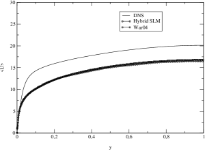
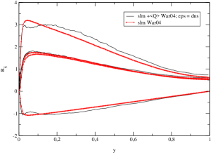
Figure 1: (a) Mean velocity Results in Wacawczyk et al. [16] (War04), in the present Hybrid configuration and in the DNS. The results are in non-dimensional units. (b) Reynolds stress results in War04 and in present Hybrid configuration, the results are in non-dimensional units.

The computations have been performed for the case of fully developed turbulent channel flow at $Re=u_{\tau}h/\nu=395$. The channel flow DNS results of Moser et al. [24] have been taken for comparison as reference data. For the simulations, the mesh used in DNS (128 points along $y$) is also used here, which assures a good interpolation of the mean fields for the Lagrangian stochastic particles. Quantities designed with the upper-script $+$ are non-dimensionalised with wall parameters. Given that the PDF used is consistent with the Eulerian Rotta Reynolds-stress model (see appendix A), this model should be used in the Eulerian part of the Hybrid method in order to check the consistency of the Lagrangian part. To ensure the best possible consistency, we use the mean fields obtained with an equivalent Lagrangian model  [16] in a stand-alone configuration. In practice, the Eulerian mean-fields computed from the Lagrangian stand-alone simulations carried on by Wacawczyk et al. [16] (designed as War04) are employed, here, as Eulerian counterpart. Indeed, the equations for the moments of first and the second order are exactly the same for both models and, thus, a perfect consistency is assured. Nevertheless, in that stand-alone calculation turbulent dissipation $\epsilon$ is not computed directly, therefore, for this variable DNS values are used and, thus, this remains a possible source of inconsistency.

In figures 1, three different profiles for the mean-velocity are shown: the profiles obtained in the stand-alone configuration in the paper of Wacawczyk et al. with an analogous viscous model, the profiles obtained in the hybrid configuration and the DNS profile, for physical reference. In figures 1, the profiles of second-order moments, that is the Reynolds stress tensor, are shown, for the present and for the War04 calculations. Generally speaking, since both methods face the same test-case, if they were completely consistent, the results would be equal both for first and second-order moments. The profiles deriving from the present PDF method are in good agreement with those computed in the stand-alone configuration. Some small differences are normal for the different numerical framework and since a different profile is used for $\epsilon$ .

Yet, in figures 1, it is possible to observe that in the zone of $y~{}\sim 0.05-0.1(y^{+}~{}\sim 10-50)$ the first components of Reynolds stress $R_{11}$ attain a nearly constant level. This merits a particular attention.

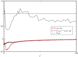
Figure 2: Comparison between dissipation and production.

This behavior can be traced back to the value of turbulent dissipation $\epsilon$ used in the present calculations. In figure 2, the dissipation and production profiles are shown as well as their ratio. It is clear that in the zone of interest a relation of equilibrium exists, the value of the ratio is near to 1 and, then, it becomes of about $0.8$ till $y^{+}~{}\sim 100$. In this range, the Reynolds-stress equations lead to the relations

$$\langle u^{2}\rangle=k\frac{C_{0}+2{\mathcal{P}}/\epsilon}{1+3C_{0}/2},\;\;k=u_{\tau}^{2}\frac{1+3C_{0}/2}{\sqrt{C_{0}}}=u_{\tau}^{2}k_{cst}~{}.$$ (96)

and, then, using the hypothesis ${\mathcal{P}}/\epsilon=1$

$$\langle u^{2}\rangle=u_{\tau}^{2}\frac{C_{0}+2}{\sqrt{C_{0}}}~{},$$ (97)

therefore, it is correct to obtain constant value of the first Reynolds stress components in the range $(y^{+}~{}\sim 10-50)$, in the present configuration.

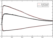
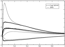
Figure 3: (a) Reynolds stress, final comparison. (b) Present results in the hybrid configurationj and DNS.

To complete our numerical validation about the consistency of the method, a slight ad-hoc modification of $\epsilon$ has been worked out. In practice, the relation between production and dissipation has been imposed to be $0.9$ in the region $y^{+}~{}\sim 10-50$, while in the rest of the domain the DNS values are maintained. In figure 3, the results are shown. The two profiles overlap. That emphasizes the consistency of the numerical method used, since the features of the Lagrangian model are perfectly reproduced. We recall that the ingredients necessary to reach this objective are:

1. Consistent physical model.

2. Consistent numerical scheme

3. Accurate global numerical method , concerning also the exchange of information from Eulerian solver to Lagrangian one.

Given that the method is found to be consistent, present calculations are also compared with DNS profiles in figure 1 and 3. From a physical point of view, the results are coherent with model features. Indeed, it is well known that the SLM model, like the Rotta RSM model, underestimates greatly the value of the components $R_{11}$ and is rather isotropic in the other diagonal components [15, 16].

5.2 Asymptotic limits

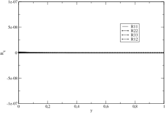
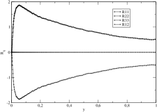
Figure 4: (a)Laminar limit case. (b) Theoretical asymptotic limit case.

A study of the numerical method in some asymptotic cases is necessary to consider the numerical validation achieved. Two cases are chosen, (a) the laminar limit case, essential in wall-bounded flows for the presence of the viscous sub-layer, and (b) a academic case where the matrix ${\bf A}$ goes to infinity, thus the time-scales $T_{1}$ and $T_{3}$ are taken to be zero, and $T_{2}=T_{L}$.

From a theoretical point of view, in these limit cases the expected behavior can be anticipated. Starting from Reynolds-stress equations, by using all hypothesis valid for the channel flow and considering the stationary case, the Reynolds-stress equations can be simplified. The equations for first, second diagonal components and for the shear stress are

$$\frac{\partial\langle v^{3}\rangle}{\partial y} = 2G_{22}\langle v^{2}\rangle+\sigma_{2}^{2},\,\,\,\quad\text{with}\,G_{22}=-1/T_{L},\quad\Rightarrow\;\langle v^{2}\rangle\approx\frac{T_{L}}{2}\sigma_{2}^{2}~{},$$ (98)

$$\frac{\partial\langle u^{2}v\rangle}{\partial y} = -2\langle uv\rangle\frac{\partial\langle U\rangle}{\partial y}+2G_{11}\langle u^{2}\rangle+2A_{12}\langle uv\rangle,\,\,\,\quad\text{with}\,G_{11}=-1/T_{1}$$ (99)

$$\frac{\partial\langle uv^{2}\rangle}{\partial y} = -2\langle v^{2}\rangle\frac{\partial\langle U\rangle}{\partial y}+2G_{11}\langle uv\rangle+2G_{22}\langle uv\rangle+2A_{12}\langle v^{2}\rangle$$ (100)

thus, as expected, in the laminar case (a) we have to find

$$T_{i}\rightarrow 0\;\Rightarrow\;R_{ij}=0~{}.$$ (101)

In the other case(b) we have

$$A_{11}=A_{33}=A_{12}\longrightarrow\infty\;\Rightarrow\;T_{1}=-\frac{1}{A_{11}}\;=\;T_{3}=-\frac{1}{A_{33}}\longrightarrow 0$$ (102)

hence, from the equations (99)-(100) we deduce

$$\langle u^{2}\rangle=-\langle uv\rangle\;,\;\langle uv\rangle=-\langle v^{2}\rangle=-\frac{T_{L}}{2}\sigma_{2}^{2}~{}.$$ (103)

The numerical results in figure 4 show that the asymptotic limits are perfectly recovered without changing time-step.

5.3 Hybrid-method error

In the last section we have studied and verified the consinstency of our hybrid method. In particular, we have checked the behaviour of the method in a theoretically consistent configuration and in the asymtotic limits. Since the consistency of the method has been successfully proofed, we can now study the global error which is eventually introduced by using an hybrid method not completely consistent. In order to better explain this very important point, let us start by considering the two phases separately.

The hybrid method for fluid-particle system exploites two different numerical (and theoretical) approaches. For fluid phase, a classical moment approach is used. This kind of algorythm is characterised by the deterministic discretisation error that is related to the numerical integration of equations in time and space. For particle phase, a Monte Carlo method is used to simulate the PDF of the stochastic process which describe particle dynamics. This method is affected both by deterministic discretization errors and, further, by the Monte Carlo error, which is related to the finite number of stochastic particles used in numerical simulations. In the stand-alone approach to stochastic equations for turbulent flows, the mean quantities present in models of form (1) are computed starting from the same stochastic particles. This procedure causes a typical Bias error which is found to be dominating in stand-alone methods [4]. In hybrid methods, this error is avoided by using a moment approach to compute the mean quantities that are necessary. In fact, this is the very strenghtness of the method. Nevertheless, even in hybrid configurations the introduction of variables computed externally may be source of errors. In particular, it is not obvious a priori what happens when the mean quantities are computed by a method which is not completely consistent with the PDF one. The error introduced by this inconsistency is intrisically inherent to the kind of hybrid method used. Moreover, from a practical point of view, the best way to investigate this effect is in a hybrid fluid-fluid configurations, where the influence of mean variables can be easily traced back.

To isolate the hybrid error, all the other errors have been made negligible in the following simulations. In both methods, a time-step of $10^{-4}$ and a spatial-step of $10^{-4}$ have been used, which can be considered as zero for our purposes. $5*10^{4}$ particles have been employed, which can be considered infinity. To the sake of clarity, the configuration discussed in last section, where stand-alone mean variables were used, it will be called standard configuration in the following.

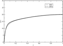
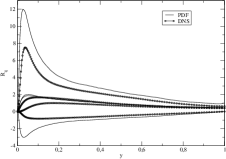
Figure 5: (a) DNS-PDF configuration: mean velocity. (b) DNS-PDF configuration: Reynolds stress.

First, we consider the following configuration: DNS results are used to provided the PDF solver with all necessary mean quantities. In figure 5, we present the mean velocity computed by the PDF method in this configuration. The DNS mean velocity is also shown as well as the mean velocity computed by PDF method in the consistent PDF-PDF configuration. The mean velocity so obtained is perfectly in agreement with DNS one and, thus, is strongly different from that obtained in the standard configuration. In fact, the exact profile is now recovered. In figure 5b, the Reynolds stress are shown for the same configuration. The profiles are dramatically changed in comparison with standard results. The $\langle uv\rangle$ and, as a consequence as we have seen, the $\langle u^{2}\rangle$ components are strongly overpredicted now. On the contrary, the other diagonal components are not changed.

This behaviour can be explained, at least approxiamatively. We have seen in the last section, analysing the behaviour in the asymptotic limits, that the diagonal $\langle v^{2}\rangle$ and $\langle w^{2}\rangle$ components are essentially dependent on Lagrangian time-scale and on diffusion coefficient, which have not changed and, therefore, they remain the same. The cross shear $\langle uv\rangle$ depends on the gradient of the mean velocity, other than on turbulent kinetic energy and on Lagrangian time-scale, thus it is much sensisitive to changes in mean velocity and, in fact, the effect of this is enourmous. Indeed, the present mean velocity profile atteins a higher maximum than in the standard configuration and, thus, it is much steeper. The shape of $\langle u^{2}\rangle$ is a direct consequence of this behaviour.

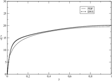
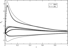
Figure 6: (a) V2F-PDF configuration: Mean velocity. (b) V2F-PDF configuration: Reynolds stress.

Now, we change again our configuration and we couple the PDF solver to a low-Reynolds number RANS model, known for his good performance in boundary flows, the v2f model [25]. In the present calculations, we use a refinement version of the model [26]. In figure 6, we show the mean velocity profile togheter with DNS and standard PDF results. As previously, the mean velocity given by our PDF method is quite near to the Eulerian mean provided to the PDF solver, in this case computed by v2f solver. Furthermore, this result is also in good agreement with DNS result. In figure 6, Reynolds stress profiles are shown. It can be seen that results are quite similar to those obtained in the DNS-PDF configuration. This time, the $<uv>$ and the $<u^{2}>$ components are less overpredicted but they show qualitatively the same behaviour.

This series of results leads us to some conclusions.

• In all three configurations tried, the mean velocity computed by stochastic particles collapses on the value of the Eulerian mean velocity that is provided by the Eulerian solver. This is in line with the physics of the model, which is basically base on a return-to-equilibrium idea [27].

• In all cases, but the standard one, there is a difference between Eulerian and Lagrangian results at the level of second-order statistical moments (Reynolds stress). This is a conseguence of coupling in a Hybrid approach two methods which are not consistent, this reasoning is valid both for PDF-DNS and for PDF-V2F configurations. Thus, it is possible to identify the global error of hybrid Eulerian/Lagrangian method by comparing the actual Reynolds stress profiles with those computed in the complete consistent configuration 3.

• In the last two configurations tried here, the results obtained are quite similar in practice, even though DNS and V2F approaches are quite different from a theoretical point of view. This is reasonable. In fact, the profiles provided by the Eulerian solver to the Lagrangian one are mean velocity, mean pressure, turbulent energy and turbulent dissipation. For these variables, the V2F approach gives results in very good agreement with DNS ones. Therefore, from the point of view of the hybrid method DNS and V2F approaches are very near. Nevertheless, the results which have been obtained using V2F are nearer to those consistent than those obtained using DNS, figure 5. Therefore, V2F model is found to be more consistent with present Lagrangian model than DNS, as expected.

The large error in the off-diagonal component of the Reynolds stress $\langle uv\rangle$ might cause some doubts about the results shown in this section. It is possible to verify by a simple numerical trick that these results could be expected.

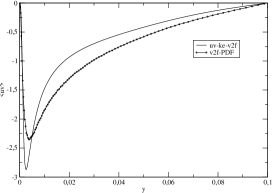
Figure 7: Reynolds stress from V2F results through $k-\epsilon$ formula.

Starting from the mean profiles obtained by the V2F approach, we can compute the $\langle uv\rangle$ component of Reynolds stress by using the $k-\epsilon$ formula

$$\langle uv\rangle=C_{\mu}\frac{k^{2}}{\epsilon}\frac{\partial\langle U\rangle}{\partial y}~{}.$$ (104)

The resulting profile is shown in figure 7 and it is compared with that obtained in the hybrid PDF-V2F configuration for the same variable. The profiles are qualitatively similar. This shows that the PDF method used is approximatetly consistent with the $k-\epsilon$, even though it is rigorously consistent with the Rotta Reynolds stress model. Furthermore, it demostrates that the difference between the V2f model and the $k-\epsilon$ model introduces an error which generates the behavior encountered for $\langle uv\rangle$.

5.4 Standard model Vs Viscous model

In this work we have proposed and tested a new Langevin viscous model for turbulent fluid flows. Other propositions have been recently made, with the aim of improving the present description of near-wall layer in the framework of PDF approach. In this section, we compare the viscous model with the standard high-Reynolds number one, in the hybrid simulation of turbulent channel flow. The high-Reynolds number model is generally used with wall-function boundary conditions, without integrating up to the wall. In the following computations, we proceed to the up-to-the-wall integration and we use the same boundary conditions imosed in the viscous case 4.

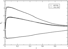
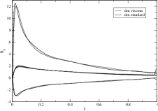
Figure 8: (a) Reynolds stress for standard and viscous model, in the consistent configuration. (b) Reynolds stress for standard and viscous model, in the DNS/PDF configuration.

First, we carry out the simulation of the channel flow in the standard consistent configuration (section 5.1). In figure 8, the Reynolds stress obtained in both cases are shown. The differences are not important, in practice, the two models give the same results. In figure 8, the Reynolds stress obtained in the hybrid DNS/PDF configuration are shown. Also in this inconsistent configuration, the results obtained with standard and viscous model do not show significant differences.

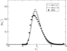
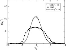
Figure 9: (a) Probability density functions computed by viscous, standard PDF and DNS approach at $y^{+}=5$. (b) Probability density functions computed by viscous, standard PDF and DNS approach at $y^{+}=10$.

In figures 9, the probability density functions of the normal velocity are shown for two locations: $y^{+}=5$ and $y^{+}=10$. The PDFs are computed with both standard and viscous PDF methods and, for reference, also DNS results are shown. Once again, the new viscous terms bring very small changes to PDF profiles. From a general point of view, it is possible to observe that in this configuration with the SLM model the PDFs remain quasi-Gaussian and the distorsion due to walls is scarcely felt, mainly in the transition zone at $y^{+}=10$. In that sense, given the good results shown by PDF methods equipped by elliptic relaxion model [28, 29], it is possible to conclude that in order to improve the quality of the physical picture the essential is given by non-local representation of pressure fluctuating term.

In conclusions, the viscous correction in near-wall models are important from a theoretical point of view, for they lead to the exact expression for first and second moment equations. However, from a practical point of view, they are negligible in hybrid configurations. Indeed, the numerical results are not influenced in a noticeable way by the viscous corrections. Other viscous models have been proposed [28, 16], but this is the first time that such comparison has been made. Moreover, the other models have been studied in stand-alone configurations, where the integration up to the wall is more delicate. Thus, it is not possible to generalize this conclusion to all PDF methods, in stand-alone methods viscous terms may be necessary in order to compute directly the near-wall zone.

6 Conclusions

First, a new physically-consistent PDF model is proposed, then, a numerical scheme for the stochastic differential equations which appear is detailed. Finally, a numerical validation of the global method is carried out with the main attention pointed on the issue of the consistency between the two approaches.

The model proposed is in the form of a set of stochastic differential equations (5)-(6). Since the model belongs to the same category of those studied previously [15, 16], a physical validation of the model, to be done necessarily with a stand-alone code, should not show particular new insights. Therefore, we suppose that the performances of the present model are equivalent to those already validated [16] and we have chosen to put the emphasis on the numerics. With regard to thos previous models, the present one is consistent with the same first and second order moment equations and thus represents just an alternative. Its main feature is that takes into account of the viscosity without changing the x-equation, as done in previous models. This presents and interest since allows a easier treatment of boundary conditions.

To simulate the stochastic process, a numerical scheme is proposed and discussed into details. This numerical scheme has been developed with some fundamental constraints in mind:

1. The numerical scheme must be explicit, uncoditionnaly stable, of order $2$ in time and the number of calls to particle localization has to be minimum.

2. The numerical scheme must be consistent with the analytical solutions of the system when the coefficients are constant.

3. The numerical scheme must be consistent with all limit systems.

These constraints are not mathematical strangeness but they come out from the intrinsic structure of the stochastic system and are important for practical concerns. Indeed, they assure consistency, accuracy and efficiency to the numerical method, even for equations which present a multi-scale character. In particular, in bounded flows velocity time-scale goes to zero with approaching to the wall and the stochastic system (15) becomes stiff. An algorithm which is not consistent with this asymptotic limit and it is not uncoditionnaly stable would require a related small integration time-step, making numerical simulations practically impossible. The consistency has been demonstrated analytically.

The numerical method obtained is validated in a Hybrid Eulerian/Lagrangian configuration. Usually a new numerical scheme is validated with a study of different errors arising from the numerical scheme, in a stand-alone configuration. Nevertheless, the problem has been analyzed exhaustively in the case of free-shear fluid flows with another weak second-order scheme [4] and in the case of two-phase flows for an analogous scheme [14]. In particular, the last scheme is retrieved rigorously by the present scheme in the case of high Reynolds-number flows (when viscosity is put to zero). Thus, we have preferred to concentrate ourselves on the major point of the consistency of the hybrid Eulerian/Lagrangian method, which is a fundamental issue for this kind of approach [7]. The global method is found to be perfectly consistent at the level of first two velocity moments. Moreover, analytical results for Reynolds stress are recovered in the asymptotic limits, which supports also the numerical validation of the numerical scheme.

In this numerical validation, it has been pointed out two other main points: (i) Eulerian/Lagrangian methods which are not consistent with the same turbulence model like DNS/SLM or V2F/SLM suffer from an important bias error which make result flawed. Therefore such configurations often proposed in two-phase flows should reconsidered critically. (ii) It has been shown that in a hybrid framework the viscous and non-viscous models give basically the same results, provided the correct boundary conditions are imposed.

Finally, the main point to underline, about the development of the numerical scheme, is that the methodology presented goes beyond the borders of the present model and of present calculations. The main objective was to propose a safe guideline to follow, when one has to deal with numerical simulations of stochastic models. Moreover, the methodology is not restricted to fluid mechanical applications, but it can be applied without modifications to whatever model which has a form of linear SDEs, for example in polymeric fluids [1].

Appendix A Properties of the physical model

The mean momentum equation is simply obtained by applying the averaging operator to the particle velocity equation (6)

$$\langle dU_{i}\rangle=-\frac{1}{\rho}\frac{\partial\langle P\rangle}{\partial x_{i}}\,dt+\nu\frac{\partial^{2}\langle U_{i}\rangle}{\partial x_{k}^{2}}.$$ (A.1)

Using the relation between the instantaneous substantial derivative and its Eulerian counterpart, $d\cdot/dt=\partial\cdot/\partial t+U_{j}\partial\cdot/\partial x_{j}$, we obtain

$$\frac{\partial\langle U_{i}\rangle}{\partial t}+\langle U_{j}\rangle\frac{\partial\langle U_{i}\rangle}{\partial x_{j}}+\frac{\partial\langle u_{i}u_{j}\rangle}{\partial x_{j}}=-\frac{1}{\rho}\frac{\partial\langle P\rangle}{\partial x_{i}}+\nu\frac{\partial^{2}\langle U_{i}\rangle}{\partial x_{k}^{2}}.$$ (A.2)

Thus, the exact mean Navier-Stokes equation is satisfied. This should not be too surprising since convection is treated without approximation by the Lagrangian point of view and since the mean pressure-gradient, which represents the mean value of the acceleration of a fluid particle, is properly taken into account in Eq. (6). For the second order, one has to write the instantaneous equations for the fluctuating velocity components along a particle trajectory. This is done by writing $u_{i}=U_{i}-\langle U_{i}\rangle$ and consequently

$$\frac{du_{i}}{dt}=\frac{dU_{i}}{dt}-\left\{\frac{\partial\langle U_{i}\rangle}{\partial t}+\langle U_{j}\rangle\frac{\partial\langle U_{i}\rangle}{\partial x_{j}}\right\}-u_{j}\frac{\partial\langle U_{i}\rangle}{\partial x_{j}}.$$ (A.3)

We now write the equation in an incremental form to properly handle the stochastic terms, which using the mean Navier-Stokes equation is

$$du_{i}=\frac{\partial\langle u_{i}u_{k}\rangle}{\partial x_{k}}\,dt-u_{k}\frac{\partial\langle U_{i}\rangle}{\partial x_{k}}\,dt+G_{ik}u_{k}\,dt+A_{ik}u_{k}\,dt+\sqrt{C_{0}\langle\epsilon\rangle}dW_{i}.$$ (A.4)

The first two terms on the rhs are exact and are independent of the form of the stochastic model. The different SDEs are defined in the Itô sense and the derivatives of the products $u_{i}u_{j}$ are obtained from Itô’s formula

$$d(u_{i}u_{j})=u_{i}du_{j}+u_{j}du_{i}+C_{0}\langle\epsilon\rangle\,dt\delta_{ij}.$$ (A.5)

The mean second-order equations are then

$$\begin{split}\frac{\partial\langle u_{i}u_{j}\rangle}{\partial t}+\langle U_{k}\rangle\frac{\partial\langle u_{i}u_{j}\rangle}{\partial x_{k}}+\frac{\partial\langle u_{i}u_{j}u_{k}\rangle}{\partial x_{k}}=&-\langle u_{i}u_{k}\rangle\frac{\partial\langle U_{j}\rangle}{\partial x_{k}}-\langle u_{j}u_{k}\rangle\frac{\partial\langle U_{i}\rangle}{\partial x_{k}}\\ &+G_{ik}\langle u_{j}u_{k}\rangle+G_{jk}\langle u_{i}u_{k}\rangle\\ &+\nu\frac{\partial\langle u_{i}u_{j}\rangle}{\partial x_{k}^{2}}+C_{0}\langle\epsilon\rangle\delta_{ij}.\end{split}$$ (A.6)

Appendix B Calculus of the stochastic integrals

Here, it is explained how the stochastic integrals, appearing in the analytical solutions of the equation system with constant coefficients, can be re-arranged (by stochastic integration by parts), to yield the covariance matrix.

B.1 Integration by parts

Let $X(t)$ and $Y(t)$ be two diffusion processes. One can show that (see for example Klebaner [12]), in the Itô sense,

$$X(t)Y(t)-X(t_{0})Y(t_{0})=\int_{t_{0}}^{t}X(s)\,dY(s)+\int_{t_{0}}^{t}Y(s)\,dX(s)+[X,Y](t),$$

where $[X,Y](t)$ is the quadratic covariation of $X(t)$ and $Y(t)$ on $[t_{0},t]$. In the case where one of the processes is deterministic, $[X,Y](t)=0$. In the frame of our study, where the integrated variable is always a deterministic function, one can therefore apply integration by parts as in classical differential calculus.

In fact, in the analytical solutions of the equation system with constant coefficients, one encounters multiple stochastic integrals of the type

$$I=\int_{t_{0}}^{t}\exp(-s/a)\left(\int_{t_{0}}^{s}\exp(s^{\prime}/b)\,dW(s^{\prime})\right)\,ds,$$ (B.1)

where $(a,b)\in\mathbb{R}^{+2}$. By setting

$$F(s)=\int_{t_{0}}^{s}\exp(s^{\prime}/b)\,dW(s^{\prime})\,\Longrightarrow\,dF(s)=\exp(s/b)\,dW(s),$$

$$dG(s)=\exp(-s/a)\,\Longrightarrow\,G(s)=-a\,\exp(-s/a)\,ds,$$

and applying integration by parts, one obtains

$$I=-a\,\exp(-t/a)\int_{t_{0}}^{t}\exp(s/b)\,dW(s)+a\int_{t_{0}}^{t}\exp(-s/a)\,\exp(s/b)\,dW(s).$$ (B.2)

Therefore, by stochastic integration by parts, the multiple integral given by Eq. (B.1) can be written as the sum of two simple stochastic integrals, Eq. (B.2).

B.2 Derivation of the covariance matrix

By using the results of the previous subsection and the main properties of the Itô integral, that is, linearity, the zero mean property,

$$\langle\int_{t_{0}}^{t}X(s)\,dW(s)\rangle=0,$$

and the isometry property,

$$\langle\int_{t_{0}}^{t_{1}}X(s)\,dW(s)\int_{t_{2}}^{t_{3}}Y(s)\,dW(s)\rangle=\int_{t_{2}}^{t_{1}}\langle X(s)Y(s)\rangle\,ds,$$

with $t_{0}<t_{2}<t_{1}<t_{3}$. From the zero mean property, it follows that the first order moments are equal to zero. For the second order moments (covariance matrix), the previous properties give the following equality

$$\begin{split}\langle\left(\sum_{m}g_{m}(t)\int_{t_{0}}^{t}f_{m}(s)\,dW(s)\right)^{2}\rangle&=\\ \sum_{m}g^{2}_{m}(t)&\int_{t_{0}}^{t}f^{2}_{m}(s)\,ds+2\sum_{m<k}g_{m}(t)\,g_{k}(t)\int_{t_{0}}^{t}f_{m}(s)\,f_{k}(s)\,ds.\end{split}$$ (B.3)

where $g_{im}(t)$ and $f_{im}(t)$ are deterministic functions of time.

Appendix C Simulation of a Gaussian vector

Let ${\mathbf{X}}=(X_{1},\dots,X_{d})$ be a Gaussian vector defined by a zero mean and a covariance matrix $C_{ij}=\langle X_{i}X_{j}\rangle$. For all positive symmetric matrix (such as $C_{ij}$), there exists a (low or high) triangular matrix $P_{ij}$ which verifies

$${\mathbf{C}}={\mathbf{P}}{\mathbf{P}}^{t}\,\Longrightarrow\,C_{ij}=\sum_{k=1}^{d}P_{ik}P_{jk}.$$

${\mathbf{P}}$ is given by the Choleski algorithm (here for the low triangular matrix)

$$\begin{split}&P_{i1}=\frac{C_{i1}}{\sqrt{(}C_{11})},\quad 1\leqslant i\leqslant d\\ &P_{ii}=\left(C_{ii}-\sum_{j=1}^{i-1}P_{ij}\right)^{1/2},\quad 1<i\leqslant d\\ &P_{ij}=\frac{1}{P_{jj}}\left(C_{ij}-\sum_{k=1}^{j-1}P_{ik}P_{jk}\right),\quad 1<j<i\leqslant d\\ &P_{ij}=0,\quad i<j\leqslant d.\end{split}$$

Let ${\mathbf{G}}=(G_{1},\dots,G_{d})$ be a vector composed of independent $\mathcal{N}(0,1)$ Gaussian random variables, then it can be shown that the vector ${\mathbf{Y}}={\mathbf{P}}{\mathbf{G}}$ is a Gaussian vector of zero mean and whose covariance matrix is ${\mathbf{C}}={\mathbf{P}}{\mathbf{P}}^{t}$. Therefore, ${\mathbf{X}}$ and ${\mathbf{Y}}$ are identical, that is,

$${\mathbf{X}}={\mathbf{P}}{\mathbf{G}}\,\Longrightarrow\,X_{i}=\sum_{k=1}^{d}P_{ik}G_{k}.$$ (C.1)

Eq. (C.1) shows how the stochastic integrals, obtained in the analytical solutions of the system with constant coefficients, can be simulated.

References

• [1] H. C. Öttinger. Stochastic Processes in Polymeric Fluids. Tools and Examples for Developing Simulation Algorithms. Springer, Berlin, 1996.
• [2] S. B. Pope. Pdf methods for turbulent reactive flows. Prog. Energy Combust. Sci., 11:119–192, 1985.
• [3] J-P. Minier and E. Peirano. The pdf approach to polydispersed turbulent two-phase flows. Physics Reports, 352(1–3):1–214, 2001.
• [4] Xu J. and Pope S.B. Assessment of numerical accurary of pdf/monte carlo methods for turbulent reacting flows. J. Comput. Phys., 152:192, 1999.
• [5] R. W. Hockney and J. W. Eastwood. Computer simulations using particles. Institute of Physics Publishing, Bristol and Philadelphia, 1988.
• [6] G. Bird. Molecular Gas Dynamics and the Direct Simulation of Gas Flows. Clarendon Press, Oxford, 1994, 1994.
• [7] M Muradoglu, SB Pope, and DA Caughey. The hybrid method for the pdf equations of turbulent reactive flows: consistency conditions and correction algorithms. Journal of Computational Physics, 172(2):841–878, 2001.
• [8] E. Peirano, S. Chibbaro, J. Pozorski, and J.-P. Minier. Mean-field/pdf numerical approach for polydispersed turbulent two-phase flows. Prog. En. Comb. Sci., 32(3):315, 2006.
• [9] W.C. Welton. Two-dimensional pdf/sph simulations of compressible turbulent flows. J. Comput. Phys., 139:410–443, 1998.
• [10] L.Y.M. Gicquel, P. Givi, F.A. Jaberi, and S. B. Pope. Velocity filtered density function for large eddy simulation of turbulent flows. Phys. Fluids, 14:1196, 2002.
• [11] Sergio Chibbaro and Jean-Pierre Minier. A note on the consistency of hybrid eulerian/lagrangian approach to multiphase flows. arXiv, physics.flu-dyn, Dec 2009. 14 pages, 3 figures.
• [12] F. C. Klebaner. Introduction to stochastic calculus with applications. Imperial College Press, London, 1999.
• [13] J-P. Minier. Probabilistic approach to turbulent two-phase flows modelling and simulation: theoretical and numerical issues. Monte Carlo Methods and Appl., 7(3–4):295–310, 2000.
• [14] J-P. Minier, E. Peirano, and S. Chibbaro. Weak first- and second order numerical schemes for stochastic differential equations appearing in lagrangian two-phase flow modelling. Monte Carlo Meth. and Appl., 9(2):93, 2003.
• [15] T. D. Dreeben and S. B. Pope. Probability density function and reynolds-stress modeling of new near-wall turbulent flows. Phys. Fluids, 9:154, 1997.
• [16] M. Waclawczyk, J. Pozorski, and J-P. Minier. Probablility density function computation of turbulent flows with a new near-wall model. Phys. Fluids, 16(5):1410, 2004.
• [17] S Chibbaro and J Minier. Langevin pdf simulation of particle deposition in a turbulent pipe flow. Journal of Aerosol Science, Jan 2008.
• [18] P.E. Kloeden and E. Platen. Numerical solution of stochastic differential equations. Springer-Verlag, Berlin, 1992.
• [19] D. Talay. Simulation of Stochastic Differential Equation, in Probabilistic Methods in Applied Physics. Springer-Verlag, Berlin, 1995.
• [20] J-P. Minier, R. Cao, and S. B. Pope. Comment on the article "an effective particle tracking scheme on structured/unstructured grids in hybrid finite volume/pdf monte carlo methods" by li and modest. J. Compt. Phys., 186:356–358, 2003.
• [21] S. B. Pope. Lagrangian pdf methods for turbulent reactive flows. Annu. Rev. Fluid Mech., 26:23–63, 1994.
• [22] R. Garg, C. Narayanan, D. Lakehal, and S. Subramaniam. Accurate numerical estimation of interphase momentum transfer in lagrangian–eulerian simulations of dispersed two-phase flows. Int. Journal Multiphase flows, 33:1337, 2007.
• [23] R. Garg, C. Narayanan, , and S. Subramaniam. A numerically convergent lagrangian–eulerian simulation method for dispersed two-phase flows. Int. Journal Multiphase flows, 35:376, 2009.
• [24] P. Moser, Kim J., and N. N. Mansour. Direct numerical simulation of turbulent channel flow up to retau = 590. Phys. Fluids, 11:943, 1999.
• [25] P.A. Durbin. Near-wall turbulence closure modeling without damping functions. Theor. Comput. Fluid Dyn, 3:1–13, 1991.
• [26] Laurence D. R., Uribe J.C., and Utyuzhnikov S.V. A robust formulation of the v2-f model. Flow, Turbulence and Combustion, 73:169, 2005.
• [27] J-P. Minier and J. Pozorski. Derivation of a pdf model for turbulent flows based on principles from statistical physics. Phys. Fluids, 9(6):1748–1753, 1997.
• [28] T. D. Dreeben and S. B. Pope. Probability density function/monte carlo simulation of near-wall turbulent flows. J. Fluid Mech., 357:141, 1998.
• [29] J. Pozorski, M. Waclawczyk, and J-P. Minier. Scalar and joint velocity-scalar pdf modeling of near-wall turbulent heat transfer. Int. J. Heat and Fluid Flow, 25:884–895, 2004.