NLO and Parton Showers: the POWHEG-BOX

Abstract

We describe the POWHEG-BOX package, a general computer code framework for implementing NLO calculations in Shower Monte Carlo programs according to the POWHEG method.

1 The POWHEG method

Next-to-leading order (NLO) perturbative QCD computations as well as Shower Monte Carlo (SMC) programs are fundamental tools for the present-days particle physics phenomenology. In particular, SMC programs incorporate the description of a generic high-energy hadronic collision process, starting from the collision between constituents and developing the parton shower, that increases the number of final-state particles by means of strongly ordered subsequent emissions. Eventually, the interface with a phenomenological hadronization model, enables the comparison with experimental data. For these reasons, they are routinely used by experimentalists to simulate signal and backgrounds processes in physics searches. Nevertheless, the demand for better and better predictions from high energy experiments calls for improving the precision of existing SMC’s, including NLO corrections. The MC@NLO [1] method has shown first how to reach NLO accuracy for inclusive quantities, implementing the hard subprocess at NLO and developing showers within the leading logarithmic approximation, avoiding double counting of radiation. In this way one achieves benefits of both approaches: exclusive final states generation of SMC’s and accuracy of NLO calculations.

The POWHEG method is a different prescription for interfacing NLO calculations with parton shower generators. It was first suggested in ref. [2], and was described in great detail in ref. [3]. This method is independent from the Monte Carlo program used for subsequent showering and generates positive weighted events only. In these respects it improves the MC@NLO approach. Until now, the POWHEG method has been successfully applied to several processes, both at lepton [4, 5] and hadron colliders [6, 7, 8, 9, 10, 11, 12, 13, 14]. In these implementations, it has been interfaced to the HERWIG [15, 16], PYTHIA [17] and HERWIG++ [18] SMC programs.

In the POWHEG method the hardest radiation is generated first, independently from the following ones. Schematically, the hardest radiation is distributed according to

$$d\sigma=\bar{B}\left(\Phi_{B}\right)\,d\Phi_{B}\,\left[\Delta_{R}\left(p_{T}^{\min}\right)+\frac{R\left(\Phi_{R}\right)}{B\left(\Phi_{B}\right)}\,\Delta_{R}\left(k_{T}\left(\Phi_{R}\right)\right)\,d\Phi_{\mathrm{rad}}\right]\,,$$ (1)

where $B\left(\Phi_{B}\right)$ is the Born contribution and

$$\bar{B}\left(\Phi_{B}\right)=B\left(\Phi_{B}\right)+\left[V\left(\Phi_{B}\right)+\int d\Phi_{\mathrm{rad}}\,R\left(\Phi_{R}\right)\right]$$ (2)

is the NLO differential cross section at fixed underlying Born kinematics and integrated over the radiation variables. The transverse momentum of the emitted parton, with respect to the beam or to another particle, depending on the region of singularity, is denoted by $k_{T}\left(\Phi_{R}\right)$. The lower cutoff $p_{T}^{\min}$ is necessary in order to avoid the coupling constant to reach unphysical values. $V\left(\Phi_{B}\right)$ and $R\left(\Phi_{R}\right)$ are the virtual and the real corrections and in the expression within the square bracket in Eq. (2) a procedure that takes care of the cancellation of soft and collinear singularities is understood, e.g. Frixione-Kunszt-Signer (FKS) [19] or Catani-Seymour (CS) dipole subtraction. Then,

$$\Delta_{R}\left(p_{T}\right)=\exp\left[-\int d\Phi_{\mathrm{rad}}\,\frac{R\left(\Phi_{R}\right)}{B\left(\Phi_{B}\right)}\,\theta\left(k_{T}\left(\Phi_{R}\right)-p_{T}\right)\right]\,$$ (3)

is the POWHEG Sudakov, that is the probability of not having an emission harder that $p_{T}$. Equation (1) can be seen as an improvement on the original SMC hardest-emission formula, since the Born cross section is replaced with $\bar{B}\left(\Phi_{B}\right)$ which is normalized to NLO by construction. At small transverse momenta the POWHEG Sudakov becomes equal to a standard SMC one. However, the NLO accuracy of Eq. (1) is maintained for inclusive quantities. Moreover, the high$-p_{T}$ radiation region is correctly described by the real contributions

$$d\sigma\approx\bar{B}\left(\Phi_{B}\right)\,d\Phi_{B}\,\frac{R\left(\Phi_{R}\right)}{B\left(\Phi_{B}\right)}d\Phi_{\mathrm{rad}}\ \approx R\left(\Phi_{R}\right)d\Phi_{B}d\Phi_{\mathrm{rad}}\,,$$ (4)

since $\Delta_{R}\approx 1$ and $\bar{B}/B\approx 1+\mathcal{O}\left({\alpha_{\scriptstyle{\rm s}}}\right)$. After having generated the hardest radiation, one can interface with any available shower generator, in order to develop the rest of the shower. To avoid the double-counting, the SMC is required to be either $p_{T}-$ordered or to have the ability to veto emissions with a $p_{T}$ harder than the first one.

2 The POWHEG-BOX

In a real collision process several colored massless partons are present, either in the initial or the final state. One thus should repeat the procedure outlined in Sec. 1 for every possible singular region, associated with any massless colored leg becoming collinear to another one, or soft. In order to do this, the full real emission cross section is decomposed into a sum of terms, each of which has at most one collinear and one soft singularities. The radiation is then generated independently in each of this regions, but only the hardest radiation is retained and the event is generated according to the flavour and kinematics associated to it. Because of this complexity, an automatic tool, the POWHEG-BOX, has been built [21], in order to help the inclusion of new processes. On the other hand, the POWHEG-BOX may also be seen as a library, where previously implemented processes are available in a common framework.

The user wishing to include a new NLO calculation must only know how to communicate the needed information to the POWHEG-BOX. This happens either defining the appropriate variables, either providing the necessary Fortran routines. The required inputs are:

1. The number of legs in Born process, e.g. nlegborn$=5$ for $pp\to(Z\to e^{+}e^{-})+j$.

2. The list of Born and Real processes flavours flst_born(k=1..nlegborn,j=1..flst_nborn), flst_real(k=1..nlegreal,j=1..flst_nreal), according to PDG [22] conventions. Flavor is defined incoming (outgoing) for incoming (outgoing) fermion lines, e.g. [5,2,23,6,3,0] for $bu\ \to\ Ztsg$.

3. The Born phase space Born_phsp(xborn), given xborn(1...ndims) random numbers in the unit ndims-dimensional hypercube. This routine should also set the Born phase space Jacobian kn_jacborn, the Born momenta kn_pborn, kn_cmpborn in lab. and CM frames and the Bjorken $x$’s, i.e. kn_xb1,kn_xb2 .

4. The routines that performs the initialization of the couplings, init_couplings, and the setting of the factorization and renormalization scales, set_fac_ren_scales(muf,mur).

5. The Born squared amplitudes ${\cal B}=|{\cal M}|^{2}$, summed and averaged over color and helicities as well as the color-ordered Born squared amplitudes ${\cal B}_{jk}$ and the helicity correlated Born squared amplitudes ${\cal B}_{k,\mu\nu}$, where $k$ runs over all external gluons. The corresponding user routine is defined by setborn(p,bflav,born,bornjk,bornmunu), for momenta p(0:3,1:nlegborn) and flavour string bflav(1:nlegborn) .

6. The real emission squared amplitudes ${\cal R}$ user routine setreal(p,rflav,amp2), for momenta p(0:3,1:nlegreal) and flavour string rflav(1:nlegreal) .

7. The finite part of the interference of Born and virtual amplitude contributions ${\cal V}_{\rm b}=2\mathrm{Re}\{{\cal B}\times{\cal V}\}$, after factorizing out the common factor $\mathcal{N}=\frac{(4\pi)^{\epsilon}}{\Gamma\left(1-\epsilon\right)}\left(\frac{\mu_{\mathchoice{\displaystyle}{\scriptstyle}{\scriptscriptstyle}{\scriptscriptstyle}\rm R}^{2}}{Q^{2}}\right)^{\epsilon}$. The user routine is called setvirtual(p(0:3,1:nlegborn),vflav(1:legborn),virtual).

8. The Born color structures in the large $N_{\rm c}$ limit, set by the routine borncolour_lh and passed through the Les Houches interface [20].

We remark that items (1-7) are the usual ingredients needed to perform a NLO calculation in any subtraction method. Item (8) is instead needed to provide a defined color structure to the SMC generator. Internally, the POWHEG-BOX implements the FKS subtraction procedure in a general way. At the beginning, it automatically evaluates the combinatorics, identifying all the singular regions and the corresponding underlying Born contributions. It also performs the projection of real contributions over the singular region and computes the subtraction counterterms, from soft and collinear approximations of real emissions. Then, it builds the ISR and FSR phase space, according to the FKS parametrization of the singular region and performs the integration. Eventually, one gets the NLO differential cross section. At this stage, one can also interface to some analysis routine to obtain NLO differential distributions as a byproduct. After the integration stage, it performs the calculation of upper bounds for an efficient generation of Sudakov-suppressed events and then the generation of hardest radiation, according to the POWHEG Sudakov. At this point, the generated event, which contains at most only one extra radiation, has to be passed to a standard SMC program, for developing the rest of the shower. This can be done either on-the-fly or storing the events on a Les Houches events file [23]. Standard analysis routines, at partonic and hadronic level, are provided for included processes, as well as drivers for common SMC generators. Users can modify them or implement new ones.

2.1 Recent developments

Recently, thanks to this framework, the relatively complex process of $Z+1\ jet$ production has been implemented [24]. This is a promising processes for jet calibration with the early LHC data. It is also an important source of missing energy signal as well as a background to many new physics searches. In experimental studies carried up until now, the NLO theoretical calculations were supplemented by correction factors for shower, hadronization and underlying event effects. However, these factors were evaluated by means of standard LO SMC programs. It is clear the advantage to have a SMC program which is NLO accurate, in order to ease and improve the comparisons with experimental results. We have tried a simple approach [24] to merge consistently $Z$ and $Z+1\ jet$ samples, in order to obtain a description as smooth and accurate as possible both in the low and high-transverse momentum regions. The results are showed in Figs. 2 and 2.

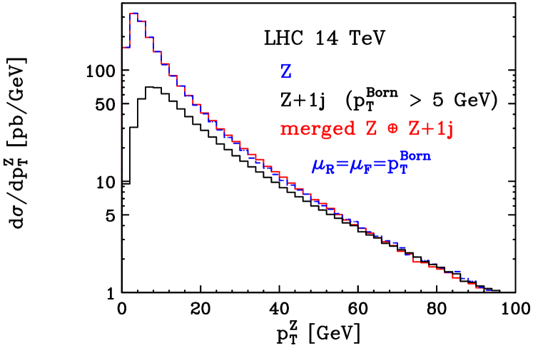
Figure 1: The $p_{T}$ distribution of the $Z$ boson in single $Z$ production (blue dashed curve), in $Z+1$ jet (black solid) and in the merged sample (red solid).

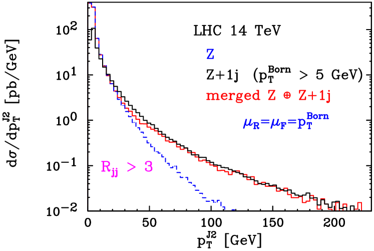
Figure 2: The $p_{T}$ distribution of the next-to-hardest jet in single $Z$ production (blue dashed curve), in $Z+1$ jet (black solid) and in the merged sample (red solid).

From the two figures, one can see how the merged sample models both the single $Z$ Sudakov form factor, that plays an important role in resumming collinear/soft logarithms in the low-$p_{T}$ region and the high-$p_{T}$ behaviour of the next-to-hardest jet, which follows the $Z+1$ jet distribution. In this last figure, jest are reconstructed according to the $k_{T}$ algorithm, imposing also an angular separation $R_{jj}>3$ .

References

- [1] S. Frixione and B. R. Webber, JHEP 0206 (2002) 029 [arXiv:hep-ph/0204244].
- [2] P. Nason, JHEP 0411 (2004) 040 [arXiv:hep-ph/0409146].
- [3] S. Frixione, P. Nason and C. Oleari, JHEP 0711 (2007) 070 [arXiv:0709.2092 [hep-ph]].
- [4] O. Latunde-Dada, S. Gieseke and B. Webber, JHEP 0702 (2007) 051 [arXiv:hep-ph/0612281].
- [5] O. Latunde-Dada, Eur. Phys. J. C 58 (2008) 543 [arXiv:0806.4560 [hep-ph]].
- [6] P. Nason and G. Ridolfi, JHEP 0608 (2006) 077 [arXiv:hep-ph/0606275].
- [7] S. Frixione, P. Nason and G. Ridolfi, JHEP 0709 (2007) 126 [arXiv:0707.3088 [hep-ph]].
- [8] S. Alioli, P. Nason, C. Oleari and E. Re, JHEP 0807 (2008) 060 [arXiv:0805.4802 [hep-ph]].
- [9] K. Hamilton, P. Richardson and J. Tully, JHEP 0810 (2008) 015 [arXiv:0806.0290 [hep-ph]].
- [10] A. Papaefstathiou and O. Latunde-Dada, JHEP 0907 (2009) 044 [arXiv:0901.3685 [hep-ph]].
- [11] S. Alioli, P. Nason, C. Oleari and E. Re, JHEP 0904 (2009) 002 [arXiv:0812.0578 [hep-ph]].
- [12] K. Hamilton, P. Richardson and J. Tully, JHEP 0904 (2009) 116 [arXiv:0903.4345 [hep-ph]].
- [13] S. Alioli, P. Nason, C. Oleari and E. Re, JHEP 0909 (2009) 111 [Erratum-ibid. 1002 (2010) 011] [arXiv:0907.4076 [hep-ph]].
- [14] P. Nason and C. Oleari, JHEP 1002 (2010) 037 [arXiv:0911.5299 [hep-ph]].
- [15] G. Corcella et al., JHEP 0101 (2001) 010 [arXiv:hep-ph/0011363].
- [16] G. Corcella et al., arXiv:hep-ph/0210213.
- [17] T. Sjostrand, S. Mrenna and P. Z. Skands, JHEP 0605 (2006) 026 [arXiv:hep-ph/0603175].
- [18] M. Bahr et al., Eur. Phys. J. C 58, 639 (2008) [arXiv:0803.0883 [hep-ph]].
- [19] S. Frixione, Z. Kunszt and A. Signer, Nucl. Phys. B 467 (1996) 399 [arXiv:hep-ph/9512328].
- [20] E. Boos et al., arXiv:hep-ph/0109068.
- [21] S. Alioli, P. Nason, C. Oleari and E. Re, JHEP 1006 (2010) 043 [arXiv:1002.2581 [hep-ph]].
- [22] http://pdg.lbl.gov
- [23] J. Alwall et al., Comput. Phys. Commun. 176 (2007) 300 [arXiv:hep-ph/0609017].
- [24] S. Alioli, P. Nason, C. Oleari, and E. Re, In preparation.