Helical spin textures in dipolar Bose–Einstein condensates

Abstract

We numerically study elongated helical spin textures in ferromagnetic spin-1 Bose–Einstein condensates subject to dipolar interparticle forces. Stationary states of the Gross–Pitaevskii equation are solved and analyzed for various values of the helical wave vector and dipolar coupling strength. We find two helical spin textures which differ by the nature of their topological defects. The spin structure hosting a pair of Mermin–Ho vortices with opposite mass flows and aligned spin currents is stabilized for a nonzero value of the helical wave vector.

I Introduction

Helical structures lie at the heart of several feats of innovation. The Archimedean screw and spiral staircases are inventions dating back to ancient history. Simple bolts and spring coils stand as hallmarks of practicality in modern everyday life. Helical growth is a clear demonstration that such structures also exist naturally without human intervention. On the other hand, helices are vital for life itself as we know it, the DNA polymer being a famous example of a double-helix structure Watson1953 .

The study of helical spin textures has recently drawn attention in the field of gaseous spinor Bose–Einstein condensates (BECs). In a quantum degenerate gas of ferromagnetic spin-1 ${}^{87}{\rm Rb}$, a helical magnetization texture was observed to decay into small spin domains Vengalattore2008 . This effect was argued to result from the weak interatomic magnetic dipole forces in the system. Closely related to the experiment, the dynamical instability of an $XY$ spiral state has been investigated theoretically Cherng2008 .

It has been predicted that a sufficiently strong magnetic dipolar forces can spontaneously give rise to intriguing spin textures in ferromagnetic condensates: the long-range dipolar potential stabilizes spin-vortex states in various geometries, as was demonstrated using a spin-1 model Yi2006 ; Kawaguchi2006 and a classical spin approach Takahashi2007 ; Huhtamaki2010 . Even weak dipolar interactions can lead to dynamic formation of a helical spin texture in a ferromagnetic spin-1 BEC Kawaguchi2007 . In the absence of external magnetic fields, the spin helix can appear as the ground-state texture in a suitable geometry and with strong enough dipolar interactions Huhtamaki2010 .

In the present article, we investigate helical spin textures in ferromagnetic dipolar condensates using a spin-1 model. We find stationary helical states under the assumption that the system is infinitely long in the direction of the helix axis and find solutions hosting different types of topological line defects, i.e., quantized vortices. Due to the symmetry of the order-parameter field, these line defects encircle the condensate in a helical pattern. The resulting vortex structure resembles a pair of vortices excited in Kelvin modes in a stationary configuration. Direct experimental evidence of Kelvin waves has been observed in a spin-polarized BEC of ${}^{87}{\rm Rb}$ by studying two transverse quandrupole modes of the atomic cloud Bretin2003 . Kelvin-wave excitations of quantized vortices have also been studied theoretically in a similar setup Mizushima2003 ; Fetter2004 ; Simula2008 . Moreover, helical vortices in a two-component condensate have been investigated Cho2005 .

Although we focus on a spin-1 BEC, the study can also shed light on phenomena in strongly dipolar systems with more complex order parameters. The energy-minimizing helical spin textures that we obtain are in qualitative agreement with those found earlier using the classical spin approach Huhtamaki2010 . Since the classical spin model is supposed to be accurate for ferromagnetic systems in the limit of large magnetic moments, it is plausible to expect that similar structures exist independent of the value of the atomic spin number $F$. The most timely example of a condensate with larger $F$ and significant dipolar interactions is the spin-3 gas of ${}^{52}{\rm Cr}$ Griesmaier2005 which has been produced by purely optical means Beaufils2008 . The chromium atoms have magnetic moments of $6\,\mu_{\mathrm{B}}$, whereas the maximal atomic magnetic moment for an alkali-metal condensate is $1\,\mu_{\mathrm{B}}$. Recently, there has been progress in cooling and trapping vapors of $\mathrm{Tm}$ $(4\,\mu_{\mathrm{B}})$ Sukachev2010 , $\mathrm{Er}$ $(7\,\mu_{\mathrm{B}})$ Berglund2008 , and $\mathrm{Dy}$ $(10\,\mu_{\mathrm{B}})$ Lu2010 , the last having the largest atomic magnetic moment of all known elements.

II Theory

In this work, we study ferromagnetic spin-1 BECs, such as ${}^{87}{\rm Rb}$, using a zero-temperature mean-field model. In addition to the density–density and spin–spin interatomic forces, we also include long-range dipolar interactions in the model.

Stationary states of the system are solutions to the time-independent Gross–Pitaevskii (GP) equation

$$\hat{h}\Psi({\bf r}) + gn({\bf r})\Psi({\bf r})+g_{\mathrm{s}}\sum_{\alpha}M_{\alpha}({\bf r})\hat{S}_{\alpha}\Psi({\bf r})$$

$$+ g_{\mathrm{d}}\sum_{\alpha,\beta}\int d^{3}r^{\prime}D_{\alpha\beta}({\bf r}-{\bf r}^{\prime})M_{\alpha}({\bf r}^{\prime})\hat{S}_{\beta}\Psi({\bf r})=0,$$

where $\Psi=\left(\psi_{1},\psi_{0},\psi_{-1}\right)^{T}$ is a three-component spinor order parameter, $\hat{h}=-\hbar^{2}\nabla^{2}/2m+V_{\rm trap}({\bf r})-\mu$ is the single-particle Hamiltonian, and $\hat{S}_{\alpha}$ denotes the $\alpha$th component of the dimensionless $F=1$ spin operator whose spin-space expectation value gives the $\alpha$th component of magnetization, $M_{\alpha}({\bf r})=\Psi^{\dagger}({\bf r})\hat{S}_{\alpha}\Psi({\bf r})$. The density of particles is given by $n({\bf r})=\sum\psi_{k}^{*}({\bf r})\psi_{k}({\bf r})$, where the components $\left(\psi_{1},\psi_{0},\psi_{-1}\right)$ are the projections of $\Psi$ onto the eigenbasis of $\hat{S}_{z}$. The total number of particles per unit length, $\int d^{2}r\,n({\bf r})=N$, is controlled through the chemical potential $\mu$ acting as a Lagrange multiplier.

The coupling constants $g$, $g_{\mathrm{s}}$ and $g_{\mathrm{d}}$ measure the strengths of the local density–density, local spin–spin, and non-local magnetic dipole–dipole interactions, respectively. The first two are related to the scattering lengths $a_{0}$ and $a_{2}$ into spin channels with total spin $0$ and $2\hbar$ through $g=4\pi\hbar^{2}(a_{0}+2a_{2})/3m$ and $g_{\mathrm{s}}=4\pi\hbar^{2}(a_{2}-a_{0})/3m$. Throughout the work, we use $g_{\mathrm{s}}=-0.01\,g$, which is roughly the coupling constant for ${}^{87}{\rm Rb}$ Klausen2001 ; Kempen2002 ; Widera2006 and a value previously used, e.g., in Yi2006 ; Simula2010 . The dipolar coupling constant is given by $g_{\mathrm{d}}=\mu_{0}\mu_{\mathrm{B}}^{2}g_{\mathrm{F}}^{2}/4\pi$ with $\mu_{0}$, $\mu_{\mathrm{B}}$, and $g_{\mathrm{F}}$ being the permeability of vacuum, the Bohr magneton, and the Landé factor, respectively. Rather than fixing $g_{\mathrm{d}}$ to some particular value, e.g., $g_{\mathrm{d}}\sim 10^{-3}g$ as for ${}^{87}{\rm Rb}$, we present results for various interaction strengths in order to emphasize the role of dipolar effects. Moreover, by using greater values of $g_{\mathrm{d}}/g$, the study should also provide useful information for systems subject to strong dipolar forces, such as gases of ${}^{52}{\rm Cr}$ Lahaye2009 . In experiments, the ratio $g_{\mathrm{d}}/g$ may be controlled with an optical Feshbach resonance Fedichev1996 , which has been demonstrated for ${}^{87}{\rm Rb}$ Theis2004 .

The long-range dipolar interactions are characterized by the functions $D_{\alpha\beta}({\bf R})=\left(\delta_{\alpha\beta}R^{2}-3R_{\alpha}R_{\beta}\right)/R^{5}$, where $\{R_{\alpha}\}$ denote the components of the argument ${\bf R}$ and $R=\sqrt{\sum_{\alpha}R_{\alpha}^{2}}$. The elements of the traceless symmetric tensor $D_{\alpha\beta}$ have a $d$-wave symmetric form and are thus simply expressed in cylindrical coordinates. The interaction integral in Eq. (II) can be viewed as an effective potential for the order parameter $\Psi$ at ${\bf r}$ arising from the magnetization throughout the system.

In the present work, we concentrate on elongated helical solutions to Eq. (II), similar to the helical textures studied recently in cigar-shaped systems using a classical spin approximation Huhtamaki2010 . For simplicity, we assume an infinitely long system in the axial direction, confined radially by a harmonic potential $V_{\rm trap}=\frac{1}{2}m\omega_{r}^{2}r^{2}$, where $r=\sqrt{x^{2}+y^{2}}$ and $\omega_{r}$ is the radial trapping frequency. The axial symmetry of the trap allows a well-defined wave vector $\kappa$ for the helical texture. The aim is to fix $\kappa$ and calculate the energy-minimizing texture for a given radial plane, say, for $z=0$, subject to the condition that the planar texture is mapped along the axial direction according to the helical structure. Therefore, we write the order parameter in the general form

$$\Psi(r,\varphi,z)=e^{iq_{z}z}e^{i\kappa z\hat{S}_{z}}\Psi(r,\varphi+\kappa z,0)$$ (2)

expressed in cylindrical coordinates $(r,\varphi,z)$. The second exponential factor describes a spin-rotation of angle $\kappa z$ about the $z$-axis in the clockwise direction. Due to the non-linear terms in Eq. (II), the order parameter feels an effective potential with a period of $2\pi/\kappa$ in the axial direction, and thus the Ansatz is written in the form of a Bloch-wave including the first exponential factor.

By substituting Eq. (2) into Eq. (II) and setting $z=0$, we obtain a GP equation reduced to polar coordinates $(r,\varphi)$,

$$\hat{h}^{\prime}\Psi^{\prime}(r,\varphi) + gn^{\prime}(r,\varphi)\Psi^{\prime}(r,\varphi)+g_{\mathrm{s}}\sum_{\alpha}M_{\alpha}^{\prime}(r,\varphi)\hat{S}_{\alpha}\Psi^{\prime}(r,\varphi)$$ (3)

$$+ g_{\mathrm{d}}\sum_{\beta}I_{\beta}(r,\varphi,\kappa)\hat{S}_{\beta}\Psi^{\prime}(r,\varphi)=0,$$

where the primes denote that the quantities are evaluated at $z=0$. The kinetic energy in the transformed single-particle operator $\hat{h}^{\prime}$ is given by

$$-\frac{\hbar^{2}}{2m}\nabla^{2}+\frac{\hbar^{2}}{2m}\left[q_{z}+\kappa\left(\hat{L}_{z}+\hat{S}_{z}\right)\right]^{2},$$ (4)

where $\nabla^{2}=\partial_{r}^{2}+\partial_{r}/r+\partial_{\varphi}^{2}/r^{2}$ and $\hat{L}_{z}=-i\partial_{\varphi}$. The functions $I_{\beta}(r,\varphi,\kappa)$ arising from the dipolar interactions are evaluated in Appendix A.

Only the kinetic-energy term in the energy functional depends explicitly on the axial wave vector $q_{z}$, and hence minimization of the total energy with respect to $q_{z}$ yields

$$q_{z}^{\rm min}=-\frac{\kappa}{N}\int d^{2}r\,\Psi^{\dagger}\left(\hat{L}_{z}+\hat{S}_{z}\right)\Psi.$$ (5)

Substitution back into Eq. (4) reveals that for a fixed planar texture, the kinetic energy is a quadratic function of the helix wave vector $\kappa$. Moreover, the kinetic energy becomes independent of $\kappa$ exactly when ${\rm Var}\big{(}\hat{L}_{z}+\hat{S}_{z}\big{)}=0$, implying that $\Psi$ must be an eigenstate of $\hat{L}_{z}+\hat{S}_{z}$. Denoting the (integer) eigenvalue by $\lambda$, we find that in such a case the order parameter is of the form $\psi_{k}(r,\varphi,z)=e^{i(\lambda-k)\varphi}\psi_{k}(r,0,z)$, which is an integer-spin vortex state. This describes the general form of states for which the magnetization is invariant with respect to rotations about the $z$-axis, implying that the dipolar energy and hence also the total energy are independent of $\kappa$.

Previous studies have shown that for very elongated condensates with finite dipolar interaction strengths, $g_{\mathrm{d}}>0$, the spin-polarized textures with the magnetization lying along the long axis are the energetically favored ones Yi2006 ; Huhtamaki2010 . Such states are of the general form discussed above and hence do not depend on $\kappa$. In this study, however, we are interested in helical textures which are found by requiring the symmetry conditions Huhtamaki2010

$$M^{\prime}_{x,y}(r,\varphi+\pi)=M^{\prime}_{x,y}(r,\varphi),$$

$$M^{\prime}_{z}(r,\varphi+\pi)=-M^{\prime}_{z}(r,\varphi).$$ (6)

Equations (6) are satisfied, e.g., when $\psi_{k}(r,\varphi+\pi,z)=\psi^{*}_{-k}(r,\varphi,z)$. The textures presented in the next section are solutions to Eq. (II) subject to these symmetry conditions with respect to inversion about the $z$-axis. A typical spin helix is shown schematically in Fig. 1.

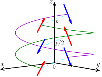
Figure 1: (Color online) A schematic illustration of a single period of a typical spin helix state. Here, $p=2\pi/\kappa$ denotes the pitch of the helix whose wave vector is $\kappa$. The solid curves depict the helical trajectories of two points on the $z=0$ plane, and the arrows point along the local direction of magnetization. If the state hosts vortices, their cores will also follow similar trajectories.

III Results

We have solved the reduced GP equation, Eq. (3), for various values of the helical wave vector $\kappa$ and the dipolar coupling constant $g_{\mathrm{d}}$. In the numerical simulations, we choose the harmonic oscillator length $a_{r}=\sqrt{\hbar/m\omega_{r}}$ for the unit of length and $\hbar\omega_{r}$ for the unit of energy. For definiteness, we fix the value of the dimensionless density–density coupling constant to $\tilde{g}=gN/\hbar\omega_{r}a_{r}^{2}=10^{3}$, which corresponds roughly to $1.5\times 10^{4}$ ${}^{87}{\rm Rb}$ ${\rm atoms}/\mu{\rm m}$ in a trap with $a_{r}=1\,\mu{\rm m}$.

One particular class of stationary solutions is illustrated in Fig. 2 with $g_{\mathrm{d}}=0.10\,g$. On the left-hand side, Figs. 2(a)–2(c), the state is shown in the axially homogeneous case, $\kappa=0$, and on the right-hand side, Figs. 2(d)–2(f), with finite helical pitch, $\kappa=0.25\,{\rm rad}/a_{r}$. The left column in each subfigure shows the amplitudes of the order-parameter components $|\psi_{1}|$, $|\psi_{0}|$, and $|\psi_{-1}|$, from up to down. The complex phases of the corresponding components are given in the right column in each subfigure. For both states, the magnetization is pointing predominantly in the positive $z$ direction in the upper half $(y>0)$ and in the negative $z$ direction in the lower half $(y<0)$ of the $xy$ plane.

The complex-phase plots in Figs. 2(a)–2(c) reveal that the system is hosting two integer-spin vortices with phase windings $(0,1,2)$ (upper half) and $(-2,-1,0)$ (lower half) in the components ($\psi_{1}$, $\psi_{0}$, $\psi_{-1}$), respectively. The ferromagnetic cores of the vortices are deformed into elliptic shapes, which is also indicated by the separation of the phase singularities in the $\psi_{\pm 1}$ components, cf. Ref. Simula2010 . The two vortices carry both spin- and mass currents: the spin currents flow in the same direction whereas the mass currents flow in the opposite directions, canceling the total mass current in the state.

For finite helical wave vector, $\kappa>0$, the vortices move closer to the surface of the cloud, as illustrated in Figs. 2(d)–2(f). Not only do the cores of the vortex pair separate farther apart for larger $\kappa$, but also the separation between the singularities in the $\psi_{\pm 1}$ components increases. However, one should note that for larger $\kappa$, the vortex lines are tilted steeper with respect to the axial direction. Due to the structure of the topological defects hosted by the order parameter, we refer to this state as the Mermin–Ho vortex (MHV) helix. This type of solution is found to exist in the whole stability range of the system, $0\leq g_{\mathrm{d}}/g\lesssim 0.24$.

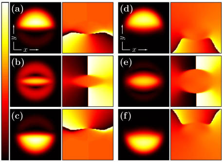
Figure 2: (Color online) Illustration of the MHV helix state for $g_{\mathrm{d}}=0.10\,g$ with $\kappa=0$ in (a)–(c) and $\kappa=0.25\,{\rm rad}/a_{r}$ in (d)–(f). For both states, the amplitudes of the order-parameter components ($\psi_{1}$, $\psi_{0}$, $\psi_{-1}$) are given in the left column and the complex phases in the right column. This class of states hosts a pair of MHVs with aligned spin currents and opposite mass flows. For each state separately, the color-map range in the left column is $\big{[}0,{\rm max}\left\{n({\bf r})\right\}\big{]}$ and in right column $\big{[}0,2\pi\big{]}$. The field of view in each panel is $[14\,a_{r}\times 14\,a_{r}]$.

The MHV helix is the ground-state texture within the symmetry requirements of Eqs. (6) for all parameter values considered in this work. However, there exists an interesting class of excited states which is illustrated in Fig. 3 for $g_{\mathrm{d}}=0.10\,g$ with $\kappa=0$ and $\kappa=1.0\,{\rm rad}/a_{r}$ on the left- and right-hand side, respectively. The complex-phase plots of Figs. 3(a) and 3(c) reveal that the state hosts two spin vortices with the same phase windings $(-1,0,1)$ in the components $(\psi_{1},\psi_{0},\psi_{-1})$, respectively. These defects are spin vortices with polar (nonmagnetized) core regions. Such vortices carry a spin current, whereas the mass current about the vortex line vanishes. The polar vortex cores within the ferromagnetic cloud are energetically analogous to air bubbles in water, hence increasing the total energy of the system through spin–spin interactions. The third singularity visible in Figs. 3(a) and 3(c) shows that the state hosts also a pair of fractional half-quantum vortices close to the surface of the cloud. However, these defects have very little effect on the texture because the related phase gradients lie in regions of nearly vanishing component amplitude $|\psi_{\pm 1}|$ for all values of $\kappa$.

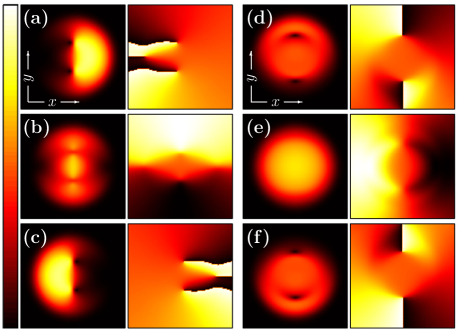
Figure 3: (Color online) Illustration of the PCV helix state for $g_{\mathrm{d}}=0.10\,g$ with $\kappa=0$ in (a)–(c) and $\kappa=1.0\,{\rm rad}/a_{r}$ in (d)–(f). For both states, the amplitudes of the order-parameter components ($\psi_{1}$, $\psi_{0}$, $\psi_{-1}$) are given in the left column and the complex phases in the right column. This class of states hosts a pair of PCVs with aligned spin currents and vanishing mass flows. For each state separately, the color-map range in the left column is $\big{[}0,{\rm max}\left\{n({\bf r})\right\}\big{]}$ and in right column $\big{[}0,2\pi\big{]}$. The field of view in each panel is $[14\,a_{r}\times 14\,a_{r}]$.

Solutions with similar vortex structures also exist for finite helical wave vectors, as depicted in Figs. 3(d)–3(f) for $\kappa=1.0\,{\rm rad}/a_{r}$. Thus, we refer to this state as the polar-core vortex (PCV) helix. This class of stationary states is found within the dipolar stability range of the system, except for weak dipolar interaction strengths, $g_{\mathrm{d}}/g\lesssim 10^{-3}$, likely due to numerical difficulties.

If one considers the vortex pairs in Figs. 2 and 3 as single entities, the total phase windings in both states are $(-2,0,2)$ in the order-parameter components $(\psi_{1},\psi_{0},\psi_{-1})$, respectively. By tracing the order parameter about the $z$-axis along a path close to the surface of the condensate, the expectation value of the spin rotates a total angle of $4\pi$ about the axial direction. This suggests that both states represent doubly quantized spin vortices that have split into different kinds of singly quantized spin defects. The splitting of doubly quantized mass vortices in scalar condensates has been studied previously both experimentally and numerically Shin2004 ; Mottonen2003 ; Huhtamaki2006 ; Mateo2006 .

The spin textures of the states depicted in Figs. 2 and 3 are shown in Fig. 4. Figures 4(a) and 4(b) illustrate the planar magnetization ${\bf M}^{\prime}(r,\varphi)$ for the MHV helix and Figs. 4(c) and 4(d) for the PCV helix. The projection of magnetization on the $xy$ plane, ${\bf M}^{\prime}_{xy}(r,\varphi)=M^{\prime}_{x}(r,\varphi){\bf e}_{x}+M^{\prime}_{y}(r,\varphi){\bf e}_{y}$, is depicted by the cones, with the length of each cone being proportional to the local magnitude $\sqrt{M^{\prime 2}_{x}(r,\varphi)+M^{\prime 2}_{y}(r,\varphi)}$. The axial magnetization, $M^{\prime}_{z}(r,\varphi)$, is shown by color. At the center of the system in the axially homogeneous textures ($\kappa=0$) in Figs. 4(a) and 4(c), the magnetization is pointing perpendicular to $\nabla M^{\prime}_{z}(r,\varphi)$ in the MHV and parallel to $\nabla M^{\prime}_{z}(r,\varphi)$ in the PCV state. For the MHV helix, this relative orientation is maintained for all values of the helical wave vector $\kappa$. However, for the PCV helix, the relative orientation twists continuously with increasing $\kappa$ and finally locks into the symmetric configuration shown in Fig. 4(d) for $\kappa\sim 1\,{\rm rad}/a_{r}$.

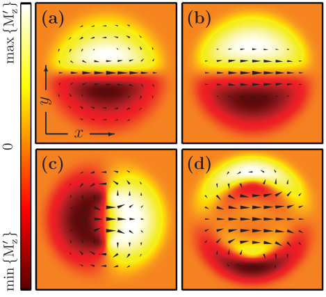
Figure 4: (Color online) Illustration of the spin textures for the states shown in Figs. 2 and 3. Panels (a) and (b) correspond to the MHV helix state with $\kappa=0$ and $\kappa=0.25\,{\rm rad}/a_{r}$, respectively. Panels (c) and (d) refer to the PCV helix state with $\kappa=0$ and $\kappa=1.0\,{\rm rad}/a_{r}$, respectively. The cones show the projection of magnetization onto the $xy$ plane and the color indicates the local value of axial magnetization $M^{\prime}_{z}(x,y)$. The field of view in each panel is $[13\,a_{r}\times 13\,a_{r}]$.

In Fig. 5, the total energy per particle, $E_{\rm tot}$, is shown as a function of the helical wave vector $\kappa$ for the MHV and the PCV helices. As previously, the coupling constants have the values $\tilde{g}=1000$ and $g_{\mathrm{d}}/g=0.10$ for both states. The MHV helix is the ground-state texture, within the constraints of Eq. (6), for all values of $\kappa$. Whereas $E_{\rm tot}$ for PCV helix is minimized for the axially homogeneous state, $\kappa=0$, the MHV helix is stabilized for a finite wave vector $\kappa_{\rm min}$. This minimum persists in the total energy for all positive interaction strengths $g$ and $g_{\mathrm{d}}$ considered. However, the relative magnitude of the dip, $\left[E_{\rm tot}(0)-E_{\rm tot}(\kappa_{\rm min})\right]/E_{\rm tot}(0)$, decreases for weaker dipolar interaction strengths. The curve $E_{\rm tot}(\kappa)$ is roughly a shifted parabola, closely resembling the result that long-period helical structures in MnSi and FeGe can become stable due to ferromagnetic Dzyaloshinskii instability Bak1980 .

The energy-minimizing helical wave vector $\kappa_{\rm min}$ is shown in Fig. 5(b) as a function of the dipolar interaction strength $g_{\mathrm{d}}/g$ for two values of the dimensionless coupling constant, $\tilde{g}=1000$ (solid curve) and $\tilde{g}=200$ (dashed curve). In the absence of dipolar interactions, the total energy is minimized by the axially homogeneous texture for which the kinetic energy is minimal. The value of $\kappa_{\rm min}$ increases rapidly as a function of $g_{\mathrm{d}}/g$ because the dipolar interactions, which overwhelm the kinetic energy already for $g_{\mathrm{d}}/g\approx 0.01$, favor a finite helical pitch. In general, $\kappa_{\rm min}$ increases for stronger dipolar couplings. However, the pitch of the energy-minimizing helix, $p_{\rm min}=2\pi/\kappa_{\rm min}$, is not determined directly by the dipole–dipole coherence length $\xi_{\rm dd}=\hbar/\sqrt{2mg_{\mathrm{d}}n(0)}$, where $n(0)$ is the particle density at the trap center. In fact, the coherence length $\xi_{\rm dd}$ shrinks for larger particle numbers, whereas $p_{\rm min}$ typically increases. This is likely due to the overall expansion of the condensate.

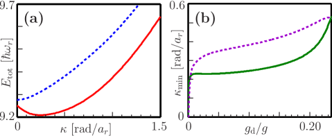
Figure 5: (Color online) (a) Total energy per particle, $E_{\rm tot}$, as a function of the helical wave vector $\kappa$ for the MHV helix (solid curve) and the PCV helix (dashed curve) with $\tilde{g}=1000$ and $g_{\mathrm{d}}/g=0.10$. The total energy of the MHV helix exhibits a local minimum with a finite wave vector $\kappa_{\rm min}$. (b) The energy-minimizing wave vector $\kappa_{\rm min}$ for the MHV helix as a function of the dipolar interaction strength $g_{\mathrm{d}}/g$ for two values of the density–density coupling constant, $\tilde{g}=1000$ (solid curve) and $\tilde{g}=200$ (dashed curve).

As a measure of how large the axial magnetization $M_{z}({\bf r})$ is on average, we define the integrated axial magnetization per unit length as $\mathcal{M}_{z}=\int d^{2}r|M^{\prime}_{z}(r,\varphi)|$. Similarly, the integrated transversal magnetization is given by $\mathcal{M}_{r}=\int d^{2}r\sqrt{M^{\prime 2}_{x}(r,\varphi)+M^{\prime 2}_{y}(r,\varphi)}$. These quantities are plotted in Figs. 6(a)–6(d) as functions of the helical wave vector $\kappa$ for $\tilde{g}=1000$ and four different values of the dipolar coupling constant $g_{\mathrm{d}}/g$. The solid curve corresponds to $\mathcal{M}_{r}$ and the dashed curve to $\mathcal{M}_{z}$. As shown in Fig. 6(a), the axial magnetization vanishes when $g_{\mathrm{d}}/g=0$. For $\kappa\gtrsim 0.7\,{\rm rad}/a_{r}$, the system becomes nonmagnetized because the additional kinetic energy due to finite $\kappa$ for magnetized states exceeds the energy gain from the spin–spin interaction, cf. Ref. Cherng2008 . Already for weak dipolar coupling, $g_{\mathrm{d}}/g=10^{-3}$, which is roughly the value for ${}^{87}{\rm Rb}$, the axial magnetization becomes significant, as shown in Fig. 6(b). Also, for finite dipolar coupling, the value of $\kappa$ at which the system enters a polar state is increased. The axial component of magnetization becomes larger for increasing $g_{\mathrm{d}}$, as illustrated in Figs. 6(c) and 6(d).

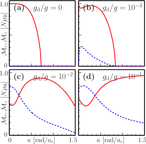
Figure 6: (Color online) Integrated transversal $\mathcal{M}_{r}$ (solid curve) and axial $\mathcal{M}_{z}$ (dashed curve) magnetization per unit length as a function of the helical wave vector $\kappa$ for the MHV helix. The strength of the dipolar coupling $g_{\mathrm{d}}/g$ is indicated in each panel. The overall magnetization is reduced for larger values of $\kappa$, and the axial magnetization tends to increase with $g_{\mathrm{d}}/g$.

IV Discussion

In summary, we have studied helical spin textures in a spin-1 BEC subject to long-range dipolar interactions. The axially elongated system was assumed to be confined radially by a cylindrically symmetric harmonic potential. By using a helical Ansatz, we reduced the zero-temperature GP equation to a two-dimensional problem, in which the helical wave vector $\kappa$ appeared as a parameter. This allowed us to investigate states with variable values of $\kappa$. We found two classes of helical solutions which we refer to as the Mermin–Ho and the polar-core vortex helices, according to the structure of their topological defects. Whereas the total energy of the polar-core vortex helix is minimized for the axially homogeneous case, $\kappa=0$, the Mermin–Ho vortex helix is stabilized for a finite pitch.

The helical spin textures studied in this work are naturally most transparent in elongated systems, such as cigar-shaped BECs. One difficulty in observing them as stable configurations in a condensate subject to weak dipolar interactions is that the spins tend to align predominantly parallel to the weak axis of the trap due to the head-to-tail attraction of the dipoles Yi2006 ; Takahashi2007 ; Huhtamaki2010 . However, we have performed additional three-dimensional simulations indicating that this problem can be overcome by placing the cigar-shaped system in a one-dimensional optical lattice potential. A strong enough lattice deforms the elongated condensate into a series of oblate clouds. Within each cloud, the preferred direction of magnetization lies perpendicular to the weak axis of the trap, and the relative orientation of magnetization between neighboring systems is determined by the long-range part of the interaction potential, i.e., by dipolar forces.

In the three-dimensional simulations, we calculated the total energy of an axially spin-polarized state and a helical spin texture subject to the symmetry constraint in Eq. (6) as a function of the strength of the optical lattice potential. We chose the aspect ratio of the confining harmonic potential such that $\omega_{z}/\omega_{r}=0.10$, where $\omega_{z}$ and $\omega_{r}$ are the axial and radial trapping frequencies, respectively. The values of the dimensionless coupling constants were fixed to $\tilde{g}=5\times 10^{4}$, $g_{\mathrm{s}}/g=-10^{-2}$, and $g_{\mathrm{d}}/g=10^{-3}$, corresponding to $8\times 10^{5}$ ${}^{87}{\rm Rb}$ atoms in a trap with $\omega_{r}=2\pi\times 100\,{\rm Hz}$. The optical lattice potential was of the form $V_{\rm opt}=E_{\mathrm{s}}\sin^{2}\left(k_{\mathrm{s}}z\right)$, where the constant $E_{\mathrm{s}}$ is the strength of the lattice potential, and the wave vector $k_{\mathrm{s}}$ determining the distance between neighboring clouds was fixed to $k_{\mathrm{s}}=\pi/10\,a_{r}$. The energy difference between the helical and polarized states was found to decrease monotonously as a function of $E_{\mathrm{s}}$, reaching degeneracy at $E_{\mathrm{s}}\approx 17\,\hbar\omega_{r}$.

Appendix A

Here, we calculate the dipolar integrals

$$I_{\beta}(r,\varphi,\kappa)=\sum_{\alpha}\int d^{3}r^{\prime}D_{\alpha\beta}({\bf r}-{\bf r}^{\prime})\big{|}_{z=0}M_{\alpha}({\bf r}^{\prime})$$ (7)

appearing in the reduced GP equation, Eq. (3). As shown below, the dipolar potential for a given magnetization can be efficiently evaluated by carrying out a series of one-dimensional Hankel transformations.

The expectation values of the spin operators $\hat{S}_{\alpha}$ are readily evaluated for the Ansatz in Eq. (2) by applying the Hadamard lemma. Recalling that quantities evaluated in the $z=0$ plane are denoted by primes, we obtain

$$M_{x}({\bf r}) = \cos(\kappa z)M^{\prime}_{x}(r,\varphi+\kappa z)+\sin(\kappa z)M^{\prime}_{y}(r,\varphi+\kappa z),$$

$$M_{y}({\bf r}) = -\sin(\kappa z)M^{\prime}_{x}(r,\varphi+\kappa z)+\cos(\kappa z)M^{\prime}_{y}(r,\varphi+\kappa z),$$

$$M_{z}({\bf r}) = M^{\prime}_{z}(r,\varphi+\kappa z).$$ (8)

The components of the planar magnetization are then expanded in polar Fourier series as

$$M^{\prime}_{\gamma}(r,\varphi)=\sum_{n}g_{\gamma}^{n}(r)e^{in\varphi},$$ (9)

where $g_{\gamma}^{n}(r)=\int d\varphi M^{\prime}_{\gamma}(r,\varphi)e^{-in\varphi}/2\pi=\left[g_{\gamma}^{-n}(r)\right]^{*}$. For the helical textures, the components $M^{\prime}_{\gamma}$ are in general slowly varying functions of the azimuthal angle $\varphi$, and hence they are accurately approximated by only a few terms in the expansion. The components of magnetization can be written in the form

$$M_{\alpha}({\bf r})=\sum_{s,n,\gamma}C_{\alpha\gamma}^{s}g_{\gamma}^{n}(r)e^{i\left[s\kappa z+n(\varphi+\kappa z)\right]},$$ (10)

where $s\in\{1,0,-1\}$ and the coefficients arising from the trigonometric functions in Eqs. (A) are given by $C^{s}_{xx}=C^{s}_{yy}=s^{2}/2$, $C^{0}_{zz}=1$, $C^{s}_{xy}=-C^{s}_{yx}=is/2$, and $0$ otherwise.

Each of the three terms in Eq. (7) is a convolution. By applying the convolution theorem, we obtain

$$I_{\beta}(r,\varphi,\kappa)=\sum_{\alpha}\hat{\mathcal{F}}^{-1}\left\{K_{\alpha\beta}({\bf k})\hat{\mathcal{F}}M_{\alpha}({\bf r})\right\}_{z=0},$$ (11)

where $\hat{\mathcal{F}}$ stands for the Fourier transform. The functions $K_{\alpha\beta}({\bf k})=\hat{\mathcal{F}}D_{\alpha\beta}({\bf r})$ can be written in cylindrical coordinates $(k,\theta,k_{z})$ as

$$K_{\alpha\beta}(k,\theta,k_{z})=\pi\sum_{\ell=-2}^{2}K_{\alpha\beta}^{\ell}(k_{z}/k)e^{i\ell\theta},$$ (12)

where $K^{\pm 2}_{xx}=-K^{\pm 2}_{yy}=\pm iK^{\pm 2}_{xy}=L(\xi)\equiv 1/(1+\xi^{2})$, $K^{\pm 1}_{xz}=\pm iK^{\pm 1}_{yz}=2\xi L(\xi)$, $K^{0}_{xx}=K^{0}_{yy}=-4/3+2L(\xi)$, $K^{0}_{zz}=-4/3+4\xi^{2}L(\xi)$, $K^{\ell}_{\alpha\beta}=K^{\ell}_{\beta\alpha}$, and $0$ otherwise.

The Fourier transforms of the components of magnetization in Eq. (11) are readily evaluated with the aid of the Jacobi–Anger expansion, and the result is

$$\hat{\mathcal{F}}M_{\alpha}({\bf r})=(2\pi)^{2}\sum_{\gamma,s,n}C_{\alpha\gamma}^{s}(-i)^{n}H^{n}_{\gamma}(k)e^{in\theta}\delta(\kappa(s+n)-k_{z}),$$ (13)

where $H_{\gamma}^{n}(k)=\int rdrJ_{n}(kr)g_{\gamma}^{n}(r)$ is the $n$th order Hankel transformation of $g_{\gamma}^{n}$. By substituting Eqs. (12) and (13) into Eq. (11) and carrying out the integration over $k_{z}$, we obtain

$$I_{\beta}(r,\varphi,\kappa) = 2\pi^{2}\sum_{\stackrel{{\scriptstyle\alpha,\gamma,s}}{{n,\ell}}}C_{\alpha\gamma}^{s}(-i)^{n}$$

$$\times\hat{\mathcal{F}}^{-1}_{2D}\left\{K_{\alpha\beta}^{\ell}(q)H_{\gamma}^{n}(k)e^{i(n+\ell)\theta}\right\},$$

where $q=\kappa(s+n)/k$ and $\hat{\mathcal{F}}^{-1}_{2D}$ denotes the inverse Fourier transform in the $z=0$ plane. Again, the inverse Fourier transforms can be evaluated by applying the Jacobi–Anger expansion, resulting in

$$I_{\beta}(r,\varphi,\kappa)=\pi\sum_{n,\ell}i^{\ell}h^{n\ell}_{\beta}(r)e^{i(n+\ell)\varphi},$$ (15)

where $h^{n\ell}_{\beta}(r)=\int kdkJ_{n+\ell}(kr)f_{\beta}^{n\ell}(k,\kappa)$ stands for the inverse Hankel transformation of order $n+\ell$ of the function $f_{\beta}^{n\ell}(k,\kappa)=\sum_{\alpha,\gamma,s}C_{\alpha\gamma}^{s}K_{\alpha\beta}^{\ell}(q)H_{\gamma}^{n}(k)$. By denoting $q_{\pm}=\kappa(n\pm 1)/k$ and $q_{0}=\kappa n/k$, these functions can be written as

$$f_{x}^{n,\pm 2} = \left(H_{x}^{n}\mp iH_{y}^{n}\right)L(q_{\pm})=\pm if_{y}^{n,\pm 2},$$ (16)

$$f_{x}^{n,\pm 1} = 2H_{z}^{n}q_{0}L(q_{0})=\pm if_{y}^{n,\pm 1},$$ (17)

$$f_{x}^{n,0} = 2\left(H_{x}^{n}\mp iH_{y}^{n}\right)\left[-\frac{2}{3}+L(q_{\pm})\right]\pm if_{y}^{n,0},$$ (18)

$$f_{z}^{n,\pm 1} = 2\left(H_{x}^{n}\mp iH_{y}^{n}\right)q_{\pm}L(q_{\pm}),$$ (19)

$$f_{z}^{n,0} = 2H_{z}^{n}\left[-\frac{2}{3}+2q_{0}^{2}L(q_{0})\right],$$ (20)

where $f_{x}^{n,0}$ and $f_{y}^{n,0}$ are given implicitly through Eq. (18).

In the case of an axially polarized cylindrically symmetric state, $\psi_{k}=\sqrt{n(r)}\delta_{1k}$, the GP equation, Eq. (II), is reduced to a scalar equation. In this simple case, $g^{0}_{z}$ yields the only non-vanishing term in Eq. (9), which, together with the fact that $q_{0}=0$, implies that $f^{0,0}_{z}=-4H^{0}_{z}/3$ is the only non-vanishing function in Eqs. (16)–(20). Substitution into Eq. (15) shows that Eq. (II) is reduced into the scalar equation if we replace $g\longrightarrow g+g_{\mathrm{s}}-\frac{4\pi}{3}g_{\mathrm{d}}$, which is readily proved also by direct evaluation of Eq. (11).

References

- (1) J. D. Watson and F. H. C. Crick, Nature 171, 737 (1953).
- (2) M. Vengalattore, S. R. Leslie, J. Guzman, and D. M. Stamper-Kurn, Phys. Rev. Lett. 100, 170403 (2008).
- (3) R. W. Cherng, V. Gritsev, D. M. Stamper-Kurn, and E. Demler, Phys. Rev. Lett. 100, 180404 (2008).
- (4) S. Yi and H. Pu, Phys. Rev. Lett. 97, 020401 (2006).
- (5) Y. Kawaguchi, H. Saito, and M. Ueda, Phys. Rev. Lett. 97, 130404 (2006).
- (6) M. Takahashi, S. Ghosh, T. Mizushima, and K. Machida, Phys. Rev. Lett. 98, 260403 (2007).
- (7) J. A. M. Huhtamäki, M. Takahashi, T. P. Simula, T. Mizushima, and K. Machida, Phys. Rev. A 81, 063623 (2010).
- (8) Y. Kawaguchi, H. Saito, and M. Ueda, Phys. Rev. Lett. 98, 110406 (2007).
- (9) V. Bretin, P. Rosenbusch, F. Chevy, G. V. Shlyapnikov, and J. Dalibard, Phys. Rev. Lett. 90, 100403 (2003).
- (10) T. Mizushima, M. Ichioka, and K. Machida, Phys. Rev. Lett. 90, 180401 (2003).
- (11) A. L. Fetter, Phys. Rev. A 69, 043617 (2004).
- (12) T. P. Simula, T. Mizushima, and K. Machida, Phys. Rev. Lett. 101, 020402 (2008).
- (13) Y. M. Cho, H. Khim, and P. Zhang, Phys. Rev. A 72, 063603 (2005).
- (14) A. Griesmaier, J. Werner, S. Hensler, J. Stuhler, and T. Pfau, Phys. Rev. Lett. 94, 160401 (2005).
- (15) Q. Beaufils, R. Chicireanu, T. Zanon, B. Laburthe-Tolra, E. Maréchal, L. Vernac, J.-C. Keller, and O. Gorceix, Phys. Rev. A 77, 061601(R) (2008).
- (16) D. Sukachev, A. Sokolov, K. Chebakov, A. Akimov, S. Kanorsky, N. Kolachevsky, and V. Sorokin, Phys. Rev. A 82, 011405(R) (2010).
- (17) A. J. Berglund, J. L. Hanssen, and J. J. McClelland, Phys. Rev. Lett. 100, 113002 (2008).
- (18) M. Lu, S. H. Youn, and B. L. Lev, Phys. Rev. Lett. 104, 063001 (2010).
- (19) N. N. Klausen, J. L. Bohn, and C. H. Greene, Phys. Rev. A 64, 053602 (2001).
- (20) E. G. M. van Kempen, S. J. J. M. F. Kokkelmans, D. J. Heinzen, and B. J. Verhaar, Phys. Rev. Lett. 88, 093201 (2002).
- (21) A. Widera, F. Gerbier, S. Fölling, T. Gericke, O. Mandel, and I. Bloch, New J. Phys. 8, 152 (2006).
- (22) T. P. Simula, J. A. M. Huhtamäki, M. Takahashi, T. Mizushima, and K. Machida, arXiv:1007.3551 .
- (23) T. Lahaye, C. Menotti, L. Santos, M. Lewenstein, and T. Pfau, Rep. Prog. Phys. 72, 126401 (2009).
- (24) P. O. Fedichev, Y. Kagan, G. V. Shlyapnikov, and J. T. M. Walraven, Phys. Rev. Lett. 77, 2913 (1996).
- (25) M. Theis, G. Thalhammer, K. Winkler, M. Hellwig, G. Ruff, R. Grimm, and J. Hecker Denschlag, Phys. Rev. Lett. 93, 123001 (2004).
- (26) Y. Shin, M. Saba, M. Vengalattore, T. A. Pasquini, C. Sanner, A. E. Leanhardt, M. Prentiss, D. E. Pritchard, and W. Ketterle, Phys. Rev. Lett. 93, 160406 (2004).
- (27) M. Möttönen, T. Mizushima, T. Isoshima, M. M. Salomaa, and K. Machida, Phys. Rev. A 68, 023611 (2003).
- (28) J. A. M. Huhtamäki, M. Möttönen, T. Isoshima, V. Pietilä, and S. M. M. Virtanen, Phys. Rev. Lett. 97, 110406 (2006).
- (29) A. M. Mateo and V. Delgado, Phys. Rev. Lett. 97, 180409 (2006).
- (30) P. Bak and M. H. Jensen, J. Phys. C: Solid State Phys. 13, L881 (1980).