Convergence of Income Growth Rates in
Evolutionary Agent-Based Economics

Abstract.

We consider a heterogeneous agent-based economic model where economic agents have strictly bounded rationality and where income allocation strategies evolve through selective imitation. Income is calculated by a Cobb-Douglas type production function, and selection of strategies for imitation depends on the income growth rate they generate. We show that under these conditions, when an agent adopts a new strategy, the effect on its income growth rate is immediately visible to other agents, which allows a group of imitating agents to quickly adapt their strategies when needed.

Departament de Ciències Matemàtiques i Informàtica
Universitat de les Illes Balears

1. Introduction

In biology, fitness describes the capability of an individual of a certain genotype to reproduce. In analogy, fitness in this context of evolutionary economics describes the likelihood that an agent with a certain behavior is imitated by other agents. If the likelihood that an agent with a certain investment strategy is imitated depends on the relative income growth rate of the agent, the functional relationship between investment strategies and income growth rates is central to the understanding of the emerging evolutionary dynamics, and can be used to develop new economic policy tools (see for example Nannen and van den Bergh, 2010). Here we study how the income growth rate of an agent stabilizes after a change of strategy, i.e., how it converges to the equilibrium growth rate that an imitating agent realizes if it holds on to a particular investment strategy and when prices are stable. In particular, we want to know if there is significant delay between the adoption of a new strategy and the expression of this strategy in terms of income growth.

2. Strategies, growth and production

In this model, agents represent firms. Each agent formulates an investment strategy that specifies how current income is invested in a finite number of capital sectors, e.g., security, machinery, or sales infrastructure. The returns for each agent are then calculated from standard economic growth and production functions. We do not model savings, and so the income growth rate is also the growth rate of returns on investments. Some allocations give higher returns than others, and the goal of the agents is to find a strategy that can realize a high level of individual welfare. Agents have bounded rationality and limited information. They observe the investment strategy and resulting income growth rate of other agents, and imitate a successful investment strategy, possibly with some variation. This constitutes a collective learning process, where strategies evolve by selection and variation.

Let $n$ be the number of available investment sectors. Formally, the investment strategy ${s}_{a}({t})$ of agent ${a}$ at time ${t}$ can be defined as an $n$-dimensional vector

(1) $${s}_{a}({t})=\left[0,1\right]^{n},\quad\sum_{i}{s}_{i{a}}({t})=1.$$

Let ${Y}_{a}({t})$ be the income of agent ${a}$ at time ${t}$. The partial strategy ${s}_{i{a}}({t})$—which is the $i^{th}$ element of a strategy—determines the fraction ${s}_{i{a}}({t}){Y}_{a}({t}-1)$ of income that agent ${a}$ invests in sector $i$ at time ${t}$. As agents allocate all of their income over the available sectors, the partial strategies must be non-negative and sum to one. The set of all possible investment strategies forms an $n-1$ dimensional simplex that is embedded in $n$-dimensional Euclidean space.

We use standard economic growth and production functions to describe how capital accumulates in each sector and contributes to income. These functions are not aggregated: growth and returns are calculated independently for each agent. We consider invested capital to be non-malleable: once invested it cannot be transferred between sectors. Capital accumulation in each sector depends on the sector specific investment of each agent, a dynamic price $p_{i}({t})$, and the global deprecation rate ${\delta}$. Deprecation is assumed to be equal for all sectors and all agents. The difference equation for non-aggregate growth per sector is

(2) $${K}_{i{a}}({t})=\frac{{s}_{i{a}}({t})}{p_{i}({t})}{Y}_{a}({t}-1)+(1-{\delta}){K}_{i{a}}({t}-1).$$

To calculate the income ${Y}_{a}({t})$ from the capital that agent ${a}$ has accumulated per sector, we use an $n$-factor Cobb-Douglas production function with constant elasticity of substitution,

(3) $${Y}_{a}({t})={\beta}\prod_{i}{{K}_{i{a}}({t})}^{{\alpha}_{i}},$$

where ${\beta}$ is a scaling factor that limits the maximum possible income growth rate. The relative contribution of each sector to production is expressed by a vector of non-negative production coefficients ${\alpha}=\langle{\alpha}_{1}\ldots{\alpha}_{n}\rangle$. To enforce constant returns to scale, all production coefficients are constraint to add up to one,

(4) $${\alpha}=\left[0,1\right]^{n},\quad\sum_{i}{\alpha}_{i}({t})=1.$$

Similar to the strategy space, the set of all possible vectors of production coefficients is an $n-1$ dimensional simplex that is embedded in $n$-dimensional Euclidean space.

3. The equilibrium growth rate

To find the equilibrium growth rate, we start with an analysis of the equilibrium ratio of sector specific capital to income that will be achieved if an agent holds on to a particular strategy. The difference equation of this ratio is

(5) $$\frac{{K}_{i{a}}({t})}{{Y}_{a}({t})}= \frac{\nicefrac{{{s}_{i{a}}({t})}}{{p_{i}({t})}}{Y}_{a}({t}-1)\;+\;(1-{\delta}){K}_{i{a}}({t}-1)}{({\gamma}_{a}({t})+1)\;{Y}_{a}({t}-1)}$$

$$= \frac{{s}_{i{a}}({t})/p_{i}({t})}{{\gamma}_{a}({t})+1}+\frac{1-{\delta}}{{\gamma}_{a}({t})+1}\;\frac{{K}_{i{a}}({t}-1)}{{Y}_{a}({t}-1)}.$$

This dynamic equation is of the form

$$x({t})=a+bx({t}-1),$$

which under the condition $0\!\leq\!b\!<\!1$ converges monotonously to its unique stable equilibrium at

$$\lim_{{t}\to\infty}x({t})\!=\!a/(1-b).$$

This condition is fulfilled here: investment is always non-negative and sector specific capital cannot decrease faster than ${\delta}$. With constant returns to scale, income cannot decline faster than capital deprecation, i.e., ${\gamma}_{a}\!\geq\!-{\delta}$. For the moment, let us exclude the special case ${\gamma}_{a}\!=\!-{\delta}$. Then, considering that $0\!<\!{\delta}\!\leq\!1$, we have the required constraint

(6) $$0\leq\frac{1-{\delta}}{{\gamma}_{a}({t})+1}<1.$$

We conclude that the ratio of capital to income converges to

(7) $$\lim_{{t}\to\infty}\frac{{K}_{i{a}}({t})}{{Y}_{a}({t})}= \lim_{{t}\to\infty}\frac{{s}_{i{a}}({t})/p_{i}({t})}{{\gamma}_{a}({t})+1}/\left(1-\frac{1-{\delta}}{{\gamma}_{a}({t})+1}\right)$$

$$= \lim_{{t}\to\infty}\,\frac{{s}_{i{a}}({t})/p_{i}({t})}{{\gamma}_{a}({t})+{\delta}}.$$

The existence of this limit depends on the behavior of $p_{i}({t})$. If prices converge, equation 7 describes a unique stable equilibrium to which the ratio of capital to income converges monotonously. We ignore the limit notation and combine equation 7 with equation 3 to calculate income at equilibrium as

(8) $${Y}_{a}({t}) ={\beta}\,\prod_{i}\left(\frac{{s}_{i{a}}({t})/p_{i}({t})}{{\gamma}_{a}({t})+{\delta}}{Y}_{a}({t})\right)^{{\alpha}_{i}}$$

$$=\frac{{\beta}\,{Y}_{a}({t})}{{\gamma}_{a}({t})+{\delta}}\,\prod_{i}p_{i}({t})^{-{\alpha}_{i}}\,\prod_{i}{s}_{i{a}}({t})^{{\alpha}_{i}}.$$

We can now solve for ${\gamma}_{a}({t})$ to derive the equilibrium growth rate

(9) $${\gamma}_{a}({t})={\beta}\,\prod_{i}p_{i}({t})^{-{\alpha}_{i}}\,\prod_{i}{s}_{i{a}}({t})^{{\alpha}_{i}}-{\delta}.$$

Let us return to the special case ${\gamma}_{a}=-{\delta}$. According to equation 2, capital per sector decreases at the deprecation rate ${\delta}$ only when it receives zero investment, and it cannot decrease faster. With constant elasticity of substitution, a growth of ${\gamma}_{a}=-{\delta}$ is only possible if every sector with a positive production coefficient receives zero investment. This implies ${s}_{i{a}}({t})=0$ for at least one partial strategy, and so equation 9 holds also for the special case ${\gamma}_{a}=-{\delta}$.

4. Relative order of strategies

The scaling factor ${\beta}$, the price $p$ and the deprecation rate ${\delta}$ are monotonous transformations of the equilibrium growth rate in equation 9. They do not affect the order of strategies with respect to the income growth rate at equilibrium. Whether one investment strategy results in a higher income growth rate at equilibrium than another investment strategy depends solely on the term $\prod_{i}{s}_{i{a}}({t})^{{\alpha}_{i}}$. Further to this, a set of investment strategies with identical equilibrium growth rate, say ${\gamma}^{\prime}$, forms a contour hyper surface in the strategy simplex. All strategies that are enveloped by this hyper surface have a higher equilibrium growth rate ${\gamma}_{a}({t})\geq{\gamma}^{\prime}$. This inner set is convex (for a related proof see Beer, 1980) and satisfies

(10) $$\prod_{i}{s}_{i{a}}({t})^{{\alpha}_{i}}\geq\frac{{\gamma}^{\prime}+{\delta}}{{\beta}}\prod_{i}p_{i}({t})^{{\alpha}_{i}}.$$

Maximizing this type of equilibrium growth rate poses no challenge to a (collective) learning mechanism. It has a single global maximum at ${s}_{a}({t})\!=\!{\alpha}$, no local maxima, and a distinct slope that increases away from the maximum, allowing even the simplest of hill climbing algorithms to find and approach it. Learning mechanisms will differ mostly in the speed of convergence and the degree of fine tuning at the optimum.

5. Convergence

Numerical simulations reveal that after an agent has changed its investment strategy, its income growth rate approaches the equilibrium growth rate of the new strategy always monotonously from above. This might be obvious when an agent exchanges a superior strategy for an inferior strategy. But it is also true when an agent exchanges an inferior for a superior strategy, because the change in the distribution of an agent’s total capital over the sectors is largest immediately after a change in the allocation of investments, with a strong effect on the income growth rate. Even when an agent switches between two strategies that have the same equilibrium growth rate, the agent will temporarily increase its income growth rate and approach the equilibrium growth rate from above. That is, the agent will sustain an equilibrium growth rate that is higher than (or equal to) the equilibrium growth rate of each of the two strategies on their own. This is due to the convex shape of the equilibrium growth rate. Any convex combination of two strategies with equal equilibrium growth rate must have an equilibrium growth rate at least as high as that of the two combining strategies. The temporal effect of a switch between two strategies is similar to that of a convex combination of the two strategies.

This peculiar convergence behavior introduces an intrinsic bias into the evolutionary process that favors an agent that has just changed its strategy. Figure 1 visualizes the behavior of the income growth rate of a single agent that changes its strategy several time over the course of 500 time steps. In this example the economy is calibrated such that the equilibrium growth rate of the optimal strategy is 1.85 percent per year. Each random strategy is another imitation (i.e., copy) of the optimum strategy with an imitation error that follows a Gaussian distribution ${\mathcal{N}}(0,0.02)$. Immediately after the imitation, the income growth rate of the imitating agent always exceeds the equilibrium growth of its new (and nearly optimal) strategy by a significant margin. Occasionally the actual growth exceeds even the equilibrium growth rate of the optimal strategy, which means that if at that moment another agent has to choose whether to imitate this agent or an agent that is using the optimal strategy, it is likely to imitate this agent.

Comparing the real income growth rate to the equilibrium growth rate

income growth rate

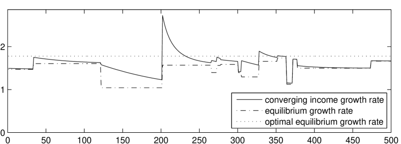
time steps

converging growth rate minus equilibrium growth rate

excess growth rate

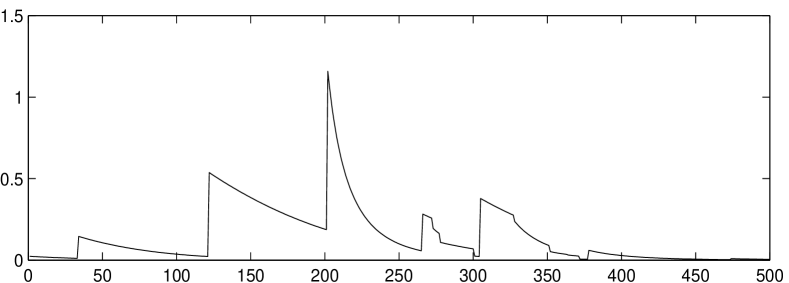
time steps

Figure 1. Income growth rate of a single agent during 500 time steps. The agent changes its strategy several times.

6. Conclusion

We conclude that if imitating agents base the decision from which agent to imitate on the income growth of their fellow agents, there is no delay between the adoption of a strategy (the genotype) and expression of this strategy in terms of economic performance (the phenotype), which is of great advantage to an evolutionary process that is based on imitation. However, the convergence behavior introduces significant biased in favor of those agents that have only recently changed their strategy. This might prevent an agent population to fully converge on the optimal strategy, and preserve variation in the pool of strategies.

References

- Beer (1980) Beer, G., 1980. The Cobb-Douglas Production Function. Mathematical Magazine 53 (1), 44–48.
- Nannen and van den Bergh (2010) Nannen, V., van den Bergh, J. C. J. M., 2010. Policy instruments for evolution of bounded rationality: Application to climate-energy problems. Technological Forecasting & Social Change 77, 76–93.