Tests of Non-Equivalence among Absolutely Nonsingular Tensors through Geometric Invariants

Sakata, T.¹, Maehra, K.², Sasaki,T.³, Sumi, T. ¹, Miyazaki, M.⁴ and Watanabe Y.⁵

Department of Design Human Science, Kyushu University¹
School of Design, Kyushu University².
Department of Mathematics, Kobe University³.
Department of Mathematics, Kyoto University of Education⁴
Research Institute of Information Technology, Kyushu University⁵

1 Introduction

Tensor data analysis has successfully developed in various application fields, which is useful to seize multi-factor dependence. An $n\times n\times p$ tensor is a multi-array datum $T=(T_{ijk}),$ where $1\leq i,j\leq n$ and $1\leq k\leq p.$ A type $n\times n\times p$ tensor $T$ is denoted by $T=(A_{1};A_{2};\cdots;A_{p})$ where $A_{i}$ denote $n\times n$ matrices. An $n\times n\times p$ tensor $T$ is said to be of rank $1$ if there is a vectors $\bm{a}=(a_{1},a_{2},...,a_{n}),$ $\bm{b}=(b_{1},b_{2},...,b_{n})$, and $\bm{c}=(c_{1},c_{2},...,c_{p})$ such that $T_{ijk}=a_{i}b_{j}c_{k}$ for all $i,j,k,$ and the rank of a tensor $T$ is defined as the minimum of the integer $r$ such that $T$ can be expressed as the sum of $r$ rank-one tensors. The maximal rank of all tensors of type $n\times n\times p$ are also defined in obvious fashion and denoted by ${\rm maxrank(n,n,p)}$.The rank of a tensor describes the complexity of a tensorial datum and the maximal rank describes the model complexity of a class of tensors of a given type, and so they are very important concepts in both applied and theoretical fields. Therefore, the rank and maximal rank determination problems have attracted the interest of many researchers, for example, Kruskal [12], ten-Berge [24], and Common et al, [6], etc. and now have being investigated intensively( for a comprehensive survey, see Kolda et al.[11]). Atkinson et al.([1] and [2] ) claimed that ${\rm maxrank}(n,n,3)\leq 2n-1$. Here we introduce an important class of tensors.

Definition 1.1

A real tensor $T=(A_{1};A_{2};,\dots;A_{p})$ is said to be absolutely nonsingular if $x_{1}A_{1}+x_{2}A_{2}+\cdots+x_{p}A_{p}$ is nonsingular for all $(x_{1},x_{2},...,x_{p})\neq(0,0,...,0).$

Remark 1.2

We called absolutely nonsingular tensors as exceptional tensors in Sakata et al. [21],[22].

Sumi et al.[23] proved the claim of Atkinson et al. over the complex number filed $\mathbb{C}$ without any assumption and proved it over the real number filed $\mathbb{R}$ except the class of absolutely nonsingular tensors. Thus, for the proof of the claim of Atkinson et al. over the real number filed $\mathbb{R},$ it is the first thing to determine all absolutely nonsingular tensors. Absolutely nonsingular tensors are characterized by the determinant polynomial defined below. Searching of absolutely nonsingular tensors was pursued in Sakata et al. [21],[22] in this direction. As well as searching absolutely nonsingular tensors, the equivalence among them under the rank-preserving transformation which is defined below is also important. Note that such equivalence relation has also a relation to the SLOCC equivalence of entangled states in the quantum communication (for example, see Chen et al. [5]).

Definition 1.3

For a $n\times n\times p$ tensor $T=(A_{1};A_{2};,\dots;A_{p}),$ the homogeneous polynomial in $x_{1},...,x_{p}$ of degree $n$

$$f_{T}(x_{1},x_{2},...,x_{p})=\det(x_{1}A_{1}+x_{2}A_{2}+\cdots+x_{p}A_{p})$$ (1.4)

is called the determinant polynomial of a tensor $T$.

Then we have the following important characterization.

Theorem 1.5

If $T=(A_{1};A_{2};,\dots;A_{p})$ is absolutely nonsingular, its determinant polynomial $f_{T}(x_{1},x_{2},...,x_{p})$ is a positive definite homogeneous polynomial or negative definite homogeneous polynomial.

Proof  Let $T=(A_{1};A_{2};,\dots;A_{p})$ be absolutely nonsingular, and assume that there are two points $\bm{x}_{0}$ and $\bm{x}_{1}$ such that $f_{T}(\bm{x}_{0})>0$ and $f_{T}(\bm{x}_{1})<0.$ The line $\ell$ combining the two points $\bm{x}_{0}$ and $\bm{x}_{1}$ must pass through the origin $\bm{0}$, since in the segment $[x_{0},x_{1}]$ there must be $\bm{x}^{\prime}$ such that $f_{T}(\bm{x}^{\prime})=0$ and it must be $\bm{0}$ because $T$ is absolutely nonsingular. Let take another point $\bm{x}_{2}$ which is not on the line $\ell$. Then, the line passing $\bm{x}_{0}$ and $\bm{x}_{2}$ does not pass the origin and so $f(\bm{x}_{0})f(\bm{x}_{2})<0$ is impossible just by the same reason given in the previous sentence. So, $f(\bm{x}_{0})f(\bm{x}_{2})>0.$ Next, consider the line passing $\bm{x}_{1}$ and $\bm{x}_{2}$, which also does not pass the origin and $f(\bm{x}_{1})f(\bm{x}_{2})<0$. This is also a contradiction. After all, there don’t exist points $\bm{x}_{0}$ and $\bm{x}_{1}$ such that $f(\bm{x}_{0})>0$ and $f(\bm{x}_{1})<0.$ This proves Theorem 1.5.  

It is well known that tensor rank is invariant by typical matrix transformations, say, $p-$, $q-$, and $r-$transformations defined below. So, equivalence relation of two tensors means that they have a same rank. Thus, to study equivalence among tensors is of some importance for rank determination.

Definition 1.6

For a $n\times n\times p$ tensor $T=(A_{1};A_{2};\cdots;A_{p}),$ the following transformations

• $T=(A_{1};A_{2};\cdots;A_{p})\rightarrow T^{\prime}=(PA_{1};PA_{2};\cdots;PA_{p})$ by an $n\times n$ matrix $P\in GL(n),$

• $T=(A_{1};A_{2};\cdots;A_{p})\rightarrow T^{\prime}=(A_{1}Q;PA_{2}Q;\cdots;A_{p}Q)$ by an $n\times n$ matrix $P\in GL(n),$

• $T=(A_{1};A_{2};\cdots;A_{p})\rightarrow T^{\prime}=(R_{11}A_{1}+R_{12}A_{2}+R_{13}A_{3};R_{21}A_{1}+R_{22}A_{2}+R_{23}A_{3};R_{31}A_{1}+R_{32}A_{2}+R_{33}A_{3})$ by a $p\times p$ matrix $P\in GL(n)$

are called as $p-$, $q-$, and $r-$transformations and denoted by $T\rightarrow_{p}T^{\prime},T\rightarrow_{q}T^{\prime}andT\rightarrow_{r}T^{\prime}$ respectively. Further, if $T_{1}\rightarrow_{p}T_{2}$, the $T_{1}$ and $T_{2}$ are said to be in the $p-$equivalence. $q-$ and $r-$equivalence are defined analogously.

Definition 1.7

Let $T_{1}=(A_{1};A_{2};\cdots;A_{p})$ and $T_{2}=(B_{1};B_{2};\cdots;B_{p})$ be two $n\times n\times p$ tensors. If there is a sequence of $\{T_{i}\}$ starting from $T_{1}$ and ending at $T_{2},$ in which $T_{i}$ and $T_{i+1}$ are in the relation of $p-$, or $q-$, or $r-$equivalence, then $T_{0}$ and $T_{1}$ are said to be equivalent.

Now we can reduce the equivalence relation into a more simple one by the following lemma.

Lemma 1.8

$p-$, $q-$ and $r-$transformations are mutually commutative.

Proof  For simplicity, we prove for $p=3$, however, the proof is similar for a general $p$. First we prove the commutativity of $p-$transformation and $r-$transformation. Let

$$T_{1}\rightarrow_{p}T_{2}\rightarrow_{r}T_{3}\ \ and\ \ T_{1}\rightarrow_{r}T^{{}^{\prime}}_{2}\rightarrow_{p}T^{{}^{\prime}}_{3}$$

We will show that $T_{3}=T^{{}^{\prime}}_{3}.$ Let $T_{1}=(A_{1};A_{2};A_{3})$ and $P=(p_{ij})$ and $R=(r_{ij}).$ Then,

$$T_{2}=(PA_{1};PA_{2};PA_{3})$$

and

$$T_{3}=(r_{11}PA_{1}+r_{12}PA_{2}+r_{13}PA_{3};r_{21}PA_{1}+r_{22}PA_{2}+r_{23}PA_{3};r_{31}PA_{1}+r_{32}PA_{2}+r_{33}PA_{3})$$

On the other hand

$$T^{{}^{\prime}}_{2}=(r_{11}A_{1}+r_{12}A_{2}+r_{13}A_{3};r_{21}A_{1}+r_{22}A_{2}+r_{23}A_{3};r_{31}A_{1}+r_{32}A_{2}+r_{33}A_{3})$$

and

$$T^{{}^{\prime}}_{3}=(r_{11}PA_{1}+r_{12}PA_{2}+r_{13}PA_{3};r_{21}PA_{1}+r_{22}PA_{2}+r_{23}PA_{3};r_{31}PA_{1}+r_{32}PA_{2}+r_{33}PA_{3})$$

Thus, $T_{3}=T^{{}^{\prime}}_{3},$ and this means the commutativity of $p$- and $r$-transformations. The commutativity of $q$- and $r$-transformations are proved similarly. $p$- and $q$-transformations are obviously commutative. This proves Lemma 1.8.  

Note that in this paper we consider three cases of (1) $P,Q\in GL(n)$ and $R\in GL(p)$ and (2) $P,Q\in GL(n)$ and $R\in SL(p).$ and (3) $P,Q\in SL(n)$ and $R\in SL(p).$ The first is called $GL(p)$-equivalence or simply equivalence, and the second is called $SL(p)$-equivalence in short. The third case is called, in a full term, $SL(n)\times SL(n)\times SL(p)$-equivalence. Lemma 1.8 implies the following theorem.

Theorem 1.9

$T_{1}$ and $T_{2}$ are $GL(p)$-equivalent if and only if there is a set of $p$-transformation, $q$-transformation and $r$-transformation such that

$$T_{1}\rightarrow_{p}T^{{}^{\prime}}\rightarrow_{q}T^{"}\rightarrow_{r}T_{2}$$

Thus, the equivalence problem of tensors $T_{1}=(A^{(1)}_{1}:,,,:A^{(1)}_{p})$ and $T_{2}=(A^{(2)}_{1}:,,,:A^{(2)}_{p})$ is reduced to the problem whether the following system of algebraic equations for $P$, $Q$ and $R$ can have a solution or not.

$$A^{(2)}_{i}=P(\{\sum_{j=1}^{p}r_{ij}A^{(1)}_{j}\}Q,i=1,2,...,p$$ (1.10)

These algebraic equations have too many variables to solve even when the size of matrices $A_{i}$ is moderate. So, in this paper, we propose to see the problem through the determinant polynomial. Then, though we necessarily have to discard the sufficiency part of the problem, however, the problem becomes concise and tractable one by the following proposition.

Proposition 1.11

If $T_{1}$ and $T_{2}$ are $GL(p)$-equivalent, it holds that there is a constant $c\in\mathbb{R}$ and a $p\times p$ nonsingular matrix $R\in GL(p)$ such that

$$f_{T_{2}}(\bm{x})=cf_{T_{1}}(\bm{x}R)$$ (1.12)

So, we can say that

Proposition 1.13

For two tensors, if the equation (1.12) does not hold for any constant $c\in\mathbb{R}$ and any matrix $R\in GL(p)$, they are not $GL(p)$-equivalent.

Though the reduced equation (1.12) happens to be solved algebraically in some cases. However, it is still hard to solve, in general, a system of algebraic equation with too many variables. In fact, we need to decide whether a system of $\frac{(n+1)(n+2)}{2}$ homogeneous equations with $(p^{2}+1)$ variables of degree $n$ have a solution or not. So, in this paper, we avoid to solve the problem algebraically and propose to attack the problem from a geometric view point, that is, we propose to test non equivalence by checking whether the two surfaces of the determinant polynomials of $T_{1}$ and $T_{2}$ have a same geometric invariants, or not. Here, multi-linear algebra and differential geometry intersect through the widow of determinant polynomials.
The first aim of this paper is to show theoretically that differential geometric invariants are useful as testers of non-equivalence among absolutely nonsingular tensors. The second aim is to show that we can calculate the values of the invariants with enough accuracy. Third, we compare the values of invariants calculated by the lattice method and by the t-design method. And it is shown that the lattice point method gives more stable values than the t-design method. As $SL(p)$-invariant, we consider first the volume enclosed by the constant surface and then we consider the affine surface area, and thirdly we consider the $L^{p}$ affine surface area of convex body. Affine surface area was studied by Blaschke [4] and extended to $L_{p}$ affine surface area by Lutwak [20], (also see Leichtwess [13]). As for a valuation theory of $L_{p}$ affine surface area, see the recent papers by Ludwig [15] and Ludwig and Reitzer [17]. Finally, as a general reference of affine differential geometry, see K. Nomizu and T. Sasaki [19].
This paper is organized as follows. In Section 2, we show how to parametrize the constant surface of a determinant polynomial and in Section 3, we review briefly some definitions from differential geometry. In Section 4, we argue rough $SL(p)$-invariants. In Section 5, we deal with $SL(p)$-invariant. In the first subsection, we introduce the valuation theory for the set of convex bodies and in the second subsection, we argue a volume of the region enclosed by a constant surface as an $SL(p)$-invariant. In the third subsection, we argue the affine surface as a $SL(p)$-invariant. In Section 6, we consider the generalized affine surface, that is, $L_{p}$ affine surface area, especially centro-affine surface as a $GL(p)$-invariant. In Section 7, we review the theory of spherical t-design briefly and give a theorem important for approximate calculation of our proposed invariants. In Section 8, we give numerical values of the invariants calculated by the lattice method and t-design method. It is shown numerically that the proposed invariants is usefull to discriminate non equivalence. In Section 9, the conclusion is given. Finally note that in the following we consider mainly the case of $n=4$ and $p=3,$ though some statements are given for general $n$ and $p.$ One reason is that absolutely nonsingular tensors are not so easy to obtain for general cases and the second reason is because it is easy to see that our method is also available for general cases. The study of much higher values of $n$ and $p$ will be given in the future work.

2 Parametrization of constant surface

The determinant polynomial of a $4\times 4\times 3$ tensor $T=(A_{1};A_{2};A_{3})$, i$f_{T}(x,y,z)=det(xA_{1}+yA_{2}+zA_{3}),$ is a homogeneous polynomial of three variables with degree 4. We are concerned with the integral invariants of the constant surface $\partial\Omega_{T}=\{(x,y,z)|f_{T}(x,y,z)=1\}$ for the special linear group $SL(3)$ and the general linear group $GL(3)$. To get such invariants, we need to parametrize this surface by the usual spherical coordinate,

$$x = r\sin s\cos t=r\Phi_{x}(s,t)$$ (2.1)

$$y = r\sin s\sin t=r\Phi_{y}(s,t)$$ (2.2)

$$z = r\cos s=r\Phi_{z}(s,t),$$ (2.3)

where $0<s<\pi,0<t<2\pi.$ Let $\bm{x}$ denote the point $(x,y,z)$ on the surface. Putting these into the equation $f_{T}(x,y,z)=1,$ we have

$$r^{4}=\frac{1}{p(s,t)},$$ (2.4)

where

$$p(s,t)=f_{T}(\Phi_{x}(s,t),\Phi_{y}(s,t),\Phi_{z}(s,t)).$$ (2.5)

And so,

$$\bm{x}=\frac{1}{p(s,t)^{1/4}}\left(\Phi_{x}(s,t),\Phi_{y}(s,t),\Phi_{z}(s,t)\right).$$ (2.6)

This equation (2.6) gives a parametric representation of the constant surface $\partial\Omega_{T}$. Then, the following is a starting point of this research of the constant surface.

Theorem 2.7

The constant surface of the determinant polynomial of an absolutely nonsingular tensor is a compact set in $\mathbb{R}^{3}$ without self-intersection.

Proof  Without loss of generality, we assume that $f_{T}(\bm{x})$ is positive definite. If $\bm{x}\in\partial\Omega_{T}$, for any $0<r<1$ and $r>1,$ $r\bm{x}$ is not in $\partial\Omega_{T}.$ That is, the constant surface is of a star-shaped. This proves that the surface has not any self intersection. Since $p(s,t)$ is continuous on the unit sphere it takes a positive minimum and a positive maximum. So, $\bm{x}$ in the equation 2.6 is bounded, which implies the compactness of the constant surface. This completes the proof of Theorem 2.7.  

The following 8 figures are examples of the constant surfaces of $4\times 4\times 3$ absolutely nonsingular tensors.

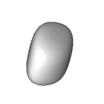
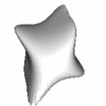
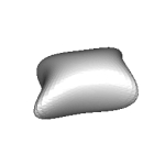
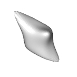
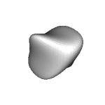
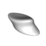
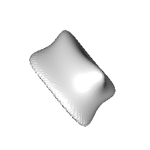
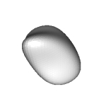
Figure 1: Constant surfaces of the determinant polynomials of tensors F$No1,3,10,20,99,119,207,237.$

Note that the numbering of tensors is based on the list of nonsingular tensors with elements consisting only of $-1,0,1$ found by us. Each figure corresponds to the following tensor and its determinant function respectively.

$$T_{1}=\left(\begin{array}[]{cccc}1&0&0&0\\ 0&1&0&0\\ 0&0&1&0\\ 0&0&0&1\\ \end{array}\right):\left(\begin{array}[]{cccc}-1&0&1&1\\ 1&-1&1&-1\\ -1&-1&-1&-1\\ 0&1&1&0\\ \end{array}\right):\left(\begin{array}[]{cccc}0&1&-1&1\\ 0&-1&1&1\\ 0&-1&0&-1\\ -1&-1&1&1\\ \end{array}\right),$$

$$f_{T_{1}}(x,y,z) = x^{4}+6y^{4}+2z^{4}+-3x^{3}y-8xy^{3}-3xz^{3}+5z^{3}y+$$

$$7x^{2}y^{2}+3x^{2}z^{2}+8z^{2}y^{2}-2xy^{2}z-8xyz^{2}.$$

$$T_{3}=\left(\begin{array}[]{cccc}1&0&0&0\\ 0&1&0&0\\ 0&0&1&0\\ 0&0&0&1\\ \end{array}\right):\left(\begin{array}[]{cccc}0&1&0&0\\ 0&-1&0&1\\ 1&0&-&0\\ -1&1&-1&1\\ \end{array}\right):\left(\begin{array}[]{cccc}1&1&1&1\\ -1&0&0&-1\\ 0&-1&0&0\\ -1&1&-1&1\\ \end{array}\right),$$

$$f_{T_{3}}(x,y,z) = x^{4}+3y^{4}+6z^{4}-3x^{3}z+2xy^{3}+4y^{3}z$$

$$-7xz^{3}-6z^{3}y+x^{2}y^{2}+5x^{2}z^{2}-5z^{2}y^{2}+4xy^{2}z-x^{2}yz+2xyz^{2}.$$

$$T_{10}=\left(\begin{array}[]{cccc}1&0&0&0\\ 0&1&0&0\\ 0&0&1&0\\ 0&0&0&1\\ \end{array}\right):\left(\begin{array}[]{cccc}0&1&0&0\\ 0&-1&0&1\\ 1&0&1&0\\ 0&0&-1&-1\\ \end{array}\right):\left(\begin{array}[]{cccc}1&1&1&1\\ -1&0&0&-1\\ 0&-1&0&0\\ -1&1&-1&1\\ \end{array}\right),$$

$$f_{T_{10}}(x,y,z)=x^{4}+y^{4}+2z^{4}-x^{3}y+2x^{3}z+xy^{3}+2xz^{3}$$

$$-z^{3}y-x^{2}y^{2}+4x^{2}z^{2}-2xy^{2}z-2x^{2}yz-xyz^{2}.$$

$$T_{20}=\left(\begin{array}[]{cccc}1&0&0&0\\ 0&1&0&0\\ 0&0&1&0\\ 0&0&0&1\\ \end{array}\right):\left(\begin{array}[]{cccc}-1&0&1&-1\\ 0&0&0&1\\ 1&-1&0&0\\ 1&0&0&0\\ \end{array}\right):\left(\begin{array}[]{cccc}1&0&1&1\\ 1&1&1&-1\\ 0&0&0&1\\ 1&-1&-1&-1\\ \end{array}\right),$$

$$f_{T_{20}}(x,y,z)=x^{4}+y^{4}+2z^{4}-x^{3}y+x^{3}z+y^{3}z-xz^{3}+2z^{3}y+$$

$$-x^{2}z^{2}+6z^{2}y^{2}+xy^{2}z+x^{2}yz+2xyz^{2}.$$

$$T_{99}=\left(\begin{array}[]{cccc}1&0&0&0\\ 0&1&0&0\\ 0&0&1&0\\ 0&0&0&1\\ \end{array}\right):\left(\begin{array}[]{cccc}0&-1&-1&-1\\ 1&1&1&-1\\ 1&-1&1&0\\ -1&1&-1&1\\ \end{array}\right):\left(\begin{array}[]{cccc}0&1&0&0\\ 0&-1&1&1\\ 1&0&1&-1\\ 1&0&1&1\\ \end{array}\right),$$

$$f_{T_{99}}(x,y,z)=x^{4}+2y^{4}+2z^{4}+3x^{3}y+x^{3}z+3xy^{3}+$$

$$y^{3}z-3z^{3}y+6x^{2}y^{2}+z^{2}y^{2}+8xy^{2}z+x^{2}yz-5xyz^{2}$$

$$T_{119}=\left(\begin{array}[]{cccc}1&0&0&0\\ 0&1&0&0\\ 0&0&1&0\\ 0&0&0&1\\ \end{array}\right):\left(\begin{array}[]{cccc}0&0&0&-1\\ -1&1&1&-1\\ 0&-1&0&0\\ 1&0&0&0\\ \end{array}\right):\left(\begin{array}[]{cccc}1&-1&-1&1\\ 1&-1&1&0\\ 0&1&1&1\\ 1&1&0&-1\\ \end{array}\right),$$

$$f_{T_{119}}(x,y,z)=x^{4}+y^{4}+9z^{4}+x^{3}y+xy^{3}+2y^{3}z-2z^{3}y+$$

$$2x^{2}y^{2}-3x^{2}z^{2}-z^{2}y^{2}+xy^{2}z+x^{2}yz+xyz^{2}.$$

$$T_{207}=\left(\begin{array}[]{cccc}1&0&0&0\\ 0&1&0&0\\ 0&0&1&0\\ 0&0&0&1\\ \end{array}\right):\left(\begin{array}[]{cccc}-1&-1&-1&1\\ 0&1&1&0\\ -1&0&0&-1\\ -1&1&0&-1\\ \end{array}\right):\left(\begin{array}[]{cccc}-1&1&-1&1\\ -1&0&1&1\\ -1&0&-1&1\\ 0&0&-1&-1\\ \end{array}\right),$$

$$f_{T_{207}}(x,y,z)=x^{4}+2y^{4}+2z^{4}-x^{3}y-3x^{3}z+xy^{3}+6y^{3}z$$

$$-3xz^{3}+2z^{3}y-x^{2}y^{2}+4x^{2}z^{2}+6z^{2}y^{2}+8xy^{2}z-3x^{2}yz+7xyz^{2}.$$

$$T_{237}=\left(\begin{array}[]{cccc}1&0&0&0\\ 0&1&0&0\\ 0&0&1&0\\ 0&0&0&1\\ \end{array}\right):\left(\begin{array}[]{cccc}0&-1&1&-1\\ 0&-1&-1&0\\ 0&1&-1&0\\ 1&1&0&1\\ \end{array}\right):\left(\begin{array}[]{cccc}0&-1&-1&-1\\ -1&-1&-1&0\\ 0&-1&0&1\\ 1&-1&1&1\\ \end{array}\right),$$

$$f_{T_{237}}(x,y,z)=x^{4}+2y^{4}+3z^{4}-x^{3}y+4y^{3}z+3z^{3}y+$$

$$x^{2}y^{2}-x^{2}z^{2}+6z^{2}y^{2}+x^{2}yz.$$

3 Notations from differential geometry

For the use in the following sections, we review some basic notations of differential geometry. For more details, for example, see the Nomizu and Sasaki [19]. When we denote the parametrized point on the surface by $x(s,t),$ we denote its partial derivatives by

$$x_{s}(s,t) = \frac{\partial x(s,t)}{\partial s},$$ (3.1)

$$x_{t}(s,t) = \frac{\partial x(s,t)}{\partial t}.$$ (3.2)

Definition 3.3

$$E=\langle x_{s},x_{s}\rangle,\ \ F=\langle x_{s},x_{t}\rangle,\ \ G=\langle x_{t},x_{t}\rangle,$$ (3.4)

are called the first fundamental coefficients. Putting $dx=x_{s}(s,t)ds+x_{t}(s,t)dt$, the form

$$I=\langle dx,dx\rangle=Es^{2}+2Mdsdt+Ndt^{2}$$ (3.5)

is called the first fundamental form of the surface.

Definition 3.6

$$\bm{n}=\frac{x_{s}\times x_{t}}{||x_{s}\times x_{t}||}$$ (3.7)

is called the unit normal vector at the point $x(s,t).$

Definition 3.8

Putting

$$x_{ss}=\frac{\partial^{2}x(s,t)}{\partial s^{2}},\ \ x_{ss}=\frac{\partial^{2}x(s,t)}{\partial st},\ \ x_{ss}=\frac{\partial^{2}x(s,t)}{\partial t^{2}},$$ (3.9)

the scalar functions

$$L=\langle x_{ss},\bm{n}\rangle\ \ M=\langle x_{st},\bm{n}\rangle\ \ \ \ N=\langle x_{tt},\bm{n}\rangle$$ (3.10)

are called the second fundamental coefficients. The form

$$II=-\langle dX,d\bm{n}\rangle=Lds^{2}+2Mdsdt+Ndt^{2}$$ (3.11)

is called the second fundamental form of the surface.

Definition 3.12

At the point $P$ on the surface, let $k_{1}$ and $k_{2}$ be the maximum and minimum of curvatures of curves generated by the intersection of the surface with the plane spanned by the normal vector and a tangent vector, $H=(k_{1}+k_{2})/2$ is called the mean curvature and $K=k_{1}k_{2}$ is called the Gaussian curvature. These are calculated by

$$H=\frac{EN-2FM+GL}{2(EG-F^{2})}\ \ {\rm and}\ \ K=\frac{LN-M^{2}}{EG-F^{2}}.$$ (3.13)

4 Rough $SL(3)$ invariants

For checking $GL(3)$-equivalence between two tensors $T_{1}$ and $T_{2}$, we need to test the equation

$$f_{T_{2}}(\bm{x})=cf_{T_{1}}(\bm{x}R),c\in\mathbb{R}\ \ {\rm and}\ \ R\in GL(3).$$

Further, $S=R/|R|^{1/3}\in SL(3),$

$$cf_{T_{1}}(\bm{x}R)=c|R|^{4/3}f_{T_{1}}(\bm{x}R/|R|^{1/3})=c^{\prime}f_{T_{1}}(\bm{x}S)\ \ with\ \ c^{\prime}\in\mathbb{R}\ \ and\ \ S\in SL(3).$$ (4.1)

Thus, $GL(3)$-equivalence reduces to $SL(3)$-equivalence. Then, the following theorem holds.

Theorem 4.2

For two tensors $T_{1}$ and $T_{2}$, assume that $f_{T_{2}}(\bm{x})=cf_{T_{1}}(\bm{x}S)$ does not hold for any choice of $c\in\mathbb{R}\ \ {\rm and}\ \ {\rm any}S\in SL(3)$. Then, $T_{1}$ and $T_{2}$ are not $GL(3)$ equivalent.

This justifies to study $SL(3)$-equivalence among absolutely nonsingular tensors for investigating $GL(3)$ equivalence.

Remark 4.3

If $c$ is negative, then by consider $T_{3}=PT_{2}$ with $|P|<0,$ we have

$$f_{T_{3}}(\bm{x})=cf_{T_{1}}(\bm{x}R),c\in\mathbb{R}^{+}\ \ {\rm and}\ \ R\in GL(3).$$

where $T_{3}$ is equivalent to $T_{2}.$ Thus, we can assume by writing $T_{3}$ as $T_{2}$ again

$$f_{T_{2}}(\bm{x})=cf_{T_{1}}(\bm{x}R),c\in\mathbb{R}^{+}\ \ {\rm and}\ \ R\in GL(3).$$

The following rough $SL(3)$ invariants are useful.

Theorem 4.4

A convex surface is transformed into a convex surface by a $SL(3)$ linear transformation and so, a tensor with a determinant polynomial whose constant surface is convex is not equivalent to a tensor with a determinant polynomial whose constant surface is not convex.

Only the tensor of No.1 has the convex surface among 8 figures in the Figure 1.1 and so the tensor of No. 1 is not $SL(3)$ equivalent to all other tensors in the Figure 1.

Definition 4.5

A point on the surface is called a singular point if the normal vector at the point can not be defined.

Theorem 4.6

If the constant surface of a tensor $T_{1}$ has a singular point and the constant surface of a tensor $T_{2}$ has no singular point, they are not $SL(3)$($GL(3))$ equivalent.

Example 4.7

Let

$$T_{1}=\left(\begin{array}[]{cccc}0&1&0&0\\ -1&0&0&0\\ 0&0&0&-1\\ 0&0&1&0\end{array}\right);\left(\begin{array}[]{cccc}0&0&1&0\\ 0&0&0&1\\ -1&0&0&0\\ 0&-1&0&0\end{array}\right);\left(\begin{array}[]{cccc}0&0&0&1\\ 0&0&-1&0\\ 0&1&0&0\\ -1&0&0&0\end{array}\right)$$

and

$$T_{2}=\left(\begin{array}[]{cccc}0&1&0&0\\ -1&0&0&0\\ 0&0&1&0\\ 0&0&0&1\\ \end{array}\right);\left(\begin{array}[]{cccc}0&0&0&-1\\ 0&0&1&0\\ 1&0&0&0\\ 0&1&0&0\\ \end{array}\right);\left(\begin{array}[]{cccc}0&0&1&0\\ 0&1&0&0\\ 0&0&0&1\\ 1&0&0&0\\ \end{array}\right),$$

and the determinant polynomials of $T_{1}$ and $T_{2}$ are given below respectively. Then, we have

$$f_{T_{1}}(x,y,z)=(x^{2}+y^{2}+z^{2})^{2},$$

and

$$f_{T_{2}}(x,y,z)=(x^{2}+y^{2})^{2}+z^{4}.$$

Note that both of them are positive definite, that is, both of $T_{1}$ and $T_{2}$ are absolutely nonsingular. It is clear that the constant surface of $f_{T_{1}}(\bm{x})$ is a sphere and it has no singular point, and on the other hand, that the constant surface of $f_{T_{2}}(\bm{x})$ is a conic and it has a singular point. Hence, $T_{1}$ and $T_{2}$ are not equivalent.

Definition 4.8

When we consider a mesh of the parameter space,it produces a lattice of points on the constant surface. Let $K_{+}$ be the number of lattice points at which the Gaussian curvature is positive, and $K_{-}$ and $K_{0}$ be defined in the same way.

Then we have

Theorem 4.9

The triplet $(K_{+},K_{-},K_{0})$ is an $SL(3)$-invariant.

5 $SL(3)$ integral invariants

The following Figure 2 and 3 shows the figures of convex bodies that are enclosed by constant surfaces. The number of figures corresponds to that in our list of absolutely nonsingular tensors( Maehara [18]).

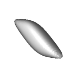
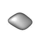
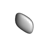
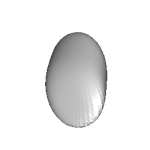
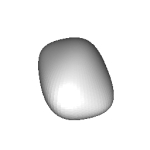
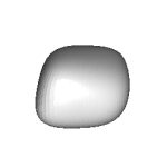
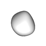
Figure 2: The constant surfaces for $No1,19,22,23,42,60,61,65$ absolutely nonsingular tensors

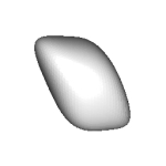
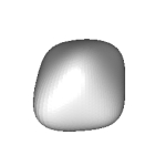
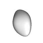
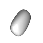
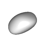
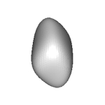
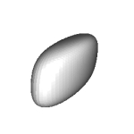
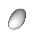
Figure 3: The constant surfaces for $No72,74,76,83,85,87,95,103$ absolutely nonsingular tensors

In this section, we want to find some $SL(3)$-invariant for such convex bodies. For this purpose, the following valuation theory is a quite useful. Here, we make a brief summary of the valuation theory from Ludwig [15] and [17]. The definition is stated for a general $p$.

Definition 5.1

Let $\mathcal{K}$ denote the set of all convex bodies in $\mathbb{R}^{p}$. A functional $t(\cdot)$ from $\mathcal{K}$ to $\mathbb{R}$ is called a valuation if it satisfies

$$t(K)+t(L)=t(K\cup L)+t(K\cap L),\ \ K,L\in\mathcal{K}.$$ (5.2)

Next theorem is a starting point of characterization of invariant valuation.

Theorem 5.3

(Hadwiger[9]). A continuous valuation $t(\cdot)$ from $\mathcal{K}$ to $\mathbb{R}$ is invariant with respect to rigid motion if and only if there are constants $c_{0},c_{1},...,c_{p}$ such that

$$t(K)=c_{0}V_{0}(K)+c_{1}V_{1}(K)+\cdots+c_{p}V_{p}(K),$$ (5.4)

where $V_{0}(K),V_{1}(K),\cdots,$ and $V_{p}(K)$ are the intrinsic volumes of $K.$ We remark that the volumes $V_{k}$ are called quermassintegrals of $K$ in [13] and that $V_{0}$ is the Euler index, $V_{p-1}$ the affine volume of $\partial K$, and $V_{p}$ is the volume of the convex body $K.$ In the following, we simply denote by $a(K)$ as the affine volume and call it affine surface area following [17], and denoe by $V(K)$ the volume $V_{p}(K)$.

Definition 5.5

A functional $t(\cdot)$ on $\mathcal{K}$ is said to be equi-affine invariant if it is $SL(p)$-invariant and location invariant.

The following is essential for us.

Theorem 5.6

(Ludwig [14] ,[16], [15] and [17] ). An upper semi-continuous valuation $t(K)$ from $\mathcal{K}$ to $\mathbb{R}$ is equi-affine invariant if and only if there are constants $c_{0},c_{1},\in R$ and $c_{2}\geq 0$ such that

$$t(K)=c_{0}V_{0}(K)+c_{1}V_{p}(K)+c_{2}a(K),$$ (5.7)

where $a(K)$ denotes the affine surface area.

In short, $SL(p)$ invariant valuation is only the weighted sum of the Euler index and the volume $V_{p}(K)$and the affine surface area $a(K)$. This means that

Proposition 5.8

$V(K)$ and $a(K)$ are $SL$-invariants.

So, we adopt the volume $V(K)$ and the affine surface area $a(K)$ as indexes of $SL(p)$-equivalence. Further, the next proposition by Lutwak[20] is very useful for us.

Proposition 5.9

When $p=3$,$a(K)$is homogeneous of degree $3/2$, that is,

$$a(dK)=d^{3/2}a(K),K\in\mathcal{K}_{0}.$$ (5.10)

5.1 Volume as an $SL(3)$-invariant

We are considering the equivalence relation among absolutely nonsingular tensors. As is shown in Theorem 2.7, for such kind of tensors, the constant surfaces of them are compact. Note that from Propisition 5.8 the volume of the region enclosed by the constant surface is $SL(3)$-invariant. Then, by the following Gauss’s theorem, we can calculate the volume by the parametric representation given by the equation (2.6).

Theorem 5.11

(Gaussian formula)
For the region $\Omega$ enclosed by the space surface $\partial\Omega$, letting $fdy\wedge dz+gdz\wedge dx+hdx\wedge dy$ be the differential form of 2nd degree, it holds

$$\int_{\partial\Omega}fdy\wedge dz+gdz\wedge dx+hdx\wedge dy=\int_{\Omega}\left(\frac{\partial f}{\partial x}+\frac{\partial g}{\partial y}+\frac{\partial h}{\partial z}\right)dx\wedge dy\wedge dz$$ (5.12)

We denote by $V(\Omega)$ the volume of the region $\Omega$. By this formula, we have

$$V(\Omega)=LHS\ \ of\ \ the\ \ equation(\ref{Gauss}).$$ (5.13)

For the present case, by use of the spherical coordinates (s,t), the point of the boundary $\partial\Omega$ is parametrized as $\bm{x}=r(s,t)(\Phi_{x}(s,t),\Phi_{y}(s,t),\Phi_{z}(s,t)).$ Hence, we have

$$dy = \frac{\partial y}{\partial s}ds+\frac{\partial y}{\partial t}dt$$

$$= \left((-1/4)\frac{dp/ds}{p^{5/4}}\Phi_{y}+\frac{d\Phi_{y}/ds}{p^{1/4}}\right)ds+$$

$$\left((-1/4)\frac{dp/dt}{p^{5/4}}\Phi_{y}+\frac{\Phi_{y}/dt}{p^{1/4}}\right)dt$$

$$dz = \frac{\partial z}{\partial s}ds+\frac{\partial z}{\partial t}dt,$$

$$= \left((-1/4)\frac{dp/ds}{p^{5/4}}\Phi_{z}+\frac{d\Phi_{z}/ds}{p^{1/4}}\right)ds+$$

$$\left((-1/4)\frac{dp/dt}{p^{5/4}}\Phi_{z}+\frac{\Phi_{z}/dt}{p^{1/4}}\right)dt.$$

Therefore,

$$dy\wedge dz = \left((-1/4)\frac{dp/ds}{p^{5/4}}\Phi_{y}+\frac{d\Phi_{y}/ds}{p^{1/4}}\right)\left((-1/4)\frac{dp/dt}{p^{5/4}}\Phi_{z}+\frac{\Phi_{z}/dt}{p^{1/4}}\right)ds\wedge dt$$

$$-\left((-1/4)\frac{dp/dt}{p^{5/4}}\Phi_{y}+\frac{\Phi_{y}/dt}{p^{1/4}}\right)\left((-1/4)\frac{dp/ds}{p^{5/4}}\Phi_{z}+\frac{d\Phi_{z}/ds}{p^{1/4}}\right)ds\wedge dt.$$

Similarly,

$$dz\wedge dx = \left((-1/4)\frac{dp/ds}{p^{5/4}}\Phi_{z}+\frac{d\Phi_{z}/ds}{p^{1/4}}\right)\left((-1/4)\frac{dp/dt}{p^{5/4}}\Phi_{x}+\frac{\Phi_{x}/dt}{p^{1/4}}\right)ds\wedge dt$$

$$-\left((-1/4)\frac{dp/dt}{p^{5/4}}\Phi_{z}+\frac{\Phi_{z}/dt}{p^{1/4}}\right)\left((-1/4)\frac{dp/ds}{p^{5/4}}\Phi_{x}+\frac{d\Phi_{x}/ds}{p^{1/4}}\right)ds\wedge dt,$$

and

$$dx\wedge dy = \left((-1/4)\frac{dp/ds}{p^{5/4}}\Phi_{x}+\frac{d\Phi_{x}/ds}{p^{1/4}}\right)\left((-1/4)\frac{dp/dt}{p^{5/4}}\Phi_{y}+\frac{\Phi_{y}/dt}{p^{1/4}}\right)ds\wedge dt$$

$$-\left((-1/4)\frac{dp/dt}{p^{5/4}}\Phi_{x}+\frac{\Phi_{x}/dt}{p^{1/4}}\right)\left((-1/4)\frac{dp/ds}{p^{5/4}}\Phi_{y}+\frac{d\Phi_{y}/ds}{p^{1/4}}\right)ds\wedge dt.$$

By using these, we can calculate the volume of the region enclosed by the constant surface of the determinant polynomial. Let $T_{1}$ and $T_{2}$ be two $n\times n\times 3$ tensors and let $\Omega_{i}$ denote the regions $\{\\ bm{x}|f_{T_{i}}(\bm{x})\leq 1\}$, which are enclosed by the surfaces of $\{\bm{x}|f_{T_{1}}(\bm{x})=1\}$. Then, by $SL(3)$ invariance of volumes, we have

Theorem 5.16

If $V_{1}\neq V_{2},$ $f_{T_{2}}(\bm{x})\neq f_{T_{1}}(\bm{x}R)$ for any $R\in SL(3)$, namely, $T_{1}$ and $T_{2}$ are not $SL(n)\times SL(n)\times SL(3)$ equivalent.

For $GL$ invariance, the next lemma is helpful.

Lemma 5.17

For a determinant polynomial $f(\bm{x}),$ let $V(c)$ be the volume of $\Omega_{c}=\{\bm{x}|cf(\bm{x})\leq 1\}.$ Then $V(c)=c^{-3/4}V(1)$ for $4\times 4\times 3$ case.

Proof  By changing a polynomial $f(\bm{x})$ into its constant multiple $cf(\bm{x})$, the coordinates $\bm{x}(s,t)$ on the constant surface are subject to changes to $(\frac{1}{c})^{1/4}\bm{x}(s,t)$. Hence, the integral

$$\frac{1}{3}\int_{\partial\Omega}xdy\wedge dz+ydz\wedge dx+zdx\wedge dy$$ (5.18)

is multiplied by $c^{-3/4}.$ This proves the assertion of Lemma 5.17.  

Theorem 5.19

Assume that $T_{1}$ and $T_{2}$ be $SL(3)$ equivalent and therefore that there is a relation between their determinant polynomials,

$$f_{T_{2}}(\bm{x})=cf_{T_{1}}(\bm{x}R),$$ (5.20)

where $c\in\mathbb{R}$ and $R\in SL(3)$. Let $V_{1}(c)$ and $V_{2}(c)$ denote the volumes of $\Omega^{(1)}_{c}=\{\bm{x}|cf_{T_{1}}(\bm{x})\leq 1\}$ and $\Omega^{(2)}_{c}=\{\bm{x}|cf_{T_{2}}(\bm{x})\leq 1\}$ respectively. Then, it holds that

$$c=(V_{1}/V_{2})^{4/3}.$$ (5.21)

Proof  The proof is trivial from Lemma 5.17 and omitted.  

From Theorem 5.19, we can know the constant $c$ in the equation (5.20). In the next section, it will be made clear that this expresson is helpful for establishing $GL(3)$-equivalence.

5.2 Affine surface area as an $SL(3)$-invariant

In this section, for testing $SL(3)$-equivalence, we propose to use the affine surface area, which is an $SL(3)$-invariant by Theorem 5.8. When $p=3$, the affine surface area has the following integral expression.

Definition 5.22

For a smooth convex body $K\subset\mathbb{R}^{3}$, the affine surface area is given by

$$a(K)=\int_{\partial K}\kappa(K,\bm{x})^{\frac{1}{4}}\sqrt{EG-F^{2}}dsdt,$$ (5.23)

where $\kappa(\partial K,\bm{x})$ is the Gaussian curvature and $E,F$ and $G$ denote the first fundamental coefficients.

Next, we show that the affine surface area is useful even as a tester of $GL(3)$-equivalence. Assume that we know the constant $c$ in the relation $f_{T_{2}}(\bm{x})=cf_{T_{1}}(\bm{x}R)$ with $c\in\mathbb{R}^{+}$ and $R\in SL(3)$ by Theorem 5.19. Then,

$$\Omega_{2} = \{\bm{x}|f_{T_{2}}(\bm{x})\leq 1\}$$

$$= \{\bm{x}|cf_{T_{1}}(\bm{x})\leq 1\}$$

$$= \{\bm{x}|f_{T_{1}}(c^{1/4}\bm{x})\leq 1\}$$

$$= c^{-1/4}\{\bm{x}|f_{T_{1}}(\bm{x})\leq 1\}$$

$$= c^{-1/4}\Omega_{1}.$$

From Proposition 5.9, we have

$$a(\Omega_{2})=c^{-3/8}a(\Omega_{1}).$$ (5.26)

Thus, we have the following.

Theorem 5.27

Let $T_{1}$ and $T_{2}$ be absolutely nonsingular tensors. Noting Remark 4.3, by Theorem 5.19, we can obtain the estimate of $c\in R^{+}$ under the assumption that their determinant polynomials have the relation $f_{T_{2}}(\bm{x})=cf_{T_{1}}(\bm{x}R)$ for some unknown constant $c\in\mathbb{R}^{+}$ and an unknown matrix $R\in SL(3).$ Then, if $a(\Omega_{2})\neq c^{-1/8}a(\Omega_{1})$, $T_{1}$ and $T_{2}$ are not $GL(3)$ equivalent.

By using Theorem 5.17, this is rephrased as

Theorem 5.28

Let $T_{1}$ and $T_{2}$ be absolutely nonsingular tensors. Then, if

$$a(\Omega_{2})\neq\left(\frac{V(\Omega_{2})}{V(\Omega_{1})}\right)^{1/2}a(\Omega_{1}),$$ (5.29)

$T_{1}$ and $T_{2}$ are not $GL(3)$-equivalent, where $V(\Omega_{1})$ and $V(\Omega_{2})$ denote the volume of $\Omega_{1}$ and $\Omega_{2}$ respectively.

6 Integral $GL(3)$-invariant

In the latter half of the previous section, we presented a procedure to test a non-$GL(3)$-equivalence, however, it is somewhat indirect because we need to estimate the constant $c$ before starting the procedure. In this section, we consider a direct method handling non-equivalence by using a generalized affine surface area. That is, we consider the $L_{q}$ affine surface area, which is an extension of the affine surface area and developed by Letwak [20]. Hug [10] gave an equivalent definition. The following is the Hug’ s definition.

Definition 6.1

$$L_{q}a(K)=\int_{\partial K}\kappa_{0}(K,\bm{x})^{\frac{q}{p+q}}d\sigma_{K}(\bm{x})$$ (6.2)

where

$$\kappa_{0}(K,\bm{x})=\frac{\kappa(K,\bm{x})}{\langle\bm{x},\bm{n}(K,\bm{x})\rangle^{p+1}}.$$ (6.3)

and $d\sigma_{K}(\bm{x})$ is called a cone measure defined by

$$d\sigma_{K}(\bm{x})=\langle\bm{x},\bm{n}(K,\bm{x})\rangle d\bm{x},$$ (6.4)

and $\bm{n}(K,\bm{x})$ denotes the outer normal at $\bm{x}$ on $\partial K.$

When $q=1$, $L_{q}(K)$ becomes the affine surface area $a(K)$, and when $q=p$, it becomes a classical centro-affine surface area $a_{c}(K)$ thta is defined as

$$a_{c}(K)=\int_{\partial K}\kappa_{0}(K,\bm{x})^{1/2}d\sigma_{K}(\bm{x}),$$ (6.5)

which is known to be $GL(p)$-invariant. The characterization of a general $GL(p)$-invariant functional is given below.

Theorem 6.6

(Ludwig and Reitzsner [17] ) Let $\mathcal{K}_{0}$ be the space of convex bodies that contain the origin in their interiors. An upper semi-continuous functional $t(\cdot)$ from $\mathcal{K}_{0}$ to $\mathbb{R}^{1}$ is $GL(p)$-invariant if and only if there are nonengative constants $c_{0}$ and $c_{1}$ such that

$$t(K)=c_{0}V_{0}(K)+c_{1}a_{c}(K).$$ (6.7)

7 Spherical design

According to our experiments, the numerical integrations of the invariants must be accurate at least 2 decimals. So, the caluculations of the invariants are a little bit heavy. In this section, we consider the t-design method as an substitute of the nemerical integrations. The spherical design was initiated by Delsarte et al. [7] and has been studied by several researchers, for example, see Bannai and Bannai [3]. It is defined as follows.

7.1 An overview of spherical design

Definition 7.1

A finite set $X$ on the sphere is called t-spherical design if the following equality holds that for any polynomial $f(x,y,z)$ with a degree less than or equal to $t,$

$$\frac{1}{|S^{2}|}\int_{S^{2}}f(x,y,z)d\sigma=\frac{1}{|X|}\sum_{(x,y,z)\in X}f(x,y,z),$$ (7.2)

where $S^{2}$ denotes the unit sphere of $\mathbb{R}^{3}$ and $d\sigma$denotes the surface element of the sphere and $|S^{2}|$ denotes the surface area of the sphere.

A parametrized integral formula of the equation 7.2 is given by

$$\int f(s,t)\sin(s)dsdt=\frac{4\pi}{N}\sum_{i=1}^{N}f(s_{i},t_{i}),$$ (7.3)

where $(s_{i},t_{i}),i=1,2,....,N$ are the corresponding parameters to the design points in $X$. One point to overcome for our purpose is that we need to integrate some nonlinear functions that are not polynomials and hence we can not use any t-design directly. However, we can rely on the next theorem to solve this point.

Theorem 7.4

Let $f(x,y,z)$ be an continuous function over the unit sphere and let $\epsilon_{t}$ be a positive number such that

$$|f(x,y,z)-p(x,y,z)|<\epsilon_{t}$$

uniformly for some polynomial $p(x,y,z)$ with degree less than or equal to $t$. Then, it holds that

$$|\int_{\partial S}f(x,y,z)dS-4\pi\frac{1}{N}\sum_{i=1}^{N}f(x_{i})|<8\pi\epsilon_{t}$$ (7.5)

Proof

$$\left|\int_{\partial S}f(x,y,z)dS-4\pi\frac{1}{N}\sum_{i=1}^{N}f(x_{i})\right|$$

$$\leq \left|\int_{\partial S}f(x,y,z)dS-4\pi\frac{1}{N}\sum_{i=1}^{N}p(x_{i})\right|+\left|4\pi\frac{1}{N}\sum_{i=1}^{N}p(x_{i})-4\pi\frac{1}{N}\sum_{i=1}^{N}f(x_{i})\right|$$

$$= \left|\int_{\partial S}f(x,y,z)dS-\int_{|\partial S}p(x_{i})dS\right|+\frac{4\pi}{N}\left|\sum_{i=1}^{N}|p(x_{i})-f(x_{i})|\right|$$

$$\leq \int\epsilon_{t}dS+4\pi\epsilon_{t}$$

$$= 8\pi\epsilon_{t}$$

 

Remark 7.7

By the above theorem, we need not to know the best approximate polynomial concretely in order to obtain an approximate value of the integration, and it is enough to use $f(x,y,z)$ itself. Moreover the error of the approximation is bounded from above by the multiple of $\epsilon_{t}$ by $8\pi.$ For a substantial evaluation of the approximation, we need to know $\epsilon_{t}$. The problem is interesting, however, it is a little bit heavy task at present, and so it is postponed to the future work.

7.2 Calculation of integral invariants by a 20-design

Using the result of the previous subsection, we consider the integration

$$a(K)=\int\kappa(s,t)^{1/4}\sqrt{EG-F^{2}}dsdt.$$ (7.8)

where $s,t$ moves $0<s<\pi$,$0<t<2\pi$. This integration can be thought to be an integration over the unit sphere by

$$a(K) = \int_{(s,t,)\in[0,\pi]\times[0,2\pi]}\kappa(s,t)^{1/4}\sqrt{EG-F^{2}}dsdt$$

$$= \int_{(s,t,)\in[0,\pi]\times[0,2\pi]}\kappa(s,t)^{1/4}\frac{\sqrt{EG-F^{2}}}{\sin s}\sin sdsdt$$

$$= \int_{\partial S}\kappa(s,t)^{1/4}\frac{\sqrt{EG-F^{2}}}{\sin s}dS,$$

where $dS=sin(s)$. Hence,

$$p(x,y,z)=\kappa(s,t)^{1/4}\frac{\sqrt{EG-F^{2}}}{\sin s}$$ (7.11)

is taken to be a function over the unit sphere and so the integral invariant can be approximated by the right hand side of the equation below.

$$\int_{\partial S}\kappa(s,t)^{1/4}\frac{\sqrt{EG-F^{2}}}{\sin s}dS\sim\frac{4\pi}{N}\sum_{i=1}^{N}p(x_{i},y_{i},z_{i})$$ (7.12)

The values of invariants calculated by the lattice method and the 20-design method will be give in the next section. The 20-design method show very nice approximations in some cases, however, do not show good approximations for other cases. That is, for our integration of invariants, the spherical design method does not give stable values, unfortunately. This might suggest that we need to use design with more higher degree than 20.

8 Effectiveness of the invariants as testers of non-equivalence

In this section, we will show the effectiveness of the numerical values of the invariants as testers of non-equivalence. We numerically calculated the volume $V(\Omega)$, the affine surface area $a(\Omega)$and centro-affine surface area $a_{c}(\Omega)$ of the region $\Omega=\{\bm{x}|f(\bm{x}\leq 1\}$ defined by the determinant polynomials $f_{T}(\bm{x})$. As examples, we calculate them for the 16 tensors which are in $\mathcal{K}_{0}$, whose constant surfaces are figured in Figures 2 and 3 in the section 5. The numerical calculations are performed in two way, that is, by the lattice method and by the t-design method, and they are compared. As for the t-design method, we use the 20-design named des.3.216.20 in [8] which has 216 points. In the tables below, M1-P2-G5, M6-P2-G, M1-P2-G7 and 20-design denote the globally adaptive integration with accuracy of 5 digits, pseudo-Monte Carlo integration, the globally adaptive integration with accuracy of 7 digits by 64 decimal calculation and 20-design method by IEEE754 decimal calculation, respectively. For all calculation were done by Mathematica.

Tensor	V0	V1	V2	V3
T001	2.9197794095194	2.9197794099529	2.9197794089308	2.9197794061274
T019	4.0314824331814	4.0314824340674	4.0314824332515	4.0314824319603
T022	3.6306602017309	3.6306602004447	3.6306602054741	3.6306602016552
T023	3.4355628950802	3.4355628819358	3.4355628878857	3.4355628897838
T042	3.7515624235646	3.7515624142272	3.7515624197586	3.7515624152774
T060	2.1440485535226	2.1440485507771	2.1440485551454	2.1440485550215
T061	2.8594583429857	2.8594583441125	2.8594583445567	2.8594583445567
T065	3.1084258968340	3.1084258946417	3.1084258957994	3.1084258984271
T072	4.6861403575076	4.6861403597489	4.6861403542060	4.6861403560079
T074	3.6302252513670	3.6302253269919	3.63022533280632	3.6302253350968

Table 1: Volumes by M1-P2-G7 :$Tn$, where $n=001,0019,022,023,042,060,061$, $065,072$ and $074$ Each line denoted as $T$n-0 lists the value of the original tensor and the lines $T$n-i,$i=1,2,...,5$ list the values for the transformed tensors of Tn by a randomly chosen matrix of $SL(3)$.

Tensor	M1-P2-G5	M6-P2-G5	M1-P2-G7	20-design
T001-0	9.961493457	9.962796404	9.961471493	9.90317
T001-1	9.961470358	9.961249135	9.961471489	8.73023
T001-2	9.961471133	9.971266750	9.961471486	9.96328
T001-3	9.961470327	9.959509709	9.961471474	9.79057
T001-4	9.961471186	9.979456186	9.961471478	10.88367
T001-5	9.961474220	9.997180989	9.961471490	10.99278
T019-0	11.560007113	11.560055546	11.560007991	11.87277
T019-1	11.560007742	11.552017302	11.560007993	11.69239
T019-2	11.560008558	11.559866424	11.560007993	11.51344
T019-3	11.560007692	11.501609971	11.560007989	13.36769
T019-4	11.560008494	11.545260017	11.560007991	10.40203
T019-5	11.560001924	11.558176522	11.560007996	11.49393
T022-0	11.020675684	11.024551464	11.020674135	11.05202
T022-1	11.020673831	11.016947424	11.020674138	11.45345
T022-2	11.020676195	11.027525350	11.020674147	11.54386
T022-3	11.020673214	11.016006939	11.020674140	11.07524
T022-4	11.020675399	11.031596952	11.020674133	11.37096
T022-5	11.020674431	11.022431931	11.020674135	10.74089
T023-0	10.771760482	10.773095422	10.771760351	10.73293
T023-1	10.771758801	10.774759865	10.771760349	9.26881
T023-2	10.771759301	10.725843291	10.771760352	10.94587
T023-3	10.771759730	10.766135806	10.771760352	13.23848
T023-4	10.771757516	10.773059224	10.771760350	10.78732
T023-5	10.771759533	10.773749461	10.771760351	10.88149
T042-0	11.136697741	11.136755128	11.136697332	10.99424
T042-1	11.136695637	11.140565725	11.136697314	11.28015
T042-2	11.136699257	11.140835239	11.136697323	11.89052
T042-3	11.136721676	11.203272583	11.136697308	12.13058
T042-4	11.136696147	11.106329119	11.136697270	9.81007
T042-5	11.136697731	11.107102150	11.136697313	13.99432

Table 2: Affine surface area:$Tn$, where $n=001,019,022,023$ and $042$ Each line denoted as $T$n-0 lists the value of the original tensor and the lines $T$n-i,$i=1,2,...,5$ list the values for the transformed tensors of Tn by a randomly chosen matrix of $SL(3)$.

Tensor	M1-P2-G5	M6-P2-G5	M1-P2-G7	20-design
T060-0	8.704587985	8.705126156	8.704588101	8.74300
T060-1	8.704590255	8.781085267	8.704588109	8.50058
T060-2	8.704596276	8.705498658	8.704588101	8.73210
T060-3	8.704588380	8.711001740	8.704588104	8.80910
T060-4	8.704586669	8.703029024	8.704587984	8.85973
T060-5	8.704588143	8.705901809	8.704588100	8.56701
T061-0	9.759043314	9.759635865	9.759045706	9.741275
T061-1	9.759036154	9.759076500	9.759045704	9.72403
T061-2	9.759050068	9.748685352	9.759045707	9.56041
T061-3	9.759044653	9.734392909	9.759045710	9.76040
T061-4	9.759058206	9.745677922	9.759045694	10.37056
T061-5	9.759046974	9.755984062	9.759045716	8.72501
T065-0	10.273389075	10.274251947	10.273389369	10.33927
T065-1	10.273387633	10.260497042	10.273389360	10.76367
T065-2	10.273389342	10.277789370	10.273389368	10.26620
T065-3	10.273388029	10.249526640	10.273389366	10.42661
T065-4	10.273389939	10.276245030	10.273389370	10.06295
T065-5	10.273397527	10.279052599	10.273389365	10.33636
T072-0	12.483701912	12.483843205	12.483691274	12.67586
T072-1	12.483689616	12.484388161	12.483691282	12.38965
T072-2	12.483690234	12.481034408	12.483691282	10.30731
T072-3	12.483690116	12.498107747	12.483691264	11.96858
T072-4	12.483698348	12.435166726	12.483691276	11.219584
T072-5	12.483686195	12.508162438	12.483691276	10.183837
T074-0	10.732327625	10.732623087	10.732332110	10.80078
T074-1	10.732332283	10.726775221	10.732332117	10.55820
T074-2	10.732337739	10.734008328	10.732332113	11.20578
T074-3	10.732332889	10.724453313	10.732332112	10.87848
T074-4	10.732331733	10.729148909	10.732332214	10.95073
T074-5	10.732329467	10.727707310	10.732332111	10.57017

Table 3: Affine surface area:$Tn$, where $n=060,061,065,072$ and $074$ Each line denoted as $T$n-0 lists the value of the original tensor and the lines $T$n-i,$i=1,2,...,5$ list the values for the transformed tensors of Tn by a randomly chosen matrix of $SL(3)$.

Table 1 shows that the SL invariance of volumes of the redions enclosed by the constant surface is clealry seen numerically for every absolutely nonsingular chosen tensors. Tables 2 and 3 of the affine surface area show that the affine suraface area is SL invariant and that all relevant tensors are not $SL(4)\times SL(4)\times SL(3)$ equivalent mutually. From Theorem 5.28, combining the volume data, we also conclude that they are not $GL$ equivalent. This last fact is also derived by a direct usage of the centro-affine surface data which is seen in Table 4 and Table 5.

Tensor	M1-P2-G7	M6-P2-G5	M1-P2-G5	20-design
T001-0	11.690150892617500	11.687899476332365	11.687898336789288	11.59968
T001-1	11.751922920525157	11.687898955213611	11.687898343722015	8.421025
T001-2	11.689694693901319	11.687898370365255	11.687898355824357	11.68469
T001-3	11.721355953709315	11.687894829195568	11.687898343333765	11.29880
T001-4	11.692877418652227	11.687897242831659	11.687897875631138	10.59083
T001-5	11.679997753276740	11.687897167430656	11.687898359334835	11.46900
T019-0	11.509733354093680	11.509334536488204	11.509333804897551	11.81248
T019-1	11.472821548199051	11.509332873485376	11.509333807975230	12.65290
T019-2	11.509963231209824	11.509337447098934	11.509333799194381	11.32764
T019-3	11.552527050941017	11.509334159193976	11.509333800434498	11.38444
T019-4	11.495864684062547	11.509335287391230	11.509333801132503	11.37034
T019-5	11.522546264759133	11.509333512497239	11.509333798526679	22.50564
T022-0	11.574282949497377	11.568790730790213	11.568790156808308	11.59771
T022-1	11.570887655990263	11.568785645774059	11.568790144452251	11.63356
T022-2	11.568787229271756	11.568788230429048	11.568790347476747	11.90185
T022-3	11.567926875696718	11.568789765657722	11.568790134358534	11.57677
T022-4	11.597381830882211	11.568789372237021	11.568790132199215	13.39389
T022-5	11.561310960443544	11.568790290463560	11.568790451975676	11.44911
T023-0	11.631078897689606	11.626439742081966	11.626439153758515	11.57877
T023-1	11.619997976153462	11.626439518693340	11.626439146934238	11.39835
T023-2	11.611266008293132	11.626440231360507	11.626439154231153	11.43501
T023-3	11.647477652583963	11.626433368429471	11.626439151521914	13.20628
T023-4	11.607565993095791	11.626439544654837	11.626439154062155	10.72795
T023-5	11.620421522261536	11.626439658214246	11.626439152653352	11.74869
T042-0	11.502624357421948	11.504755263366923	11.504752079092657	11.30545
T042-1	11.507105268508006	11.504753311150279	11.504752086650519	11.07124
T042-2	11.519424921951189	11.504753899401661	11.504752079220612	9.41924
T042-3	11.501095106227783	11.504764044950799	11.504752085646500	12.16150
T042-4	11.530791206130419	11.504752412140897	11.504752073761618	10.11515
T042-5	11.499503647742464	11.504752956532382	11.504752076792938	10.64605

Table 4: Centro-affine surface area:$Tn$, where $n=001,019,022,023$ and $042$ Each line denoted as $T$n-0 lists the value of the original tensor and the lines $T$n-i,$i=1,2,...,5$ list the values for the transformed tensors of Tn by a randomly chosen matrix of $GL(3)$.

Tensor	M6-P2-G5	M1-P2-G5	M1-P2-G7	20-design
T060-0	11.989971644000403	11.989476119401702	11.989477685702977	12.05017
T060-1	11.990418566344240	11.989479611584825	11.989477723348062	12.01483
T060-2	11.976852295964006	11.989478648296963	11.989477738864300	11.80414
T060-3	11.994778478025750	11.989477993940143	11.989477740049253	11.64148
T060-4	11.989039776987073	11.989478217916079	11.989477724638414	12.09719
T060-5	12.046738095770048	11.989477160425962	11.989477721024015	12.11083
T061-0	11.519673795399891	11.518135424201142	11.518135117247486	11.48023
T061-1	11.518661618867961	11.518134427948641	11.518135113069415	11.45852
T061-2	11.519323023325257	11.518135433182912	11.518135109619174	11.45517
T061-3	11.517878708284445	11.518130456996306	11.518135109891727	11.66299
T061-4	11.517606307852915	11.518129721219993	11.518135107795112	11.47192
T061-5	11.531441863084249	11.518134741001642	11.518135110921667	10.31802
T065-0	11.660951650838694	11.660077139783777	11.660146606151409	11.77330
T065-1	11.657097464096733	11.660146835636129	11.660146583158155	11.64542
T065-2	11.662671583310311	11.660135616613492	11.660146602669996	11.69570
T065-3	11.657074111599187	11.660148534680922	11.660146593520388	11.58150
T065-4	11.661605706427124	11.660146860738219	11.660146601870989	12.45337
T065-5	11.668831112582931	11.660147254608734	11.660146596730511	11.76209
T072-0	11.545589518947570	11.545142097769179	11.545141226929544	11.76647
T072-1	11.545716622630585	11.545139592226001	11.545141221483210	11.52675
T072-2	11.562200209044268	11.545142319259361	11.545141224116661	8.50885
T072-3	11.575704218963165	11.545144648175810	11.545141226744587	10.30769
T072-4	11.535076590703719	11.545140326506765	11.545141235723655	12.22675
T072-5	11.545910129113601	11.545141536682674	11.545141208615009	11.19618
T074-0	11.116314213623787	11.116088526600165	11.116090556639371	11.20632
T074-1	11.109183432623630	11.116086365050504	11.116090553382580	11.09112
T074-2	11.121063605466493	11.116094135711593	11.116090554260284	9.58706
T074-3	11.090134159234779	11.116089713933696	11.116090550551305	10.19594
T074-4	11.135697898280837	11.116091869446610	11.116090554811293	11.15140
T074-5	11.117481923868303	11.116094503240262	11.116090554606608	11.08749

Table 5: Centro-affine surface area:$Tn$, where $n=060,061,065,072$ and $074$ Each line denoted as $T$n-0 lists the value of the original tensor and the lines $T$n-i,$i=1,2,...,5$ list the values for the transformed tensors of Tn by a randomly chosen matrix of $GL(3)$.

Indeed, Tables 4 and 5 show that the centro-affine surface area is really $GL$ invarinat, and that three point decimal accuracy will be sufficient to detect non $GL(3)$-equivalence between $4\times 4\times 3$ absolutely nonsingular tensors, whose elements consists of only -1,0,1. The M1-P2-G7 method seems clearly the best for discriminating the tensors relating to $GL$ nonequivalence.

9 Conclusion

We treated the $SL(4)\times SL(4)\times SL(3),$ $GL(4)\times GL(4)\times SL(3)$ or $GL(4)\times GL(4)\times GL(3)$ non-equivalence problem of $4\times 4\times 3$ absolutely nonsingular tensors. We proposed a method to addres to the problem through the determinant polynomials. Furthermore we proposed to solve the problem by differential geometric $SL(3)$ or $GL(3)$ invariant of the constant surface of the determinant polynomials. From the numerical analysis by Mathematica, it was shown that the stable values of invariants are obtainable numerically and also it was shown that the affine surface area and the centro-affine surface area are useful to detect the non-equivalence. This means that the algebraic problem: whether a system of algebraic equations with many variables can have real solutions or not, can be resolved by differential geometric methods. It is a nice link between algebra and differential geometry. Second, we investigated the spherical design method for calculating invariants. At present, we think that the values given by the adaptive lattice methods are more reliable than those given by the spherical design method. In some future work, we expect to extend the result to more higher dimensional tensors and to know why the spherical design method does not give stable values of invariants.

References

- [1] M.D. Atkinson and S. Lloyd, Bounds on the ranks of some -tensors, Linear Algebra and its applications 31 (1980), 19–31.
- [2] M. D. Atkinson and M. Stephens, On the maximal multiplicative complexity of a family of bilinear forms, Linear Algebra and its applications 27 (1979),1–8.
- [3] E. Bannai and E. Bannai, A survey of spherical designs and algebraic combinatorics on spheres. Europian J. of Combinatorics,30 (2009),1392–1425.
- [4] W. Blaschke, Vorlesungen über Differential geometrie II, Springer Verlag, Berlin 1923.
- [5] L. Chen, Yi. Chen and Y. Mei, Classification of multipartite entanglement containing infinitely many kinds of states, Phys. Revs. A 74 (2006), no. 5, 052331, 1–12.
- [6] P. Comon, J.M.F. ten Berge, L.D. Lathauwer and J. Castaing, Generic and typical ranks of multi-way arrays, Linear Algebra Applications 430 (2009), no. 11-12, 2997–3007.
- [7] P. Delsarte, J.M. Goethals and J.J Seidel, Spherical codes and designs, Geom. Dedicata 6 (1977), 363–388.
-
[8]
R. H. Hardin and Sloane, N.J.A., Spherical Designs
http://www2.research.att.com/ njas/sphdesigns/dim3/. - [9] H. Hadwiger, Vorlesungen ber Inhalt, Oberflshe und Isoperimetrie, Springer, Berlin,1957.
- [10] D. Hug, Contributions to affine surface area, manuscripta mathematics 91 (1996), 283–301.
- [11] T.G. Kolda and B.W, Bader, Tensor decompositions and applications, SIAM Review 51 (2009), no. 3, pp. 455–500.
- [12] J.B. Kruskal, Three-way arrays: rank and uniqueness of trilinear decompositions, with application to arithmetic complexity and statistics, Linear Algebra and Appl. 18 (1977), no. 2, 95–138.
- [13] K. Leichtwess, Affine Geometry of Convex bodies, Johann Ambrosius. Barth Verlag, Heidelberg (1998).
- [14] M. Ludwig, A characterization of affine length and asymptotic approximation of convex discs, Abh. Math. semin. Univ. Hamb. 69 (1999), 75–78.
- [15] M. Ludwig, Valuations in the affine geometry of convex bodies, Proceedings of the conference ”Integral geometry and convexity”, Wuhan 2004, World Scientific, Singapore (2006), 49–65.
- [16] M. Ludwig and M. Reitzner, A characterization of affine surface area, Adv. Math. 147 (1999), 138–172.
-
[17]
M. Ludwig and M. Reitzner, A Classification of SL(n) invariant Valuations, Annals of Mathematics (2010), in press.
preprint, http://sites.google.com/site/monikaludwig/. - [18] K. Maehara, A list of absolutely nonsingular tensors with elements for case. Preprint(2010).
- [19] K. Nomizu and T. Sasaki, Affine Differential Geometry, Cambridge Univ. Press, Cambridge (1994).
- [20] E. Lutwak,The Brunn-Minkovski-Firey theory II:Affine and geominimal surface areas, Adv.Math. 118 (1996), 244–294.
- [21] T. Sakata, T. Sumi and M. Miyazaki, Exceptional tensors with three slices and the positivity of its determinant polynomial, Abstarct book of ISI, (2009),CPM37, Theoretical Statistics, 349.
- [22] T. Sakata, T. Sumi, M. Miyazaki and K. Maehara, Exceptional tensors of 3 x 4 x4 tensors and Hilbert 17 th problem,Abstract book of Statistics, Probability, Operation Research, Computer Science and allied Areas, (2010), Complex Data Analysis and Modelling, 75–76.
- [23] T. Sumi, M. Miyazaki, M. and T. Sakata, About the maximal rank of 3-tensors over the real and the complex number field, Ann. Inst. Stat. Math. 62 (2010), 807–822.
- [24] J.M.F. ten- Berge, The typical rank of tall three-way arrays, Psychometrika 65 (2000), no. 4, 525–532.