Phase diagram of a model for a binary mixture of nematic molecules on a Bethe lattice

Abstract

We investigate the phase diagram of a discrete version of the Maier-Saupe model with the inclusion of additional degrees of freedom to mimic a distribution of rodlike and disklike molecules. Solutions of this problem on a Bethe lattice come from the analysis of the fixed points of a set of nonlinear recursion relations. Besides the fixed points associated with isotropic and uniaxial nematic structures, there is also a fixed point associated with a biaxial nematic structure. Due to the existence of large overlaps of the stability regions, we resorted to a scheme to calculate the free energy of these structures deep in the interior of a large Cayley tree. Both thermodynamic and dynamic-stability analyses rule out the presence of a biaxial phase, in qualitative agreement with previous mean-field results.

I Introduction

The recent characterization of biaxial nematic phases in thermotropic liquid crystals key-1 has renewed the theoretical interest in mechanisms leading to macroscopic biaxiality in such systems. In general, two possibilities exist key-7 : (i) Either the systems are composed of intrinsically biaxial mesogens or (ii) the systems consist of a mixture of rodlike and disklike mesogens. Although unquestionable experimental evidence of biaxiality has only surfaced for systems of the first type, there have been hints from both experiments key-3 and computer simulations key-4 that mixtures can escape the curse of phase segregation and form stable biaxial nematic phases under the appropriate conditions. In this paper we introduce a framework which will allow future theoretical investigations of what such conditions might be, starting from microscopic models and obtaining analytical results which go beyond mean-field calculations. As a first application, we show that a very simple choice of the interaction potential between mesogens in a binary mixture leads to a biaxial state which is unstable towards segregation, in agreement with previous mean-field results Palffy .

The inclusion of additional degrees of freedom in the Maier-Saupe model has been used to mimic a mixture of rodlike and disklike molecules, and to provide an explanation for the appearance of a biaxial nematic structure Palffy ; Henriques . According to some investigations for a mean-field Maier–Saupe model restricted to a discrete set of orientations, which we call the Maier–Saupe–Zwanzig (MSZ) model, the inclusion of a fixed distribution of shape variables leads to a stable biaxial nematic phase. The biaxial region of the phase diagram is separated by critical lines from two distinct uniaxial nematic phases Henriques , in qualitative contact with some experimental phase diagrams for a lyotropic liquid mixture YuSaupe . This quenched polymorphism, however, which is generally used in solid-state systems, may not be adequate for liquids and liquid crystalline systems, with relatively short relaxation times, which may be better represented by thermalized degrees of freedom. We then carried out a mean-field investigation of the analogous MSZ model, with an annealed (or thermalized) distribution of shape variables Docarmo . At the mean-field level, we have shown that a biaxial solution of this thermalized problem is still present, but it becomes thermodynamically unstable, and therefore physically unacceptable.

In this article we report an analysis of a similar MSZ model on the deep interior of a Cayley tree, also known as a Bethe lattice. The main purpose of this investigation is the analysis of the global phase diagrams under the effects of fluctuations and short-range correlations neglected in the simple mean-field picture, but allowed for by the structure of the Cayley tree. In Section 2, we define the Zwanzig or discrete version of the Maier-Saupe model. The statistical problem is formulated in terms of a set of nonlinear recursion relations, whose fixed points correspond to solutions deep in the interior of a large tree Baxter ; Thompson . This simple MSZ model displays a first-order transition between a disordered and a uniaxial ordered nematic phase, which is indicated by an overlap of the temperature ranges of (dynamic) stability of the fixed points associated with disordered and ordered structures. The location of this first-order boundary comes from the application of an ingenious scheme, due to Gujrati Gujrati , which leads to the correct thermodynamic free energy corresponding to each attractor, and avoids the well-known pathologies associated with the surface of the Cayley tree Eggarter . In the infinite-coordination limit, we recover the well-known mean-field results. In Section 3, we introduce the MSZ model for a thermalized binary mixture of rodlike and disklike molecules. Again, the problem is formulated as a set of recursion relations, whose fixed points correspond to the physical solutions. Besides the attractors associated with the disordered and two ordered uniaxial structures, we find an additional fixed point associated with a biaxial nematic structure. There is a large region of overlap of (dynamic) stability of the two nematic uniaxial attractors. However, we find that the attractor associated with biaxial nematic phase is always dynamicaly unstable. Also, by using Gujrati’s method, we show that the fixed point associated with the biaxial structure corresponds to a larger free energy with respect to the coexisting uniaxial attractors. This thermodynamic analysis and the (dynamic) stability analysis rule out the physical presence of an equilibrium biaxial phase in the Bethe lattice, in qualitative agreement with the previous mean-field results.

II The MSZ model on a Cayley tree

The Maier-Saupe model is described by the Hamiltonian

$$\mathcal{H}=-A\sum_{(i,j)}\sum_{\mu,\nu=x,y,z}S_{i}^{\mu\nu}S_{i}^{\mu\nu},$$ (1)

where $A$ is a positive parameter, the first sum is over neighboring sites on a lattice of $N$ sites, and $S_{i}^{\mu\nu}$ is an element of the traceless tensor

$$S_{i}^{\mu\nu}=\frac{1}{2}(3n_{i}^{\mu}n_{i}^{\nu}-\delta_{\mu\nu}),$$ (2)

where $n_{i}^{\mu}$ is the $\mu$-component of the unit vector associated with the orientation of a molecular aggregate on site $i$. In the Maier-Saupe-Zwanzig (MSZ) model we restrict the unit directors to the Cartesian axes, $\vec{n}_{i}=\pm(1,0,0)$, $\pm(0,1,0)$, $\pm(0,0,1)$. The canonical partition function is given by

$$Z=\sum_{\{\vec{n}_{i}\}}\exp\left[\beta A\sum_{(i,j)}\sum_{\mu,\nu=x,y,z}S_{i}^{\mu\nu}S_{i}^{\mu\nu}\right],$$ (3)

where $\beta$ is the inverse of the temperature. Since $S_{i}^{\mu\nu}$ is invariant under the transformation $\vec{n}_{i}=-\vec{n}_{i}$, the problem is reduced to the analysis of a three-state model, which can be shown to lead to the same qualitative features of the continuous Maier-Saupe model Deoliveirafigueiredo .

We now formulate the MSZ model on a Cayley tree. In Figure 1, we represent some generations (or layers) of a (rooted) Cayley tree of coordination $q=3$. Also, we illustrate one of the branches of this tree, with a particular set of states of the nematic molecules. Each of the $q$ branches of a Cayley tree with $n$ layers of sites is built from $q-1$ branches with $n-1$ layers. Due to the well-known thermodynamic pathologies associated with the surface of a Cayley tree Eggarter , our aim is to study only those sites deep in the interior of the tree, which define the Bethe lattice. We thus focus on the properties of the central site (the root) of a tree with $n$ surrounding layers as representative of the properties of the Bethe lattice obtained as $n\rightarrow\infty$. The partition function of the MSZ model on such a tree is written as

$$\mathcal{Z}_{n}=\mathcal{Z}_{n}^{x}+\mathcal{Z}_{n}^{y}+\mathcal{Z}_{n}^{z},$$ (4)

where $\mathcal{Z}_{n}^{\mu}$ ($\mu=x,y,z$) is the partial partition function obtained when the molecule occupying the central site lies along the $\mu$ axis.

Figure 1: Some layers of a Cayley tree with coordination $q=3$. We also indicate some microscopic states of the sites of one of the branches of this tree.

The connections with the usual nematic structures of the liquid-crystalline systems are extracted from the tensor order parameter,

$$Q^{\mu\nu}=\left\langle S_{0}^{\mu\nu}\right\rangle=\frac{3}{2}\left\langle n_{0}^{\mu}n_{0}^{\nu}\right\rangle-\frac{1}{2}\delta_{\mu\nu},$$ (5)

where $\left\langle\cdots\right\rangle$ indicates a thermal average, and the subscript $0$ refers to the central site. Terms of the form $\left\langle(n_{0}^{\mu})^{2}\right\rangle$ are related to the density of nematic molecules (in the Bethe lattice) with the symmetry axis along the $\mu$ direction (see Figure 1). We then adopt the correspondence

$$\left\langle(n_{0}^{\mu})^{2}\right\rangle\rightarrow\lim_{n\rightarrow\infty}\frac{\mathcal{Z}_{n}^{\mu}}{\mathcal{Z}_{n}}$$ (6)

according to which we have

$$Q_{n}^{\mu\mu}=-\frac{1}{2}+\frac{3}{2}\frac{\mathcal{Z}_{n}^{\mu}}{\mathcal{Z}_{n}},$$

satisfying the traceless property

$$Q_{n}^{xx}+Q_{n}^{yy}+Q_{n}^{zz}=0.$$ (7)

It is convenient to introduce the variables

$$S_{n}=Q_{n}^{zz}$$ (8)

and

$$\eta_{n}=Q_{n}^{yy}-Q_{n}^{xx},$$ (9)

which are more adequate to distinguish between uniaxial and biaxial nematic structures.

In order to calculate $S_{n}$ and $\eta_{n}$, we notice that $\mathcal{Z}_{n}^{\mu}$ depends on the sum over states of the molecules in each of the $q$ branches,

$$\mathcal{Z}_{n}^{x}=\left[e^{\frac{3\beta A}{2}}\mathcal{Q}_{n}^{x}+e^{-\frac{3\beta A}{4}}\mathcal{Q}_{n}^{y}+e^{-\frac{3\beta A}{4}}\mathcal{Q}_{n}^{z}\right]^{q},$$ (10)

$$\mathcal{Z}_{n}^{y}=\left[e^{-\frac{3\beta A}{4}}\mathcal{Q}_{n}^{x}+e^{\frac{3\beta A}{2}}\mathcal{Q}_{n}^{y}+e^{-\frac{3\beta A}{4}}\mathcal{Q}_{n}^{z}\right]^{q},$$ (11)

and

$$\mathcal{Z}_{n}^{z}=\left[e^{-\frac{3\beta A}{4}}\mathcal{Q}_{n}^{x}+e^{-\frac{3\beta A}{4}}\mathcal{Q}_{n}^{y}+e^{\frac{3\beta A}{2}}\mathcal{Q}_{n}^{z}\right]^{q},$$ (12)

where $\mathcal{Q}_{n}^{\mu}$ is the partial partition function of a branch with $n$ layers obtained when the molecule in the single site comprising the innermost layer lies along the $\mu$ axis. For these partial partition functions of branches, it is straightforward to write the recursion relations

$$\mathcal{Q}_{n}^{x}=\left[e^{\frac{3\beta A}{2}}\mathcal{Q}_{n-1}^{x}+e^{-\frac{3\beta A}{4}}\mathcal{Q}_{n-1}^{y}+e^{-\frac{3\beta A}{4}}\mathcal{Q}_{n-1}^{z}\right]^{q-1},$$ (13)

$$\mathcal{Q}_{n}^{y}=\left[e^{-\frac{3\beta A}{4}}\mathcal{Q}_{n-1}^{x}+e^{\frac{3\beta A}{2}}\mathcal{Q}_{n-1}^{y}+e^{-\frac{3\beta A}{4}}\mathcal{Q}_{n-1}^{z}\right]^{q-1},$$ (14)

and

$$\mathcal{Q}_{n}^{z}=\left[e^{-\frac{3\beta A}{4}}\mathcal{Q}_{n-1}^{x}+e^{-\frac{3\beta A}{4}}\mathcal{Q}_{n-1}^{y}+e^{\frac{3\beta A}{2}}\mathcal{Q}_{n-1}^{z}\right]^{q-1}.$$ (15)

Defining the ratios

$$\rho_{n}^{x}=\frac{\mathcal{Q}_{n}^{x}}{\mathcal{Q}_{n}^{z}}\quad\mbox{and}\quad\rho_{n}^{y}=\frac{\mathcal{Q}_{n}^{y}}{\mathcal{Q}_{n}^{z}},$$

Eqs. (13) to (15) lead to

$$\rho_{n}^{x}=\left(\frac{r\rho_{n-1}^{x}+\rho_{n-1}^{y}+1}{\rho_{n-1}^{x}+\rho_{n-1}^{y}+r}\right)^{q-1}\equiv g_{x}\left(\rho_{n-1}^{x},\rho_{n-1}^{y}\right)$$ (16)

and

$$\rho_{n}^{y}=\left(\frac{\rho_{n-1}^{x}+r\rho_{n-1}^{y}+1}{\rho_{n-1}^{x}+\rho_{n-1}^{y}+r}\right)^{q-1}\equiv g_{y}\left(\rho_{n-1}^{x},\rho_{n-1}^{y}\right),$$ (17)

with $r\equiv\exp\left(\frac{9}{4}\beta A\right)$. The connection between the variables $\left(S_{n},\eta_{n}\right)$ and $\left(\rho_{n}^{x},\rho_{n}^{y}\right)$ is given by

$$S_{n}=-\frac{1}{2}+\frac{3}{2}\frac{1}{\left[g_{x}\left(\rho_{n}^{x},\rho_{n}^{y}\right)\right]^{\frac{q}{q-1}}+\left[g_{y}\left(\rho_{n}^{x},\rho_{n}^{y}\right)\right]^{\frac{q}{q-1}}+1},$$ (18)

$$\eta_{n}=\frac{3}{2}\frac{\left[g_{x}\left(\rho_{n}^{x},\rho_{n}^{y}\right)\right]^{\frac{q}{q-1}}-\left[g_{y}\left(\rho_{n}^{x},\rho_{n}^{y}\right)\right]^{\frac{q}{q-1}}}{\left[g_{x}\left(\rho_{n}^{x},\rho_{n}^{y}\right)\right]^{\frac{q}{q-1}}+\left[g_{y}\left(\rho_{n}^{x},\rho_{n}^{y}\right)\right]^{\frac{q}{q-1}}+1}.$$ (19)

The problem is now reduced to the analysis of the set of two nonlinear recursion relations (16) and (17). Physical solutions on the Bethe lattice correspond to the (stable) fixed points of the mapping problem, which are solutions of

$$\rho^{x}=g_{x}\left(\rho^{x},\rho^{y}\right)\quad\mbox{and}\quad\rho^{y}=g_{y}\left(\rho^{x},\rho^{y}\right).$$

There is a trivial fixed point, $\rho^{x}=\rho^{y}=1$ ($S=\eta=0$), corresponding to a disordered (isotropic) phase, and an ordered fixed point, $\rho^{x}=\rho^{y}\neq 1$ ($S\neq 0$ and $\eta=0$), corresponding to a uniaxial nematic structure. In this simple problem, it is easy to see that there is no possibility of a biaxial nematic fixed point, $S\neq 0$ and $\eta\neq 0$, which would require $\rho^{x}\neq\rho^{y}$.

The occurrence of a first-order transition is associated with the existence of a range of temperatures in which both fixed points are dynamically stable (in other words, both fixed points can be reached from particular sets of initial conditions of the dynamic map Deoliveirasalinas ). This is indeed the case of the nematic-isotropic transition, as can be checked by a simple linear-stability analysis, i.e. by finding the (degenerate) eigenvalues of the matrix

$$\mathbf{M}=\left(\begin{array}[]{cc}\frac{\partial g_{x}}{\partial\rho^{x}}&\frac{\partial g_{x}}{\partial\rho^{y}}\\ \frac{\partial g_{y}}{\partial\rho^{x}}&\frac{\partial g_{y}}{\partial\rho^{y}}\end{array}\right),$$ (20)

with the derivatives calculated at the fixed point of interest.

The trivial isotropic fixed point is stable for $\left|\Lambda_{\mathrm{iso}}\right|<1$, where

$$\Lambda_{\mathrm{iso}}=\left(q-1\right)\frac{1-\exp\left(-\frac{9}{4}\beta A\right)}{1+2\exp\left(-\frac{9}{4}\beta A\right)}.$$ (21)

It is easy to find a numerical expression for the eigenvalue $\Lambda_{\mathrm{uni}}$, which is associated with the limit of linear stability of the uniaxial nematic fixed point, $\left|\Lambda_{\mathrm{uni}}\right|<1$. In Fig. 2, we draw graphs of $\Lambda_{\mathrm{iso}}$ and $\Lambda_{\mathrm{uni}}$ as a function of temperature, for a typical value of the coordination $q$. The presence of a common range of stability requires a detailed thermodynamic analysis to choose the physical solution, corresponding to the smallest value of the free energy. The problem is further delicate, due to the need to avoid the pathologies produced by the surface sites of a Cayley tree.

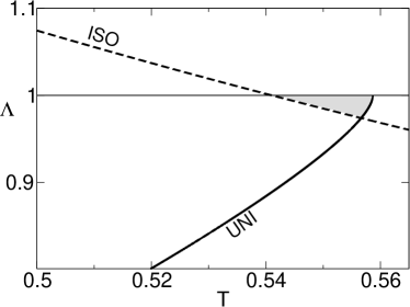
Figure 2: Temperature dependence of the eigenvalues associated with the analysis of linear stability of the fixed points of the simple MSZ model on a Cayley tree of coordination $q=3$. The grey region indicates the joint range of stability ($|\Lambda_{\mathrm{iso}}|<1$ and $|\Lambda_{\mathrm{uni}}|<1$).

We now resort to a special technique Gujrati ; Stilck to find the free energy associated with the bulk attractors of the recursion relations. The idea of the method is to calculate that free energy by cleverly subtracting the contribution from the surface sites. According to an argument of Gujrati Gujrati , we first write the free energy of a Cayley tree with $M$ layers,

$$F_{M} = -\frac{1}{\beta}\ln\mathcal{Z}_{M}$$ (22)

$$= f_{0}^{(M)}+qf_{1}^{(M)}+q(q-1)f_{2}^{(M)}+\cdots$$

$$+q(q-1)^{M-1}f_{M-1}^{(M)},$$

where $\mathcal{Z}_{M}$ is the total partition function, defined in Eq. (4), and $f_{j}^{(M)}$ is the free energy per site of molecules located at the $j$th layer of the tree, while the coefficients of the $f_{j}^{(M)}$ are the number of sites in the $j$th layer. We now rewrite this last equation as

$$F_{M}=f_{0}^{(M)}+q\sum_{j=1}^{M}\left(q-1\right)^{j-1}f_{j}^{(M)},$$

and notice that for a tree with $M-1$ layers we can write

$$\left(q-1\right)F_{M-1}=\left(q-1\right)f_{0}^{(M-1)}+q\sum_{j=1}^{M-1}\left(q-1\right)^{j}f_{j}^{(M-1)}.$$

(The factor $q-1$ enters due to the fact that a $M$-layer tree has as many surfaces sites as $q-1$ trees with $M-1$ layers each.) As $M\rightarrow\infty$, the free energies per site at the surface of both trees, $f_{M}^{(M)}$ and $f_{M-1}^{(M-1)}$, should become identical. In fact, we expect that $f_{j}^{(M)}-f_{j-1}^{(M-1)}\rightarrow 0$ for all values of $j$. Thus,

$$F_{M}-\left(q-1\right)F_{M-1}\rightarrow f_{0}^{(M)}+f_{0}^{(M-1)}.$$ (23)

Since $f_{0}^{(M)}$ is the free energy associated with the central site of a $M$-layer tree, and the properties of this central site, for large $M$, are governed by the fixed points of Eqs. (16) and (17), we should have

$$\lim_{M\rightarrow\infty}f_{0}^{(M)}=\lim_{M\rightarrow\infty}f_{0}^{(M-1)}\equiv f_{b},$$

the free energy per site $f_{b}$ thus representing all sites in the Bethe lattice. Therefore, we conclude from Eqs. (22) and (23) that

$$f_{b}=-\frac{1}{2\beta}\lim_{M\rightarrow\infty}\ln\frac{\mathcal{Z}_{M}}{\left(\mathcal{Z}_{M-1}\right)^{q-1}}.$$

We then use Eqs. (4) and (10)-(15) in the limit $M\rightarrow\infty$ to write the free energy

$$f_{b}\equiv f_{b}(q,A/T;S,\eta),$$ (24)

where $S$ and $\eta$ are obtained from the fixed-point values of $\rho^{x}$ and $\rho^{y}$ via Eqs. (18) and (19), and then determine which solution corresponds to thermodynamic equilibrium. In Figure 3, we show a graph of the uniaxial order parameter, $S$, in terms of temperature. The dashed line corresponds to a coexistence of ordered ($S\neq 0$) and disordered ($S=0$) solutions.

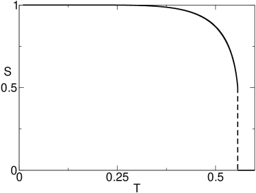
Figure 3: Graph of the order parameter $S$ versus temperature ($1/T=\beta Aq$) for the MSZ model on a Bethe lattice of coordination $q=3$. The dashed vertical line indicates a first-order transition.

III Lattice model for a binary mixture of rods and disks

Given a configuration $\left\{\lambda_{i}\right\}$ of rodlike ($\lambda_{i}=+1$) and disklike ($\lambda_{i}=-1$) molecular aggregates, the energy of the MSZ model for a binary mixture is written as

$$\mathcal{H}\left\{\lambda_{i}\right\}=-A\sum_{(i,j)}\sum_{\mu\nu=x,y,z}\lambda_{i}S_{i}^{\mu\nu}\lambda_{j}S_{j}^{\mu\nu},$$ (25)

which leads to the canonical partition function

$$Z_{B}={\displaystyle\sum_{\left\{\lambda_{i}\right\}}}^{\prime}\sum_{\left\{\overrightarrow{n}_{i}\right\}}\exp\left[\beta A\sum_{(i,j)}\sum_{\mu,\nu=x,y,z}\lambda_{i}\lambda_{j}S_{i}^{\mu\nu}S_{j}^{\mu\nu}\right].$$ (26)

The sum over $\left\{\lambda_{i}\right\}$ is restricted by the fixed concentrations of the molecular types,

$$N_{r}-N_{d}=\sum_{i=1}^{N}\lambda_{i},\quad N_{d}=N-N_{r},$$ (27)

where $N_{r}$ ($N_{d}$) is the number of rodlike (disklike) molecules, and $N$ is the total number of molecules. It is now convenient to introduce a chemical potential and change to a grand-canonical ensemble,

$$\Xi_{B}={\displaystyle\sum\limits_{N_{r}=0}^{N}}\exp\left(\beta\mu N_{r}\right)Z_{B}={\displaystyle\sum\limits_{\left\{\lambda_{i}\right\}}}\sum_{\left\{\overrightarrow{n}_{i}\right\}}\exp\left[-\beta\mathcal{H}_{\mathrm{eff}}\right],$$ (28)

with unrestricted sums over the sets of variables, and the effective Hamiltonian

$$\mathcal{H}_{\mathrm{eff}}=-\frac{\mu}{2}\left(\sum_{i=1}^{N}\lambda_{i}+N\right)-A\sum_{(i,j)}\sum_{\mu,\nu=x,y,z}\lambda_{i}\lambda_{j}S_{i}^{\mu\nu}S_{j}^{\mu\nu}.$$ (29)

Figure 4: Two examples of configurations of rods and disks on the sites of a Cayley tree of coordination $q=3$.

Along the lines of the treatment of Section 2 for the simple MSZ model on a Cayley tree, we introduce some extra states to account for rod and disk variables ($\lambda_{i}=\pm 1$), and define a set of six partial grand-canonical partition functions, $\Xi_{n}^{r,x}$, $\Xi_{n}^{r,y}$, $\Xi_{n}^{r,z}$, $\Xi_{n}^{d,x}$, $\Xi_{n}^{d,y}$, $\Xi_{n}^{d,z}$, associated with a tree of coordination $q$ with $n$ surrounding layers (see Figure 4). The notation is such that $\Xi_{n}^{r,z}$ represents the partial grand-canonical partition function of the tree with the central site in a state with $\lambda_{i}=+1$ (rodlike) and $\vec{n}_{i}$ along the $z$ direction, $\vec{n}_{i}=\pm(0,0,1)$. In analogy to equations (10) to (12), it is straightforward to write

$$\Xi_{n}^{r,x}=e^{\beta\mu}\left[e^{\frac{3\beta A}{2}}\mathcal{Q}_{n}^{r,x}+e^{\frac{-3\beta A}{4}}(\mathcal{Q}_{n}^{r,y}+\mathcal{Q}_{n}^{r,z})+e^{\frac{-3\beta A}{2}}\mathcal{Q}_{n}^{d,x}+e^{\frac{3\beta A}{4}}(\mathcal{Q}_{n}^{d,y}+\mathcal{Q}_{n}^{d,z})\right]^{q},$$ (30)

$$\Xi_{n}^{r,y}=e^{\beta\mu}\left[e^{\frac{3\beta A}{2}}\mathcal{Q}_{n}^{r,y}+e^{-\frac{3\beta A}{4}}(\mathcal{Q}_{n}^{r,z}+\mathcal{Q}_{n}^{r,x})+e^{\frac{-3\beta A}{2}}\mathcal{Q}_{n}^{d,y}+e^{\frac{3\beta A}{4}}(\mathcal{Q}_{n}^{d,z}+\mathcal{Q}_{n}^{d,x})\right]^{q},$$ (31)

$$\Xi_{n}^{r,z}=e^{\beta\mu}\left[e^{\frac{3\beta A}{2}}\mathcal{Q}_{n}^{r,z}+e^{-\frac{3\beta A}{4}}(\mathcal{Q}_{n}^{r,x}+\mathcal{Q}_{n}^{r,y})+e^{-\frac{3\beta A}{2}}\mathcal{Q}_{n}^{d,z}+e^{\frac{3\beta A}{4}}(\mathcal{Q}_{n}^{d,x}+\mathcal{Q}_{n}^{d,y})\right]^{q},$$ (32)

$$\Xi_{n}^{d,x}=\left[e^{\frac{3\beta A}{2}}\mathcal{Q}_{n}^{d,x}+e^{\frac{-3\beta A}{4}}(\mathcal{Q}_{n}^{d,y}+\mathcal{Q}_{n}^{d,z})+e^{\frac{-3\beta A}{2}}\mathcal{Q}_{n}^{r,x}+e^{\frac{3\beta A}{4}}(\mathcal{Q}_{n}^{r,y}+\mathcal{Q}_{n}^{r,z})\right]^{q},$$ (33)

$$\Xi_{n}^{d,y}=\left[e^{\frac{3\beta A}{2}}\mathcal{Q}_{n}^{d,y}+e^{\frac{-3\beta A}{4}}(\mathcal{Q}_{n}^{d,z}+\mathcal{Q}_{n}^{d,x})+e^{\frac{-3\beta A}{2}}\mathcal{Q}_{n}^{r,y})+e^{\frac{3\beta A}{4}}(\mathcal{Q}_{n}^{r,z}+\mathcal{Q}_{n}^{r,x})\right]^{q},$$ (34)

$$\Xi_{n}^{d,z}=\left[e^{\frac{3\beta A}{2}}\mathcal{Q}_{n}^{d,z}+e^{\frac{-3\beta A}{4}}(\mathcal{Q}_{n}^{d,x}+\mathcal{Q}_{n}^{d,y})+e^{\frac{-3\beta A}{2}}\mathcal{Q}_{n}^{r,z}+e^{\frac{3\beta A}{4}}(\mathcal{Q}_{n}^{r,x}+\mathcal{Q}_{n}^{r,y})\right]^{q},$$ (35)

the quantities like $\mathcal{Q}_{n}^{d,x}$ now representing partial grand-canonical partition functions of a branch with $n$ layers under the condition that the site in the innermost layer is occupied by a disk whose symmetry axis lies along the $x$ axis. The full partition function of the tree is written as

$$\Xi_{n}=\Xi_{n}^{r,x}+\Xi_{n}^{r,y}+\Xi_{n}^{r,z}+\Xi_{n}^{d,x}+\Xi_{n}^{d,y}+\Xi_{n}^{d,z}.$$ (36)

We now use a similar parametrization as in Section 2. The tensor order parameter is given by

$$Q^{\mu\nu} = \left\langle\frac{1}{N}\sum_{i}\lambda_{i}S_{i}^{\mu\nu}\right\rangle,$$ (37)

$$= \frac{3}{2}\left\langle\frac{1}{N}\sum_{i}\lambda_{i}n_{i}^{\mu}n_{i}^{\nu}\right\rangle-\frac{1}{2}\delta_{\mu\nu}\left\langle\frac{1}{N}\sum_{i}\lambda_{i}\right\rangle$$

where $\left\langle\cdots\right\rangle$ indicates a grand-canonical thermal average. The factor $\left\langle\left(\sum_{i}\lambda_{i}\right)/N\right\rangle$ gives the difference between the concentrations (number fractions) of rods and disks. It is then natural to introduce the correspondence

$$\left\langle\frac{1}{N}\sum_{i}\lambda_{i}\right\rangle\rightarrow\lim_{n\rightarrow\infty}\frac{1}{\Xi_{n}}\sum_{\nu=x,y,z}\left[\Xi_{n}^{r,\nu}-\Xi_{n}^{d,\nu}\right].$$ (38)

The ratio $\Xi_{n}^{r,z}/\Xi_{n}$ gives the concentration of rodlike particles with the symmetry axis along the $z$ direction. Terms of the form $\left(\sum_{i}\lambda_{i}(n_{i}^{\mu})^{2}\right)/N$ are recognized as the difference between the concentrations of rods and disks along the same $\mu$ direction, so that we have

$$\left\langle\frac{1}{N}\sum_{i}\lambda_{i}(n_{i}^{\mu})^{2}\right\rangle\rightarrow\lim_{n\rightarrow\infty}\frac{\Xi_{n}^{r,\mu}-\Xi_{n}^{d,\mu}}{\Xi_{n}}.$$ (39)

As in Section 2, it is interesting to work with the tensor order parameter associated with the central site of a $n$-layer tree,

$$Q_{n}^{\mu\mu}=-\frac{1}{2\Xi_{n}}\sum_{\nu}(\Xi_{n}^{r,\nu}-\Xi_{n}^{d,\nu})+\frac{3}{2}\frac{\Xi_{n}^{r,\mu}-\Xi_{n}^{d,\mu}}{\Xi_{n}},$$ (40)

such that

$$\sum_{\mu}Q_{n}^{\mu\mu}=0.$$ (41)

Again, it is convenient to introduce parameters $S_{n}$ and $\eta_{n}$ to characterize the distinct phases.

We can now write recursion relations for the branch partial partition functions $\mathcal{Q}_{n}^{\alpha,\nu}$ [formally obtained from Eqs. (30)-(35) by taking $\Xi_{n}^{\alpha,\nu}\rightarrow\mathcal{Q}_{n}^{\alpha,\nu}$, $\mathcal{Q}_{n}^{\alpha,\nu}\rightarrow\mathcal{Q}_{n-1}^{\alpha,\nu}$, and $q\rightarrow q-1$], and rewrite them in terms of the set of five ratios

$$\rho_{n}^{r,x}=\frac{\mathcal{Q}_{n}^{r,x}}{\mathcal{Q}_{n}^{r,z}},\quad\rho_{n}^{r,y}=\frac{\mathcal{Q}_{n}^{r,y}}{\mathcal{Q}_{n}^{r,z}},$$

$$\rho_{n}^{d,x}=\frac{\mathcal{Q}_{n}^{d,x}}{\mathcal{Q}_{n}^{r,z}},\quad\rho_{n}^{d,y}=\frac{\mathcal{Q}_{n}^{d,y}}{\mathcal{Q}_{n}^{r,z}},\quad\rho_{n}^{d,z}=\frac{\mathcal{Q}_{n}^{d,z}}{\mathcal{Q}_{n}^{r,z}},$$

whose connection to the physical parameters $S_{n}$ and $\eta_{n}$ is easily determined from Eqs. (30)-(35). The resulting five-dimensional nonlinear mapping problem can be investigated as in the previous section. The linear-stability analysis of the fixed points is then reduced to studying the eigenvalues of a $5\times 5$ matrix, analogous to that defined in Eq. (20).

Depending on the values of temperature and chemical potential, there appears a biaxial nematic fixed point ($S\neq 0$ and $\eta\neq 0$) besides two distinct uniaxial nematic fixed points (with $S\neq 0$ and $\eta=0$); of course, there is also an isotropic fixed point ($S=0$ and $\eta=0$). In the $\mu\times T$ plane (see Fig. 5), there is a large low-temperature region of stability of both uniaxial fixed points. However, the fixed point associated with the biaxial nematic structure is dynamically unstable.

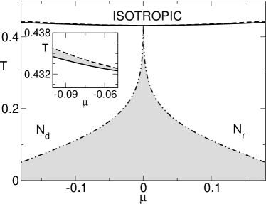
Figure 5: Stability lines in the $\mu\times T$ plane for a mixture of rodlike and disklike molecules on a Cayley tree with coordination $q=3$. Above the continuous line the isotropic phase is dynamically stable; below the dashed line at least one of the nematic uniaxial phases is dynamically stable; and between the dotted-dashed lines the two nematic uniaxial phases are dynamically stable. The biaxial nematic phase is dynamically unstable.

The existence of common regions of stability of distinct fixed points requires the analysis of the associated free energy in order to sort out the physically acceptable phases and to locate the coexistence (first-order) boundaries. Again, we use Gujrati’s method to deal with the subtleties of a Cayley tree. As in Section 2, the free energy is written in terms of the function

$$f_{b}^{\mathrm{mix}}\equiv f_{b}^{\mathrm{mix}}(q,A/T,\mu;\rho^{r,x},\rho^{r,y},\rho^{d,x},\rho^{d,y},\rho^{d,z}).$$ (42)

The phase diagram for a tree of a typical coordination, $q=3$, is shown in Figure 6. At high temperatures, there is an isotropic phase ($S=\eta=0$). At low temperatures, there are two distinct uniaxial nematic phases, $N_{r}$, with $S>0$ and $\eta=0$, with an excess of rods, and $N_{d}$, with $S<0$ and $\eta=0$, with an excess of disklike particles. In this thermalized formulation of the MSZ model, besides the biaxial nematic fixed point be dynamically unstable, it is associated with larger values of the free energy as compared to the uniaxial solutions, and cannot be thermodynamically acceptable for all coordinations $q\geq 3$. Of course, in the limit of infinite coordination ($q\rightarrow\infty$, $A\rightarrow 0$, with $qA$ fixed), we recover all of the well-known results of the mean-field calculations. Finally, in Figure 7 we show the dynamic-stability lines of the isotropic and of the uniaxial nematic phases. As expected, the first-order transition line lies between the two stability lines.

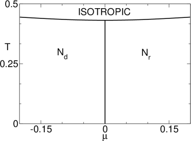
Figure 6: Phase diagram of the MSZ model for a mixture of rods and disks on the Bethe lattice (of coordination $q=3$). We indicate two uniaxial nematic ($N_{r}$ and $N_{d}$) and an isotropic phase, which are bordered by first-order transition lines.

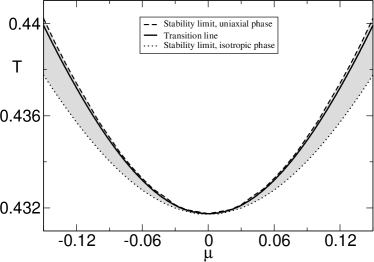
Figure 7: Phase diagram presenting the nematic-isotropic first-order transition line and the two lines which indicate the dynamic-stability limit of these two phases. As expected the transition line lies in the region (shown in grey) where there is an overlap of dynamically stability of the isotropic and the uniaxial nematic phases.

From the experimental point of view, it is interesting to draw the corresponding temperature-concentration phase diagram. We note that $c=-\partial f_{b}/\partial\mu$, and perform a Legendre transformation to eliminate the chemical potential. In Figure 8, we draw the characteristic tie lines between coexisting uniaxial nematic phases. The regions of coexistence of isotropic and nematic phases are too narrow to be clearly represented in this phase diagram.

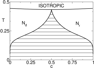
Figure 8: Temperature-concentration phase diagram of the MSZ model for a mixture of rods and disks on a Bethe lattice of coordination $q=3$. The tie lines indicate the coexistence of the uniaxial nematic phases, $N_{r}$ (rodlike molecules rich) and $N_{d}$ (disklike molecules rich). There is no stable biaxial nematic phase.

IV Conclusions and perspectives

We have formulated the problem of a Maier-Saupe-Zwanzig model on a Cayley tree as a set of nonlinear discrete recursion relations, whose attractors correspond to physically acceptable solutions on the Bethe lattice (deep in the interior of the tree). Due to the presence of first-order transitions, we have large regions of overlap of stability of distinct attractors. We then resort to an ingenious scheme to obtain the Bethe-lattice free energy associated with the coexisting attractors and to determine the thermodynamically acceptable solutions.

We first considered the simple MSZ model on a Cayley tree. In this problem, there are just two fixed points, corresponding to disordered and uniaxial ordered structures, which are both (dynamically) stable in a certain intermediate range of temperatures, and which is an indication of occurrence of a first-order transition. We then use Gujrati’s method to locate the first-order boundary between the high temperature isotropic and the low temperature uniaxial nematic phases. The MSZ model for a binary mixture comes from the introduction of a new set of shape variables and the definition of an effective Hamiltonian in the grand-canonical ensemble. The problem is more involved, but we can perform a relatively simple stability analysis of the fixed points, and draw a phase diagram in terms of temperature and chemical potential. At low temperatures, we find large regions of overlap of stability of fixed points associated with uniaxial phases. However the biaxial structure is unstable both from a dynamic-stability and a thermodynamic standpoint. The main qualitative features of the phase diagrams on the Bethe lattice agree with previous mean-field predictions Docarmo .

The framework employed in the study of the binary mixture can be extended in straightforward ways to deal with more complicated interaction potentials, although of course requiring greater analytical effort. An obvious extension is to consider a pair interaction described by

$$\sum_{\mu,\nu}\left[\lambda_{i}\lambda_{j}+b\left(\lambda_{i}+\lambda_{j}\right)+c\right]S_{i}^{\mu\nu}S_{j}^{\mu\nu},$$

which breaks the symmetry between rod-rod and disk-disk interactions. It is also possible to introduce dilution and isotropic repulsive forces to mimic the interaction potentials leading to stable biaxial phases in recent computer simulations key-4 . We hope to report on such extensions in future publications. Other extensions possibly leading to stabilization of a biaxial phase in mixtures, such as the introduction of polidispersity key-5 ; key-6 , can also be considered, at least in principle, although the analytical work becomes quite involved.

- (1) B. R. Acharya et al., Pramana 61, 231 (2003); B. R. Acharya, A. Primak, and S. Kumar, Phys. Rev. Lett. 92, 145506 (2004); L. A. Madsen, T. J. Dingemans, M. Nakata, and E. T. Samulski, Phys. Rev. Lett. 92, 145505 (2004); K. Merkel et al., Phys. Rev. Lett. 93, 237801 (2004).
- (2) See e.g. R. Berardi et al., J. Phys.: Condens. Matter 20, 463101 (2008).
- (3) D. Apreutesei and G. H. Mehl, Chem. Commun. 2006, 609 (2006).
- (4) A. Cuetos, A. Galindo, and G. Jackson, Phys. Rev. Lett. 101, 237802 (2008).
- (5) P. Palffy-Muhoray, J. R. de Bruyn, and D. A. Dunmur, Mol. Cryst. Liq. Cryst. 127, 301 (1985), and J. Chem. Phys. 82, 5294 (1985); S. R. Sharma, P. Palffy-Muhoray, B. Bergersen, and D. A. Dunmur, Phys. Rev. A 32, 3752 (1985).
- (6) E. F. Henriques and V. B. Henriques, J. Chem. Phys. 107, 8036 (1997); E. F. Henriques, C. B. Passos, V. B. Henriques, and L. Q. Amaral, Liquid Crystals 35, 555 (2008).
- (7) L. J. Yu and A. Saupe, Phys. Rev. Lett. 45, 1000 (1980); Y. Galerne and J. P. Marcerou, Phys. Rev. Lett. 51, 2109 (1983); A. A. de Melo-Filho, A. Laverde, and F. Y. Fujiwara, Langmuir 19, 1127 (2003).
- (8) E. do Carmo, D. B. Liarte, and S. R. Salinas, Phys. Rev. E 81, 062701 (2010).
- (9) R. J. Baxter, Exactly solved models in statistical mechanics, Academic Press, New York, 1982.
- (10) C. J. Thompson, J. Stat. Phys. z 27, 441 (1982).
- (11) P. D. Gujrati, Phys. Rev. Lett. 74, 809 (1995).
- (12) T. P. Eggarter, Phys. Rev. B 9, 2989 (1974).
- (13) M. J. de Oliveira, A. M. Figueiredo Neto, Phys. Rev. A 34, 3481 (1986).
- (14) P. G. de Gennes and J. Prost, The Physics of Liquid Crystals, Oxford University Press, Oxford, 1995.
- (15) M. J. de Oliveira and S. R. Salinas, Rev. Bras. Fis. 15, 189 (1985).
- (16) T. J. Oliveira, J. F. Stilck and P. Serra, Phys. Rev. E 80, 041804 (2009).
- (17) Y. Martínez-Ratón and J. A. Cuesta, Phys. Rev. Lett. 89, 185701 (2002).
- (18) L. Longa, G. Pająk, and T. Wydro, Phys. Rev. E 76, 011703 (2007).