IPMU10-0140

Cascade supersymmetry breaking
and
low-scale gauge mediation
Masahiro Ibe¹, Yuri Shirman¹ and Tsutomu T. Yanagida²

¹ Department of Physics & Astronomy, University of California, Irvine, CA 92697, USA
² Institute for the Physics and Mathematics of the Universe, University of Tokyo,
Kashiwa 277-8568, Japan

1 Introduction

The gauge mediated supersymmetry breaking (GMSB) models [1, 2, 3, 4, 5, 6, 7] provide one of the most attractive realizations of the phenomenologically acceptable minimal supersymmetric standard model (MSSM). The gravitino is the lightest supersymmetric particle whose mass ranges from the eV to the GeV. This feature of gauge mediation motivated a lot of theoretical works on phenomenological and cosmological aspects of the models [8].

Light gravitino models are constrained by cosmological and astrophysical problems. In particular, the analysis of CMB data and the Lyman-$\alpha$ forest data put an upper bound of 16 eV on the gravitino mass [9]. Furthermore, future cosmic microwave background observations will probe gravitino mass down to the eV range [10]. Thus, models with very light gravitino are particularly interesting. Such models require a very low fundamental scale of supersymmetry (SUSY) breaking and as a result may have very rich collider phenomenology.

Models with such a light gravitino (see for example Ref.[11, 12, 13, 14, 15]) generically suffer from a range of theoretical problems: the Standard Model couplings hit the Landau pole below the scale of the Grand Unification Theory (GUT); gaugino masses are suppressed compared to the sfermion masses; there are supersymmetric ground states in the vicinity of desired SUSY breaking vacua. Much of the parameter space in this class of models has been excluded by the neutralino/chargino mass limit [16, 24, 18] at the Tevatron experiments [19] or by the vacuum stability problem [20] for the gravitino lighter than $16$ eV. In this paper, we propose a new class of the GMSB models, the cascade supersymmetry breaking, which may avoid these problems.

The organization of the paper is as follows. In section 2, we briefly review problems arising in attempts to construct low scale GMSB models. In section 3, we introduce a generic idea of the cascade supersymmetry breaking. An example based on dynamical supersymmetry breaking (DSB) is introduced in section  4. In sections  5, we study phenomenological features of the model, messenger and superpartner spectra as well as possible generalizations. In section 6, we comment on a relation of our model to the conformal gauge mediation mechanism developed in Ref.[21]. The final section is devoted to the conclusions and some discussions.

2 A brief review of low scale gauge mediation

2.1 Scales in light gravitino scenario

Since we are interested in models with the gravitino mass in the eV range, the fundamental SUSY breaking scale must be low,

$$\sqrt{F}\sim 65\,{\rm TeV}\times\left(\frac{m_{3/2}}{1\,{\rm eV}}\right)^{1/2}\ .$$ (1)

Such a low SUSY breaking scale can be achieved in GMSB models. Indeed, in the simplest GMSB models, the superpartner masses are given by

$$\tilde{m}\sim\frac{\alpha}{4\pi}\frac{F_{S}}{m}\,,$$ (2)

where $m$ is the messenger scale and $F_{S}$ is a mass splitting within messenger multiplets. One must also require $F_{S}<m^{2}$ to avoid tachyonic messengers and charge-color breaking. Thus, a requirement that the superpartners have mass at the electroweak scale leads to the lower bound on the mass parameters in the messenger sector,

$$m\sim\sqrt{F_{S}}\sim O(10-100)\,{\rm TeV}\ .$$ (3)

We see that light gravitino scenarios can only be realized when the SUSY breaking effects in the messenger sector are comparable to the fundamental scale of SUSY breaking, $F_{S}\sim F$. To avoid the separation of scales, one must look at models of direct or semi-direct gauge mediation. Furthermore, one expects that successful models will necessarily be strongly coupled.

2.2 R-symmetry and the messenger sector

Let us briefly review difficulties encountered in search for models of low scale gauge mediation. We begin by considering a simple example of the messenger sector:

$$W=\Lambda_{1}^{2}S+(m_{ij}+\lambda_{ij}S)\bar{\psi}_{i}\psi_{j}\ ,$$ (4)

Where $S$ is a supersymmetry breaking field and $\psi$, $\bar{\psi}$ are messenger fields. This model possesses an R-symmetry (under which $S$ has charge 2) if the charges of the messenger fields can be chosen such that [22, 23]:

$$m_{ij}\neq 0~{}\Rightarrow~{}R(\psi_{i})+R(\psi_{j})=2;\hskip 36.135pt\lambda_{ij}\neq 0~{}\Rightarrow~{}R(\psi_{i})+R(\psi_{j})=0\,.$$ (5)

We will restrict our attention to models with $\det m\neq 0$. Indeed, models with $\det m=0$ are problematic from phenomenological perspective because the true vacuum in this case is a charge-color breaking one (for detailed analysis of the vacuum structure of this class of models see Ref.[23]). When parameters are chosen so that the gravitino mass is in the $\mathcal{O}(10\,\mathrm{eV})$ range, the charge-color breaking ground states are found in the vicinity of the charge-color preserving minima of the potential. This leads to two problems with the desired minimum: first, the lifetime of this minimum is expected to be too short; second, initial conditions must be fine-tuned for it to be selected in the course of cosmological evolution.

Furthermore, the lifetime of the vacuum in the models with light gravitino and supersymmetric runaway directions is too short. We will, therefore, require that $\lambda m^{-1}\lambda=0$ which guarantees the absence of the runaway directions [24]. With these assumptions, the model in Eq.(4) possesses the following important features

• The supersymmetry is broken;

• The effective mass matrix for messenger fields is independent of the vacuum expectation value (vev) of the pseudo-modulus:

  $$\det(m_{ij}+\lambda_{ij}S)=\det m_{ij}\neq 0\ .$$ (6)

A phenomenologically viable model requires that the R-symmetry is broken (otherwise the Standard Model gauginos remain massless). This can be achieved through introduction of additional fields and interactions that lead to either spontaneous or explicit R-symmetry breaking. However, this is often insufficient. Indeed, as long as the effective messenger mass matrix satisfies Eq.(6), the gaugino masses vanish at the leading order in $F_{S}$ [27]

$$m_{\tilde{g}}=\left.\frac{\alpha}{4\pi}\log\left[\det(m_{ij}+\lambda_{ij}S)\right]\right|_{\rm\theta^{2}}=0\ .$$ (7)

The first contribution to gaugino masses appears only at the order $F_{S}^{3}$ [11],

$$m_{\rm gaugino}\sim c\frac{\alpha}{4\pi}\frac{F_{S}}{m}\left|\frac{F_{S}}{m^{2}}\right|^{2}\ .$$ (8)

The sfermion masses are still generated at the leading order in $F_{S}$ and the requirement that gaugino and sfermion masses are comparable can only be satisfied in models of low scale SUSY breaking. However, it turns out that the coefficient $c$ is small and sufficiently large gaugino masses can not be achieved without fine-tuning. Furthermore, detailed numerical analysis, has shown that, even with $c=O(1)$, the predicted gaugino masses have been almost excluded by Tevatron constraints on the neutralino/chargino masses for $m_{3/2}\lesssim 16$ eV [16, 24, 18].

Thus, we must turn to models where Eq.(5) is not satisfied in the messenger sector. In such models, gaugino masses are unsuppressed, however, the SUSY breaking vacuum is only a local one. To see this, note that at least at one point along the pseudo-flat direction the matrix $m_{ij}+\lambda_{ij}S$ has a zero eigenvalue and at least one pair of messengers becomes massless. They can now acquire vevs and restore supersymmetry. To ensure sufficiently long vacuum lifetime, one must increase the messenger mass $m$. This suppresses all superpartner masses if the gravitino mass (and, therefore, the fundamental scale of SUSY breaking) is kept fixed. In particular, for $m_{3/2}\lesssim 16$ eV, the detailed numerical analysis  [20] has lead to an upper bound on superpartner masses of about $1$ TeV.

2.3 Direct and semi-direct gauge mediation

A toy model discussed above implied direct or semi-direct gauge mediation. Additional problems often arise when UV complete realizations of direct gauge mediation is considered (a precise definition of direct gauge mediation is given in [28, 29] while semi-direct gauge mediation is introduced in [31]). The messengers play a dual role in direct GMSB models — in addition to communicating the supersymmetry breaking to the Standard Model fields, they play a role in SUSY breaking dynamics. The need for a large flavor symmetry in the DSB sector usually implies that the DSB gauge group is large itself. As a result, the Standard Model gauge interactions have Landau poles below the GUT scale when the messenger scale is low. If one insists on perturbative coupling unification, both the messenger and SUSY breaking scales are pushed up preventing the possibility of light gravitino. This latter difficulty may be avoided in semi-direct gauge mediation [21, 31] (see also Refs.[32, 33] for earlier attempts), where messengers are charged under the DSB group but do not play a direct role in SUSY breaking. This allows to construct models with small number of messengers and avoid Landau pole problems. However, the leading contribution to the gaugino mass is again vanishing due to the R-symmetry (see also Ref.[34]).

3 Cascade supersymmetry breaking

In order to solve problems discussed in the previous section we will employ some of the tools proposed in the original GMSB models[5, 6, 7] – namely we will introduce a secondary SUSY breaking sector. Despite the existence of several sectors, our model will have all the desirable features of direct (and semi-direct) gauge mediation. Finally, in a strong coupling limit, we will be able to obtain low SUSY breaking scale. We will refer to this class of models as cascade SUSY breaking .

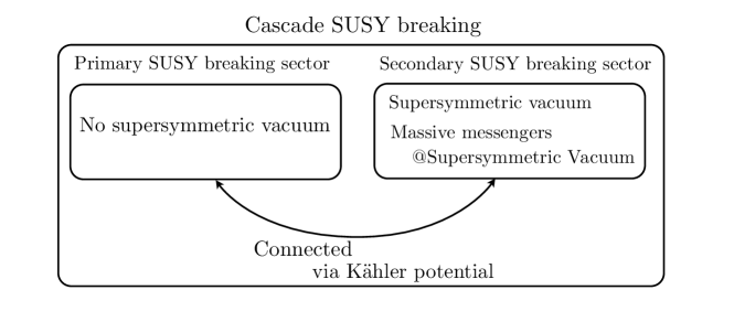
Figure 1: A schematic picture of the cascade supersymmetry breaking. Supersymmetry breaking in the secondary sector is induced by the primary supersymmetry breaking via the connections in the Kähler potential.

To illustrate the idea of cascade gauge mediation, we consider a model with the following superpotential

$$W = \Lambda_{1}^{2}S+\Lambda_{2}^{2}X-\frac{f}{3}X^{3}+kX\bar{\psi}\psi\ .$$ (9)

Here, $S$ represents a field of the primary SUSY breaking sector, while $X$, $\psi$, and $\bar{\psi}$ are fields in the secondary sector (with latter two serving as messengers). We have assumed that the superpotential couplings between the two sectors are suppressed. In section 4 we will introduce a dynamical model with absence of the superpotential interactions between the two sectors will be ensured by symmetries. The two sectors will interact only through the Kähler potential  (see Fig. 1):

$$K = |S|^{2}+|X|^{2}+\frac{c_{SP}}{\Lambda^{2}}|S|^{2}|X|^{2}+\cdots\ ,$$ (10)

In the decoupling limit, $c_{SP}=0$, SUSY is broken in the primary sector, while the secondary sector possesses a supersymmetric minimum with spontaneously broken R-symmetry :

$$F_{S}=\Lambda_{1}\,,~{}~{}~{}X={\Lambda_{2}}/{f^{1/2}}\,,~{}~{}~{}\langle\bar{\psi}\psi\rangle=0\,.$$ (11)

Once the coupling between two sectors is turned on, $c_{SP}\neq 0$, supersymmetry breaking in the primary sector induces supersymmetry breaking in the secondary sector through higher dimensional operators. Indeed $X$ potential becomes

$$V=-m_{\rm soft}^{2}|X|^{2}+|\Lambda_{2}^{2}+fX^{2}|^{2}\ ,$$ (12)

where

$$m_{\rm soft}^{2}=c_{SP}\frac{|F_{S}|^{2}}{\Lambda_{1}^{2}}\ .$$ (13)

We see that $X$ obtains a non-vanishing $F$-term vev which, in the limit $|m_{\rm soft}|\ll\Lambda_{2}$, is given by

$$F_{X}=\frac{m_{\rm soft}^{2}}{2f}\ .$$ (14)

Now SUSY breaking effects are mediated to the MSSM sector due to the coupling $kX\bar{\psi}\psi$. One finds a standard expression for gaugino masses

$$m_{\tilde{g}}\sim\frac{\alpha}{4\pi}\log X|_{\theta^{2}}\neq 0\ .$$ (15)

The very light gravitino is realized when all the dimensioneless coefficients are of order one while the mass scales in the Lagrangian are comparable, i.e.,

$$\sqrt{F}_{S}\sim\Lambda_{\rm 2}\sim\Lambda_{1}\sim m\ .$$ (16)

In this limit, the supersymmetry breaking and the messenger mass scales are of the same order of magnitude,

$$F_{X}\sim F_{S}\ ,\quad\left\langle{X}\right\rangle\sim\sqrt{F_{X}}\sim\Lambda_{1,2}\ ,$$ (17)

as required to obtain light gravitino.

Before closing this section, we comment on the sign of $c_{SP}$. The SUSY breaking effects discussed above shift the $X$ vev independently of the sign of $c_{SP}$. The model may be further simplified when $c_{SP}$ is positive. In this case, the following superpotential is sufficient to induce SUSY breaking effects in the secondary sector:

$$W=\frac{f}{3}X^{3}+kX\bar{\psi}\psi\ .$$ (18)

There exist a supersymmetric minimum at $\left\langle{X}\right\rangle=0$ where messengers are massless. However, if $c_{SP}>0$ the supersymmetric vacuum is “destabilized”, and both the scalar and the $F$-term components obtain non-vanishing expectation values.

4 A model of cascade supersymmetry breaking

The superpotential Eq.(9) of our toy model is not the most general one consistent with the symmetry. More importantly, the model possesses a supersymmetric charge-color breaking vacuum. The existence of this vacuum places significant constraints since it may be hard to ensure sufficiently long lifetime of the SUSY breaking vacuum. Finally, conditions Eq.(16) must be satisfied in light gravitino scenario. This implies that the model is strongly coupled and requires UV completion.

In this section, we introduce UV complete description of the cascade SUSY breaking based on the $SP(N_{c})\times SU(4)$ gauge theory with the matter contents given in Table 1. The Standard Model gauge groups will be embedded into the global $SU(5)_{\rm SM}$ symmetry. We choose tree level superpotential to be

$$W=\lambda_{ij}S_{ij}Q^{i}Q^{j}+m_{R}\bar{R}R+m_{F}\bar{F}F\ ,$$ (19)

where $\lambda$’s is a coupling constant, and $m_{R,F}$ denote mass parameters. Let us first choose parameters that will simplify the analysis of SUSY breaking:

$$m_{R}\gg\Lambda_{1},\,\Lambda_{2}\gg m_{F}\ ,$$ (20)

where $\Lambda_{1}$ and $\Lambda_{2}$ are dynamical scales of $SP(N_{c})$ and $SU(4)$ groups respectively. In this regime, we can integrate out massive $\bar{R}$ and $R$ fields and the dynamics of two gauge groups, $SP(N)$ and $SU(4)$, decouples to the leading order . Dynamical scales of the two low energy gauge groups are given by

$$\Lambda^{\prime 2(N_{c}+1)}_{1}=m_{R}^{4}\Lambda^{2(N_{c}+1)-4}_{1},~{}~{}~{}\Lambda^{\prime 7}_{2}=m_{R}^{2N_{c}}\Lambda_{2}^{7-2N_{c}}$$ (21)

Notice that the $SU(4)$ gauge group is asymptotically free above $m_{R}$ for $N_{c}<4$, while $SP(N_{c})$ group is asymptotically free for $N_{c}>1$.

Table 1: The field content of the model based on $SP(N_{c})\times SU(4)$ gauge theory. Here, we also show global symmetries of the model $SU(5)_{\rm SM}$ and $SU(2(N_{c}+1))$.

$$\begin{array}[]{|c||c|c||c|c| l}\cline{1-5}\cr&SP(N_{c})&SU(4)&SU(5)_{\rm SM}&SU(2(N_{c}+1))&\\ \cline{1-5}\cr\vskip-0.4pt\cr\vskip-0.4pt\cr\vskip-0.4pt\cr\vskip-0.4pt\cr\cline{1-5}\cr Q&\mathbf{2N_{c}}&\mathbf{1}&\mathbf{1}&\mathbf{2(N_{c}+1)}&\raisebox{-6.99997pt}[0.0pt][0.0pt]{{\Large\} } Primary Sector }\\ S_{ij}&\mathbf{1}&\mathbf{1}&\mathbf{1}&\mathbf{(N_{c}+1)(2N_{c}+1)}\\ (F,\bar{F})&(\mathbf{1},\mathbf{1})&(\mathbf{4},\mathbf{4}^{*})&(\mathbf{5},\mathbf{5}^{*})&\mathbf{1}&\hskip 14.22636pt\text{Secondary Sector}\\ (R,\bar{R})&(\mathbf{2N_{c}},\mathbf{2N_{c}})&(\mathbf{4},\mathbf{4}^{*})&\mathbf{1}&\mathbf{1}&\hskip 14.22636pt\text{Connector}\\ \cline{1-5}\cr\end{array}$$

4.1 Primary supersymmetry breaking sector

In the limit $m_{R}\rightarrow\infty$, the $SP(N_{c})$ dynamics breaks SUSY through IYIT mechanism [38] and we will refer to this sector as a primary SUSY breaking sector. Let us briefly review the dynamics of this sector. Below $m_{R}$ the physics is described by an $SP(N_{c})$ gauge group and $N_{c}+1$ flavors and a set of gauge singlet fields. The full superpotential is given by the sum of tree level terms and the quantum constraint:

$$W=\lambda_{ij}S_{ij}Q_{i}Q_{j}+{\cal X}(\mathrm{Pf}(QQ)-{\Lambda^{\prime}}_{1}^{2(N_{c}+1)})\ ,$$ (22)

where $\cal X$ is a Lagrange multiplier. This superpotential is inconsistent with the supersymmetric ground state. A convenient description of the dynamics can be obtained in terms of the meson fields $V_{ij}=Q_{i}Q_{j}$. These fields marry singlets and become massive. Thus, the low energy theory contains only a single gauge singlet field with the superpotential

$$W=\lambda\Lambda^{\prime 2}_{1}S\ ,$$ (23)

where $S={\rm Pf}(S_{ij})^{1/(N_{c}+1)}$. The Kähler potential has the form

$$K=|S|^{2}+\eta_{S}\frac{|S|^{4}}{\Lambda^{\prime 2}_{1}}\,.$$ (24)

For small $\lambda$, the coefficient $\eta_{S}$ is calculable and negative [41] ensuring that the vacuum is at the origin:

$$S = 0\ ,$$ (25)

$$F_{S} = \lambda\Lambda_{1}^{\prime 2}=\lambda m_{R}^{4/(N_{c}+1)}\Lambda_{1}^{(2(N_{c}+1)-4)/(N_{c}+1)}\ .$$ (26)

4.2 Secondary supersymmetry breaking sector

Below $m_{R}$ the secondary sector is described by an s-confining $SU(4)$ gauge theory [42],

$$W=m_{F}\mathop{\rm tr}M+\frac{\det M-\bar{B}MB}{\Lambda_{2}^{\prime 7}}=m_{F}\mathop{\rm tr}M+\frac{\det M-\bar{B}MB}{m_{R}^{2N_{c}}\Lambda_{2}^{7-2N_{c}}}\ ,$$ (27)

where

$$M_{a}^{\bar{a}} = F_{a}\bar{F}^{a}\ .$$ (28)

$$B_{a} = \epsilon_{\alpha_{1}\cdots\alpha_{4}}\epsilon_{aa_{1}\cdots a_{4}}\bar{F}^{\alpha_{1}a_{1}}\cdots\bar{F}^{\alpha_{4}a_{4}}\ ,$$ (29)

$$\bar{B}^{\bar{a}} = \epsilon^{\alpha_{1}\cdots\alpha_{4}}\epsilon^{\bar{a}a_{1}\cdots a_{4}}{F}_{\alpha_{1}a_{1}}\cdots{F}_{\alpha_{4}a_{4}}\ ,$$ (30)

and $\alpha$’s are the $SU(4)$ indices while $a$ and $b$ are $SU(5)_{\rm SM}$ indices. We further define rescaled fields, $X$, $\tilde{M}$, $\tilde{B}$ and $\tilde{\bar{B}}$ by $X=\sqrt{5/2}\,\mathrm{Tr}M/\Lambda_{2}^{\prime}$, $\tilde{M}^{a}_{b}=(M^{a}_{b}-\mathrm{Tr}M^{a}_{b}/5)/\Lambda_{2}^{\prime}$, $\tilde{B}=B/\Lambda_{2}^{\prime 3}$ and $\tilde{\bar{B}}=\bar{B}/\Lambda_{2}^{\prime 3}$.

The supersymmetric minimum of the secondary sector is located at

$$\left\langle{X}\right\rangle_{\rm SUSY} \simeq \sqrt{10}\left(\frac{m_{F}}{\Lambda^{\prime}_{2}}\right)^{1/4}\Lambda^{\prime}_{2}\ ,$$ (31)

$$\tilde{M} = 0\ ,$$ (32)

$$\tilde{B} = \tilde{\bar{B}}=0\ .$$ (33)

In this vacuum, all the fields charged under the global $SU(5)_{\rm SM}$ symmetry are massive.

For sufficiently small $m_{F}$, the secondary sector also possesses a metastable SUSY breaking vacuum [43]. Typically, models of direct gauge mediation make use of this metastable SUSY breaking vacuum. However, the maximal global symmetry of the secondary sector is spontaneously broken in non-supersymmetric minimum which, in turn, requires a gauge group larger than $SU(4)$ and generically leads to Landau poles for the Standard Model couplings below the GUT scale. We will instead use a supersymmetric vacuum of the secondary sector. The presence of $R$, $\bar{R}$ fields induces Kähler potential interactions between the primary and secondary sectors and generates non-vanishing $F_{X}$.

4.3 Interaction between the two sectors

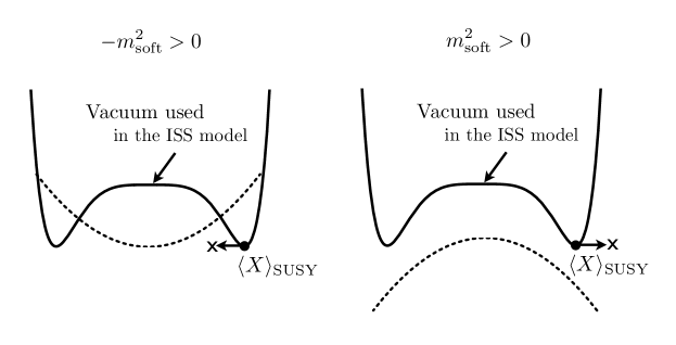
Figure 2: A schematic picture of the shift of the supersymmetric vacuum by the supersymmetry breaking mass via the Kähler potential. The solid lines show the supersymmetric scalar potential, while the dashed lines show the supersymmetry breaking potential. The vacuum used in the cascade supersymmetry breaking is denoted by “$\times$”. We have shown a local supersymmetry breaking minimum at $X=0$ discussed in Ref.[43].

After $R$, $\bar{R}$ fields are integrated out, the superpotential of the low energy theory is

$$W \simeq \lambda{\Lambda}_{1}^{\prime 2}S+\frac{5}{\sqrt{10}}\,m_{F}\Lambda_{2}^{\prime}X+\frac{1}{10^{5/2}}\frac{X^{5}}{{\Lambda}_{2}^{\prime 2}}\ ,$$ (34)

while the interactions between the two sectors are given by corrections to the Kähler potential:

$$\delta K_{1} \simeq c_{SP}\frac{|S|^{2}|X|^{2}}{m_{R}^{2}}+c_{M}\frac{|S|^{2}|\tilde{M}|^{2}}{m_{R}^{2}}+c_{B}\frac{|S|^{2}|\tilde{B}|^{2}}{m_{R}^{2}}+c_{B}\frac{|S|^{2}|\tilde{\bar{B}}|^{2}}{m_{R}^{2}}\ .$$ (35)

It is useful to note that since coupling constants in Eq.(35) are radiatively generated, they are small in the large $m_{R}$ limit. On the other hand, these couplings are of order one in a strongly coupled regime,

$$m_{R}\sim m_{F}\sim\Lambda_{1}\sim\Lambda_{2}\,.$$ (36)

A comparison of Eqs.(34) and (35) to Eqs.(9) and (10) shows that $SP(N_{c})\times SU(4)$ model represents a dynamical realization of the cascade supersymmetry breaking.

Let us analyze the spectrum of the model at weak coupling. For $|c_{SP}|\ll 1$, the $X$ vev is slightly shifted from its supersymmetric value in Eq.(31), and the size of the secondary supersymmetry breaking is expected to be much smaller than $F_{S}$ and $\Lambda_{2}^{\prime 2}$. Furthermore, the effect of the interactions on the vevs of the fields in the primary sector is negligible. Thus, the effective scalar potential of $X$ can be approximated by

$$V\simeq-m_{\rm soft}^{2}|X|^{2}+\left|-\frac{5}{\sqrt{10}}m_{F}\Lambda^{\prime}_{2}+\frac{1}{10^{5/2}}\frac{5\,X^{4}}{\Lambda_{2}^{\prime 2}}\right|^{2}\ ,$$ (37)

with

$$m_{\rm soft}^{2}={c_{SP}}\frac{|F_{S}|^{2}}{m_{R}^{2}}\ .$$ (38)

As a result, the supersymmetric vacuum in Eq.(31) is shifted to

$$\left\langle{X}\right\rangle \simeq \left\langle{X}\right\rangle_{\rm SUSY}\left(1+\frac{1}{4}\frac{m_{\rm soft}^{2}}{\sqrt{m_{F}^{3}\Lambda_{2}^{\prime}}}\right)\ ,$$ (39)

$$F_{X} \simeq \frac{10^{5/2}m_{\rm soft}^{2}\Lambda_{2}^{\prime 2}}{20\left\langle{X}\right\rangle^{2}}\simeq\left(\frac{5\Lambda_{2}^{\prime}}{2m_{F}}\right)^{1/2}m_{\rm soft}^{2}\ .$$ (40)

Here, we have assumed that $|m_{\rm soft}|$ is much smaller than $m_{F},\Lambda^{\prime}_{2}$ in the weak coupling regime.

As we have noted before the secondary supersymmetry breaking is achieved regardless of the sign of $c_{SP}$. A a schematic cartoon of the supersymmetry breaking shift in the scalar potential and its dependence on the sign of $c_{SP}$ is shown in Fig.2. The implications of the possibility of positive $c_{SP}$ are discussed in the appendix.

5 Superparnter masses

We are now ready to gauge the Standard Model subgroup of the global $SU(5)_{\rm SM}$ symmetry and consider the effects of supersymmetry breaking on the MSSM sector. We begin by studying the messenger spectrum. The $SU(4)$ gauge group confines and the composite fields, $\tilde{M}$ and ($\tilde{B}$, $\tilde{\bar{B}}$), transforming in an adjoint and fundamental representations of the $SU(5)_{\rm SM}$ will serve as messenger fields. Messengers obtain both holomorphic and D-type soft masses. The D-type soft masses arise from the Kähler potential interactions with the primary SUSY sector Eq.(35) as well as from the Kähler potential terms generated by self-interactions in the secondary sector:

$$\delta K_{2} = \eta_{M}\frac{|X|^{2}|\tilde{M}|^{2}}{\Lambda_{2}^{\prime 2}}+\eta_{B}\frac{|X|^{2}|\tilde{B}|^{2}}{\Lambda_{2}^{\prime 2}}+\eta_{B}\frac{|X|^{2}|\tilde{\bar{B}}|^{2}}{\Lambda_{2}^{\prime 2}}\ .$$ (41)

These corrections to the Kähler potential generate D-type scalar masses for messengers:

$$\left(\tilde{m}_{M}^{2}\right)_{D} = -c_{M}\frac{|F_{S}|^{2}}{m_{R}^{2}}-\eta_{M}\frac{|F_{X}|^{2}}{\Lambda_{2}^{\prime 2}}\ ,$$ (42)

$$\left(\tilde{m}_{B}^{2}\right)_{D} = -c_{B}\frac{|F_{S}|^{2}}{m_{R}^{2}}-\eta_{B}\frac{|F_{X}|^{2}}{\Lambda_{2}^{\prime 2}}\ .$$ (43)

Since $c_{M}\sim c_{B}\sim c_{\mathrm{S}P}$, these terms are of order $m_{\rm soft}^{2}$.Moreover, in the strong coupling regime, self-interactions in the secondary sector result in order 1 corrections to these masses.

In addition messengers receive holomorphic soft masses that can be obtained from Eq.(27):

$$\left(m_{M}^{2}\right)_{h} \simeq \frac{9}{10^{3/2}}\frac{\left\langle{X}\right\rangle^{2}F_{X}}{\Lambda_{2}^{\prime 2}}\,,$$ (44)

$$\left(m_{B}^{2}\right)_{h} \simeq \frac{1}{10^{1/2}}F_{X}\ .$$ (45)

Finally, supersymmetric terms in the messenger mass matrix are given by

$$m_{M} \simeq \frac{3}{10^{3/2}}\frac{\left\langle{X}\right\rangle_{\rm SUSY}^{3}}{\Lambda_{2}^{\prime 2}}\ ,$$ (46)

$$m_{B} \simeq \frac{1}{10^{1/2}}\left\langle{X}\right\rangle_{\rm SUSY}\ .$$ (47)

Note that one must choose parameters of the model in such a way that all eigenvalues of the mass squared matrix for scalar messengers are positive. This must be achieved while avoiding too large positive values of D-type soft masses squareds (otherwise gauge mediated masses for the sfermions could become negative).

With the knowledge of the messenger spectrum, we can obtain superpartner masses. To the leading order in SUSY breaking parameters, gaugino masses only depend on the holomorphic soft masses of the messenger fields [45, 46] and are given by

$$m_{\rm gaugino} \simeq -\frac{\alpha_{a}}{4\pi}\left(5\frac{\left(\tilde{m}_{M}^{2}\right)_{h}}{m_{M}}+\frac{\left(\tilde{m}_{B}^{2}\right)_{h}}{m_{B}}\right)\,.$$ (48)

A general formula describing soft sfermion masses is presented in Ref.[45]. The contribution due to non-vanishing messenger supertrace dominates the result in the large $m_{R}$ limit leading to log divergent terms

$$m_{\rm sfermion}^{2} \sim 2\left(\frac{\alpha_{a}}{4\pi}\right)^{2}C_{a}(r)m_{\rm soft}^{2}\left(5\log\frac{m_{R}^{2}}{m_{M}^{2}}+\log\frac{m_{R}^{2}}{m_{B}^{2}}\right)\ ,$$ (49)

where $C_{a}(r)$ denotes the quadratic Casimir invariant of the MSSM gauge symmetries for each sfermion of a representation $r$ and we made the use of the fact that the D-type masses are of the order $m_{\mathrm{soft}}$. Effect of the holomorphic soft messenger masses is small in the large $m_{R}$ limit,

$$m_{\rm sfermion}^{2}\sim 2\left(5+\frac{1}{9}\right)\times\left(\frac{\alpha_{a}}{4\pi}\right)^{2}C_{a}(r)\frac{(m_{M}^{2})_{h}^{2}}{m_{M}^{2}}\ .$$ (50)

To guarantee that the sfermion and gaugino masses are comparable we must take strong coupling limit Eq.(36). In this limit we can only give an estimate of superpartner masses,

$$m_{\rm gaugino} \sim \frac{\alpha_{a}}{4\pi}m_{\rm soft}\ ,$$ (51)

$$m_{\rm sfermion}^{2} \sim \left(\frac{\alpha_{a}}{4\pi}\right)^{2}m_{\rm soft}^{2}\ .$$ (52)

Nevertheless this is a desirable region of the parameter space since it results in low scale GMSB. We also note that strong coupling effects could have significant consequences for the superpartner spectrum and further suppress the hierarchy between the superpartner masses and fundamental SUSY breaking scale [47]. Since such modifications would only improve the plausibility of the light gravitino scenario, we will use the estimate (51) in the rest of the paper.

In table 2, we show a summary of scales in model that allow comparable gaugino and sfermion masses (see the appendix for the detailed analysis). In the table, we listed the appropriate mass scales for $c_{SP}<0$ and $c_{SP}>0$ separately. Notice that the sign of $c_{SP}$ is not the parameter of the model but is determined by model by model. Our case study approach just reflects our inability to calculate the sign of $c_{SP}$ due to the strong interactions.

Table 2: Summary of the model of cascade supersymmetry breaking based on $SP(N_{c})\times SU(4)$ gauge symmetries. In the parameter regions listed below, the gaugino masses and the sfermion masses are comparable. The discussions for $c_{SP}>0$ are given in the appendix. The very light gravitino is realized by taking $m_{R}$ close to $\Lambda_{2}^{\prime}$ in the cases with low scale gauge mediation (see discussion around Eq.(58)).

	mass parameters	mediation scale
$c_{SP}<0$	$\Lambda_{2}^{\prime}\sim m_{F}\sim|m_{\rm soft}|$	low scale
$c_{SP}>0$	$\Lambda_{2}^{\prime}\sim|m_{\rm soft}|$	low scale
	$m_{F}$ can be small
$c_{SP}>0$	$\Lambda_{2}^{\prime}\gg|m_{\rm soft}|$	high scale
	$m_{F}$ can be small

As we have explained earlier, the model possesses a local charge-color and SUSY breaking minimum at $X=0$. When $c_{SP}<0$, it is possible that this minimum has lower energy and in the strongly coupled regime the lifetime of the phenomenologically viable vacuum is too short (see Fig.3 for a schematic picture). Let us study this question in the calculable regime. If $|c_{SP}|\ll 1$, the phase transition does not occur as long as the mass parameters satisfy,

$$V(0)\simeq\frac{5}{2}m_{F}^{2}\Lambda_{2}^{\prime 2}\gtrsim|m_{\rm soft}|^{2}|\left\langle{X}\right\rangle|^{2}=10|m_{\rm soft}|^{2}(m_{F}\Lambda_{2}^{\prime 2})^{1/2}\ ,$$ (53)

which leads to

$$|m_{\rm soft}|^{2}\lesssim\frac{1}{4}(m_{F}^{3}\Lambda_{2}^{\prime})^{1/2}\ ,$$ (54)

or

$$\frac{(m_{M}^{2})_{h}}{m_{M}}\lesssim\frac{3}{4}|m_{\rm soft}|\ .$$ (55)

In the final expression, we have used Eqs.(39) and (44). Thus, in the calculable regime, we can guarantee the stability of the vacuum by assuming Eq.(55). The situation is more complicated in a strongly coupled regime. In particular, when $m_{R}\sim\Lambda_{2}$ composites involving $R$ and $\bar{R}$ fields can not be integrated out and must be included into effective low energy description. While the vacuum structure may be more complicated in this regime, it appears plausible that charge-color preserving vacuum will remain the lowest energy minimum of the potential near the origin of the field space. In the following, we assume that this is indeed the case.

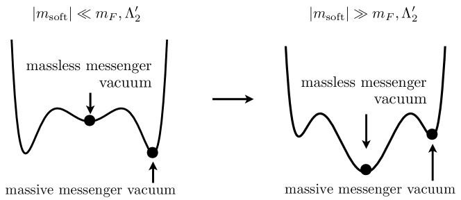
Figure 3: The possible phase transition into the massless messenger vacuum for $c_{SP}<0$. For too large $|m_{\rm soft}|$, the massive messenger vacuum becomes no more the global minimum of the potential.

5.1 Gravitino Mass

Let us now obtain a lower bound on the gravitino mass in this model. The fundamental scale of the SUSY breaking is bounded from below by the experimental limits on the sfermion masses, in particular the slepton masses [48],

$$m_{\tilde{\ell}}\gtrsim 94\,{\rm GeV}\ .$$ (56)

In our model we can convert this constraint into the lower bound on soft masses both in the primary and secondary SUSY sectors:

$$|m_{\rm soft}|\gtrsim 50\,{\rm TeV},~{}~{}~{}~{}|F_{S}|\gtrsim c_{SP}^{-1/2}\frac{m_{R}}{|m_{\rm soft}|}\times\left(50\,{\rm TeV}\right)^{2}\ ,$$ (57)

which in turn leads to a lower bound on the gravitino mass

$$m_{3/2}=\frac{F_{S}}{\sqrt{3}M_{\rm PL}}\gtrsim 0.6\,{\rm eV}\times c_{SP}^{-1/2}\frac{m_{R}}{|m_{\rm soft}|}\ .$$ (58)

We see that in the strong coupling limit (36) the gravitino can be as light as 1 eV.

Before closing this section, let us comment on the effective messenger number of this model. Messengers are composite fields transforming in the adjoint and fundamental representations of the Standard Model guage group. This could lead to the appearance of the Landau pole for the Standard Model gauge coupling below GUT scale [49]. In our model, however, composite messengers contribute to the renormalization group running of the gauge coupling constants in a interval between the scales $\mu_{R}\simeq m_{M,B}$ and $\mu_{R}\simeq\Lambda_{2}^{\prime}$. Thus, the effects from the composite messengers are very small for $m_{F}\sim\Lambda_{2}^{\prime}\sim|m_{\rm soft}|$. Above the the renormalization scale $\Lambda_{2}^{\prime}$, on the other hand, the model has only four fundamental representations of the $SU(5)_{\rm SM}$ gauge groups, and hence, the model allows perturbative coupling unification even for low SUSY breaking scale.

6 Conformal Gauge Mediation

The light gravitino mass can be achieved in the model of section 4 only if several a priori unrelated mass parameters are comparable. Here, we show that this apparent coincidence of scales may be a consequence of conformal symmetry of the underlying model (see Ref.[21] for the detailed discussion of conformal gauge mediation). Note that in the case where both gauge groups are asymptotically free, $N_{c}=2,3$, both $SP(N_{c})$ and $SU(4)$ are in conformal window. Thus, the existence of the IR conformal fixed point is plausible. At the fixed point, beta functions for gauge and Yukawa couplings must vanish leading to the following conditions

$$3(N_{c}+1)-(N_{c}+1)(1-\gamma_{Q})-4(1-\gamma_{R}) = 0\ ,$$ (59)

$$3\times 4-5(1-\gamma_{F})-2N_{c}(1-\gamma_{R}) = 0\ ,$$ (60)

$$\gamma_{S}+2\gamma_{Q} = 0\ .$$ (61)

These equations do not uniquely determine anomalous dimensions of the matter fields. To do so we use an $a$-maximization method [50]. The $a$-function of the model is given by,

$$a = 2N_{c}\cdot 2(N_{c}+1)\times(3(R_{Q}-1)^{3}-(R_{Q}-1))$$ (65)

$$+2N_{c}\cdot 2\cdot 4\times(3(R_{R}-1)^{3}-(R_{R}-1))$$

$$+10\cdot 4(3(R_{F}-1)^{3}-(R_{F}-1))$$

$$+(N_{c}+1)(2N_{c}+1)(3(R_{S}-1)^{3}-(R_{S}-1))\ ,$$

where $R_{i}$’s are related to the anomalous dimensions by $R_{i}=2(1+\gamma_{i}/2)/3$. The values of anomalous dimensions obtained both by using $a$-maximization method and perturbative one-loop calculation are presented in the table 3. We see a good agreement between the two calculations in the case $N_{c}=2$, strongly suggesting that a (relatively weakly coupled) fixed point exists. In the case $N_{c}=3$, the perturbative calculation breaks down but the existence of the IR fixed point is still plausible.

Table 3: Anomalous dimensions at the IR fixed point for $N_{c}=2,3$. Superscript $p$ denotes results of the perturbative calculation ($N_{c}=2$) while the superscript $a$ denotes results obtained by the $a$-maximization method. For $N_{c}=3$, the one-loop analysis does not give us meaningful comparison with the a-maximization method.

$N_{c}$	$\gamma_{Q}^{a}$	$\gamma_{Q}^{p}$	$\gamma_{R}^{a}$	$\gamma_{R}^{p}$	$\gamma_{F}^{a}$	$\gamma_{F}^{p}$	$\gamma_{S}^{a}$	$\gamma_{S}^{p}$
$2$	$-0.078$	$-0.062$	$-0.44$	$-0.45$	$-0.25$	$-0.24$	$0.16$	$0.12$
$3$	$-0.43$	$-$	$-0.57$	$-$	$0.48$	$-$	$0.86$	$-$

Let us now assume that, in the UV, the coupling constants are chosen close to the fixed point values while mass parameters $m_{R}$ and $m_{F}$ are small but non-vanishing. The model then quickly flows to the fixed point. and remains conformal down to scales of order $m_{R}$ (for $m_{R}>m_{F}$). Below $m_{R}$ conformal symmetry is broken and the low energy physics is that of cascade SUSY breaking. If the model is strongly coupled at the fixed point (as is suggested by the values of anomalous dimensions presented in the table 3), the scales of low energy $SP(N_{c})$ and $SU(4)$ dynamics are expected to be just below $m_{R}$,

$$m_{R}\sim\Lambda_{1}^{\prime}\sim\Lambda_{2}^{\prime}.$$ (66)

Notice that there is no arbitrariness in the relations between the mass scale $m_{R}$ and the dynamical scales since the values of the gauge coupling constants at around the energy scale $m_{R}$ are fixed by the conformal symmetry.

We still need one coincidence, namely IR values of $m_{R}$ and $m_{F}$ must be of the same order. It is reasonable to assume that these explicit mass scales are comparable in the UV, $m_{R}\sim m_{F}\sim m_{0}$. However, the effects of RG evolution are significant

$$m_{R} = m_{0}\times\left(\frac{m_{R}}{M_{\rm CFT}}\right)^{\gamma_{R}}\ ,$$ (67)

$$m_{F} = m_{0}\times\left(\frac{m_{R}}{M_{\rm CFT}}\right)^{\gamma_{F}}\ .$$ (68)

where $M_{\rm CFT}$ denotes the scale at which the model approaches the fixed point. Since $\gamma_{R}<\gamma_{F}$ we find that $m_{F}$ is naturally much smaller than $m_{R}$. As discussed in the appendix, the light gravitino scenario is still viable for small $m_{F}$ if $c_{SP}>0$.

Finally, we note that analysis of the gauge coupling unification becomes more involved in the case of conformal DSB sector. If the $SU(4)$ gauge coupling is closed to its fixed point value in a large interval of energy scales large anomalous dimensions of the messengers may have a significant effect on the running of MSSM gauge couplings (since the contribution of a single messenger to the beta function is changed by a factor of $(1-\gamma_{F})$). For $N_{c}=3$, the effective number of the messengers is smaller than four due to the large positive anomalous dimension of $F$, $\gamma_{F}=0.48$. For $N_{c}=2$, on the other hand, the number of messengers is enhanced and is just below five. Thus, careful studies are required to see whether the large anomalous dimensions cause the Landau pole problems below the GUT scale, when the scale $M_{\rm CFT}$ is close to the GUT scale. This problem can be avoided when the scale $M_{\rm CFT}$ is much lower than the GUT scale and the supersymmetry breaking sector is weakly coupled above $M_{\rm CFT}$.

Interestingly, when $M_{\rm CFT}$ is small compared to the GUT scale, it is also possible to relate the MSSM $\mu$-term with the mass parameter $m_{0}$ required in our model. If the CFT scale $M_{\rm CFT}=O(10^{10-13})$ GeV and we choose $\mu\sim m_{F}\sim m_{R}\sim m_{0}\sim(100)\,\mathrm{GeV}-O(1)\,\mathrm{TeV}$, then for $N_{c}=2$, the renormalization group evolution drives $m_{R}$ (and SUSY breaking scale) to the desired value of $m_{R}=O(10-100)$ TeV while $\mu$ remains at the electroweak scale (see also [21]).

7 Conclusions and discussion

In this paper, we proposed a new class of models with gauge mediated supersymmetry breaking, the cascade supersymmetry breaking, which admits a low scale gauge mediation and very light gravitino. This class of models is reminiscent of early GMSB models with several scales in that there is a primary and a secondary SUSY breaking sectors. However, in our model supersymmetry breaking in the secondary sector is itself achieved through gauge interactions. As we have demonstrated, it is possible to implement low scale gauge mediation in this class of models while avoiding light gaugino, Landau pole, and vacuum stability problems generic in direct GMSB models. Furthermore, a specific model presented in this paper may allow gravitino mass as low as to be as low as $O(1)$ eV, in the range that will be probed by the future cosmic microwave background observations [10].

Several comments are in order. As discussed in Refs.[51, 52, 53, 54], the models where messengers are charged under the strong gauge dynamics of the DSB sector generically suffer from the existence of the unwanted stable composite fields with MSSM quantum numbers. The model of section 4 possesses two global $U(1)$ symmetries (under which $F$ and $R$ fields are charged). Unless these symmetries are explicitly broken by higher dimensional terms in the Lagrangian, this implies existence of stable composite particles with masses in the range of tens to hundreds TeV. The annihilation cross-section for these particles may be close to the unitarity bound due to the strong interactions in the DSB sector. Nevertheless, stable composites charged under the Standard Model gauge group are severely constrained both by direct detection experiments and by the Bing Bang nucleosynthesis. For example, even the relic density of the neutral component $B$ and $\bar{B}$ with a mass in the hundreds TeV range is restricted to be lower than the observed dark matter density by a factor of $O(10^{-4})$  [55, 56]. Such a low relic density, however, cannot be achieved even when the annihilation cross section saturates the unitarity limit [57].

To avoid these constains, at least one global $U(1)$ must be broken explicitly. For example, if $B$ is the lightest composite with the Standard Model quantum numbers, the simplest operator that allows one to avoid direct detection constraints is  [54],

$$W=\frac{1}{M_{*}^{2}}\bar{F}\bar{F}\bar{F}\bar{F}\bar{5}_{\rm MSSM}\ ,$$ (69)

where $\bar{5}_{\rm MSSM}$ is the MSSM quarks and leptons in the $\bar{5}$ representation of $SU(5)_{\rm SM}$, and $M_{*}$ denotes the ultraviolet cutoff scale. Here, we have suppressed $SU(4)$ and $SU(5)_{\rm SM}$ indices. However, if the UV cutoff scale is as high as the GUT or the Planck scale, the lifetime of the composite messengers, is much longer than $1$ second and their decay may spoil the success of the Big Bang Nucleosynthesis (see Ref.[58] for recent constraints). If, on the other hand, $\bar{F}RQ$ is the lightest composite with the Standard Model quantum numbers, the $U(1)$ symmetry may be broken by a lower dimension operator

$$W=\frac{1}{M_{*}}F\bar{R}Q\bar{5}_{\rm MSSM}\ .$$ (70)

Since this operator is suppressed by only $M_{*}$, the resultant lifetime of the composite particle is much shorter than $1$ second.

A second global $U(1)$ symmetry allows the possibility that a neutral composite, $R^{4}$ or $\bar{R}^{4}$, is also stable. Such a composite provides a plausible dark matter candidate. Despite their large mass the the relic density of these particles can be consistent with observations since their annihilation cross section is expected to be close to the unitarity limit [57].

We would also like to note tha in the model of section 4 the continuous R-symmetry is broken down to the discrete $Z_{8}$ R-symmetry by the explicit mass terms in the secondary sector. Thus, the model does not have an R-axion even after the $X$ obtains non-vanishing vev. One exception is the choice of $c_{SP}>0$ which, as discussed in the appendix allows $m_{F}$ to be small compared to other mass scales in the theory (see table 2). In this case, the spontaneous breaking of an approximate continuous R-symmetry leads to a very light R-axion with mass

$$m_{a}^{2}\simeq\max\left[4m_{F}(\Lambda_{2}^{\prime}m_{\rm soft}^{2})^{1/3},\quad\sqrt{\frac{3}{5}}\frac{m_{3/2}^{2}M_{\rm PL}}{(\Lambda_{2}^{\prime}m_{\rm soft}^{2})^{1/3}}\right]\ .$$ (71)

Here, the second contribution comes from the explicit R-symmetry breaking by the constant term in the superpotential through the supergravity effects [59]. Therefore, it is possible that there is a very light R-axion with mass in the hundreds MeV range for $m_{F}=O(100)$ keV. Decay of such an axion inside the detector could lead to displaced vertex with a low-mass muon pair and be detactable at the LHC [60].

Finally, we would like to point out the primary SUSY breaking sector in the model of section 4 may give rise to pseudo Nambu-Goldstone bosons with mass in a TeV range. As disscussed in Refs. [61, 62] these particles may provide another plausible dark matter candidate. In this case, one can explain the observed excesses of cosmic ray electron/positron fluxes at PAMELA [63], ATIC [64], PPB-BETS [65], and Fermi [66] experiments, while evading the limit on anti-proton flux from PAMELA experiment [67].

Appendix A Cascade Supersymmetry breaking with $c_{SP}>0$

Analysis presented in the main text is valid independently of the sign of $c_{SP}$. However, in some perturbative models [5, 6, 7, 35], $c_{SP}$ is calculable and positive. If this is also the case in a strongly coupled regime of our model, a large region of the parameter space leads to viable superpartner spectrum.

This is a consequence of the fact that for positive $c_{SP}$ the phase transition to the vacuum at $X=0$ does not happen (see Fig.2) even for $(m_{F}^{3}\Lambda_{2}^{\prime})^{1/2}<m_{\rm soft}^{2}$. The vevs in the ground state are then largely shifted from the supersymmetric vevs in Eq.(31) to

$$\left\langle{X}\right\rangle \simeq \sqrt{10}(\Lambda_{2}^{\prime 2}m_{\rm soft})^{1/3}\left(1+\frac{{1}}{6}\left(\frac{m_{F}^{3}\Lambda_{2}^{\prime}}{m_{\rm soft}^{4}}\right)^{1/3}+\cdots\right)\ ,$$ (72)

$$F_{X} \simeq \frac{\sqrt{10}}{2}(\Lambda_{2}^{\prime 2}m_{\rm soft}^{4})^{1/3}\left(1-\frac{{1}}{3}\left(\frac{m_{F}^{3}\Lambda_{2}^{\prime}}{m_{\rm soft}^{4}}\right)^{1/3}+\cdots\right)\ ,$$ (73)

$$\frac{F_{X}}{\left\langle{X}\right\rangle} \simeq \frac{1}{2}m_{\rm soft}\left(1+\frac{{1}}{2}\left(\frac{m_{F}^{3}\Lambda_{2}^{\prime}}{m_{\rm soft}^{4}}\right)^{1/3}+\cdots\right)\ ,$$ (74)

and to leading order are independent of $m_{F}$ which is now a free parameter and, in particular, can be taken small. One must also verify that the messengers are non-tachyonic for positive $c_{SP}$. A detailed analysis of the messenger mass matrix shows that this is the case when

$$\Lambda_{2}^{\prime}\gtrsim m_{\rm soft}\ .$$ (75)

One advantage of the vacuum Eq.(72) is that the range of allowed values of $m_{F}$ is much larger while the gaugino and sfermion masses can be comparable without additional requirement $m_{F}\sim\Lambda_{2}\sim m_{\mathrm{soft}}$. In particular, if $c_{SP}$ is positive both low scale GMSB (if $\Lambda_{2}\sim m_{\mathrm{soft}}$) and high scale GMSB (if $\Lambda_{2}\gg m_{\mathrm{soft}})$ can be achieved where the gaugino and the sfermions masses are comparable (see table 2).

References

- [1] M. Dine, W. Fischler and M. Srednicki, Nucl. Phys. B 189, 575 (1981); S. Dimopoulos and S. Raby, Nucl. Phys. B 192, 353 (1981);
- [2] M. Dine and W. Fischler, Phys. Lett. B 110, 227 (1982); Nucl. Phys. B 204, 346 (1982); C. R. Nappi and B. A. Ovrut, Phys. Lett. B 113, 175 (1982); L. Alvarez-Gaume, M. Claudson and M. B. Wise, Nucl. Phys. B 207, 96 (1982);
- [3] S. Dimopoulos and S. Raby, Nucl. Phys. B 219, 479 (1983).
- [4] I. Affleck, M. Dine and N. Seiberg, Nucl. Phys. B 256, 557 (1985).
- [5] M. Dine and A. E. Nelson, Phys. Rev. D 48, 1277 (1993) [arXiv:hep-ph/9303230].
- [6] M. Dine, A. E. Nelson and Y. Shirman, Phys. Rev. D 51, 1362 (1995) [arXiv:hep-ph/9408384].
- [7] M. Dine, A. E. Nelson, Y. Nir and Y. Shirman, Phys. Rev. D 53, 2658 (1996) [arXiv:hep-ph/9507378].
- [8] See, for example, J. L. Feng, M. Kamionkowski, S. K. Lee, [arXiv:1004.4213 [hep-ph]].
- [9] M. Viel, J. Lesgourgues, M. G. Haehnelt et al., Phys. Rev. D71, 063534 (2005). [astro-ph/0501562].
- [10] K. Ichikawa, M. Kawasaki, K. Nakayama et al., JCAP 0908, 013 (2009). [arXiv:0905.2237 [astro-ph.CO]].
- [11] K. I. Izawa, Y. Nomura, K. Tobe and T. Yanagida, Phys. Rev. D 56, 2886 (1997) [arXiv:hep-ph/9705228].
- [12] C. Csaki, Y. Shirman and J. Terning, JHEP 0705, 099 (2007) [arXiv:hep-ph/0612241].
- [13] M. Dine and J. Mason, Phys. Rev. D 77, 016005 (2008) [arXiv:hep-ph/0611312].
- [14] S. Shirai, M. Yamazaki, K. Yonekura, JHEP 1006, 056 (2010). [arXiv:1003.3155 [hep-ph]].
- [15] See also a recent review, R. Kitano, H. Ooguri, Y. Ookouchi, [arXiv:1001.4535 [hep-th]], and references therein.
- [16] M. Ibe, K. Tobe, T. Yanagida, Phys. Lett. B615, 120-126 (2005). [hep-ph/0503098].
- [17] R. Sato and K. Yonekura, JHEP 1003, 017 (2010) [arXiv:0912.2802 [hep-ph]].
- [18] R. Sato, S. Shirai, [arXiv:1005.1255 [hep-ph]].
- [19] T. Aaltonen et al. [CDF Collaboration], Phys. Rev. Lett. 104, 011801 (2010) [arXiv:0910.3606 [hep-ex]].
- [20] J. Hisano, M. Nagai, S. Sugiyama et al., Phys. Lett. B665, 237-241 (2008). [arXiv:0804.2957 [hep-ph]].
- [21] M. Ibe, Y. Nakayama, T. T. Yanagida, Phys. Lett. B649, 292-298 (2007). [hep-ph/0703110 [HEP-PH]]; M. Ibe, Y. Nakayama, T. T. Yanagida, Phys. Lett. B668, 28-31 (2008). [arXiv:0802.2753 [hep-th]]; M. Ibe, Y. Nakayama, T. T. Yanagida, Phys. Lett. B671, 378-382 (2009). [arXiv:0804.0636 [hep-ph]].
- [22] D. Shih, JHEP 0802, 091 (2008). [hep-th/0703196 [HEP-TH]].
- [23] Z. Komargodski and D. Shih, JHEP 0904, 093 (2009) [arXiv:0902.0030 [hep-th]].
- [24] R. Sato and K. Yonekura, JHEP 1003, 017 (2010) [arXiv:0912.2802 [hep-ph]].
- [25] M. Ibe and R. Kitano, Phys. Rev. D 77, 075003 (2008) [arXiv:0711.0416 [hep-ph]].
- [26] A. Giveon, A. Katz and Z. Komargodski, JHEP 0907, 099 (2009) [arXiv:0905.3387 [hep-th]].
- [27] G. F. Giudice and R. Rattazzi, Nucl. Phys. B 511, 25 (1998) [arXiv:hep-ph/9706540].
- [28] M. Dine and J. D. Mason, Phys. Rev. D 78, 055013 (2008) [arXiv:0712.1355 [hep-ph]].
- [29] L. M. Carpenter, M. Dine, G. Festuccia et al., Phys. Rev. D79, 035002 (2009). [arXiv:0805.2944 [hep-ph]].
- [30] R. Sato, T. T. Yanagida, K. Yonekura, Phys. Rev. D81, 045003 (2010). [arXiv:0910.3790 [hep-ph]].
- [31] N. Seiberg, T. Volansky, B. Wecht, JHEP 0811, 004 (2008). [arXiv:0809.4437 [hep-ph]].
- [32] L. Randall, Nucl. Phys. B495, 37-56 (1997). [hep-ph/9612426].
- [33] K. -I. Izawa, T. Yanagida, Prog. Theor. Phys. 114, 433-437 (2005). [hep-ph/0501254].
- [34] M. Ibe, K. I. Izawa and Y. Nakai, Phys. Rev. D 80, 035002 (2009) [arXiv:0812.4089 [hep-ph]]; M. Ibe, K. I. Izawa and Y. Nakai, arXiv:0907.2970 [hep-ph].
- [35] Y. Nomura, K. Tobe and T. Yanagida, Phys. Lett. B 425, 107 (1998) [arXiv:hep-ph/9711220].
- [36] M. Fujii, M. Ibe and T. Yanagida, Phys. Rev. D 69, 015006 (2004) [arXiv:hep-ph/0309064].
- [37] T. Hotta, K. -I. Izawa, T. Yanagida, Phys. Rev. D55, 415-418 (1997). [hep-ph/9606203]
- [38] K. I. Izawa and T. Yanagida, Prog. Theor. Phys. 95, 829 (1996) [arXiv:hep-th/9602180]; K. A. Intriligator and S. D. Thomas, Nucl. Phys. B 473, 121 (1996) [arXiv:hep-th/9603158].
- [39] K. A. Intriligator and N. Seiberg, Nucl. Phys. B 431 (1994) 551 [arXiv:hep-th/9408155].
- [40] E. Witten, Nucl. Phys. B 202, 253 (1982).
- [41] Z. Chacko, M. A. Luty and E. Ponton, JHEP 9812, 016 (1998) [arXiv:hep-th/9810253].
- [42] N. Seiberg, Phys. Rev. D49, 6857-6863 (1994). [hep-th/9402044].
- [43] K. A. Intriligator, N. Seiberg and D. Shih, JHEP 0604, 021 (2006) [arXiv:hep-th/0602239].
- [44] M. Dine, F. Takahashi, T. T. Yanagida, [arXiv:1005.3613 [hep-th]].
- [45] E. Poppitz and S. P. Trivedi, Phys. Lett. B 401, 38 (1997) [arXiv:hep-ph/9703246].
- [46] N. Arkani-Hamed, G. F. Giudice, M. A. Luty et al., Phys. Rev. D58, 115005 (1998). [hep-ph/9803290].
- [47] P. Meade, N. Seiberg, D. Shih, Prog. Theor. Phys. Suppl. 177, 143-158 (2009). [arXiv:0801.3278 [hep-ph]].
- [48] C. Amsler et al. [Particle Data Group], Phys. Lett. B 667, 1 (2008).
- [49] J. L. Jones, Phys. Rev. D 79, 075009 (2009) [arXiv:0812.2106 [hep-ph]].
- [50] K. A. Intriligator and B. Wecht, Nucl. Phys. B 667, 183 (2003) [arXiv:hep-th/0304128].
- [51] K. Hamaguchi, S. Shirai and T. T. Yanagida, Phys. Lett. B 654, 110 (2007) [arXiv:0707.2463 [hep-ph]].
- [52] K. Hamaguchi, E. Nakamura, S. Shirai and T. T. Yanagida, Phys. Lett. B 674, 299 (2009) [arXiv:0811.0737 [hep-ph]].
- [53] K. Hamaguchi, E. Nakamura, S. Shirai and T. T. Yanagida, JHEP 1004, 119 (2010) [arXiv:0912.1683 [hep-ph]].
- [54] T. T. Yanagida, K. Yonekura, [arXiv:1006.2271 [hep-ph]].
- [55] Z. Ahmed et al. [The CDMS-II Collaboration], arXiv:0912.3592 [astro-ph.CO].
- [56] T. X. Collaboration, arXiv:1005.2615 [astro-ph.CO].
- [57] K. Griest, M. Kamionkowski, Phys. Rev. Lett. 64, 615 (1990).
- [58] M. Kawasaki, K. Kohri, T. Moroi, Phys. Rev. D71, 083502 (2005). [astro-ph/0408426].
- [59] J. Bagger, E. Poppitz, L. Randall, Nucl. Phys. B426, 3-18 (1994). [hep-ph/9405345].
- [60] H. -S. Goh, M. Ibe, JHEP 0903, 049 (2009). [arXiv:0810.5773 [hep-ph]].
- [61] M. Ibe, Y. Nakayama, H. Murayama et al., JHEP 0904, 087 (2009). [arXiv:0902.2914 [hep-ph]].
- [62] M. Ibe, H. Murayama, S. Shirai et al., JHEP 0911, 120 (2009). [arXiv:0908.3530 [hep-ph]].
- [63] O. Adriani et al. [PAMELA Collaboration], Nature 458, 607 (2009) [arXiv:0810.4995 [astro-ph]].
- [64] J. Chang et al., Nature 456, 362 (2008).
- [65] S. Torii et al., arXiv:0809.0760 [astro-ph].
- [66] A. A. Abdo et al. [The Fermi LAT Collaboration], arXiv:0905.0025 [astro-ph.HE].
- [67] O. Adriani et al., Phys. Rev. Lett. 102, 051101 (2009) [arXiv:0810.4994 [astro-ph]].
- [68] Y. Nomura, J. Thaler, Phys. Rev. D79, 075008 (2009). [arXiv:0810.5397 [hep-ph]].
- [69] J. Mardon, Y. Nomura, D. Stolarski et al., JCAP 0905, 016 (2009). [arXiv:0901.2926 [hep-ph]].
- [70] J. Mardon, Y. Nomura, J. Thaler, Phys. Rev. D80, 035013 (2009). [arXiv:0905.3749 [hep-ph]].