Optimistic limits of the colored Jones polynomials
Abstract
We show that the optimistic limits of the colored Jones polynomials of the hyperbolic knots coincide with the optimistic limits of the Kashaev invariants modulo .
1 Introduction
1.1 Preliminaries
Kashaev conjectured the following relation in [5] :
where is a hyperbolic link, vol() is the hyperbolic volume of , and is the -th Kashaev invariant. After, a generalized conjecture was proposed in [12] that
where cs() is the Chern-Simons invariant of defined in [7].
The calculation of the actual limit of the Kashaev invariant is very hard, and only several cases are known. On the other hand, while proposing the conjecture, Kashaev used a formal approximation to predict the actual limit. His formal approximation was formulated as optimistic limit by H. Murakami in [9]. This method can be summarized in the following way. First, we fix an expression of , then apply the following formal substitution
| (1) | |||||
to the expression, where , for , is the residue of an integer modulo , and . Then by substituting each with a complex variable , we obtain a potential function . Finally, let
and evaluate for an appropriate solution of the equations . Then the resulting complex number is called the optimistic limit.
For example, the optimistic limit of the Kashaev invariant of the knot was calculated in [5] and [13] as follows. By the formal substitution,
By substituting and , we obtain
and
For the choice of a solution of the equations , the optimistic limit becomes
As seen above, the optimistic limit depends on the expression and the choice of the solution, so it is not well-defined. However, Yokota made a very useful way to determine the optimistic limit of a hyperbolic knot in [17] and [18] by defining a potential function of the knot diagram, which also comes from the formal substitution of certain expression of the Kashaev invariant (the definition of will be given in Section 3.1). As above, he also defined
and
After proving that is the hyperbolicity equation of Yokota triangulation, he chose the geometric solution of (Yokota triangulation will be discussed in Section 2.1. The hyperbolicity equation consists of edge relations and the cusp conditions of a triangulation, and the geometric solution is the one which gives the hyperbolic structure of the triangulation. Details are in Section 4). Then he proved
| (2) |
in [18]. Therefore, we denote
and call it the optimistic limit of the Kashaev invariant .
To obtain (2), Yokota assumed several assumptions on the knot diagram and the existence of an essential solution of . The assumptions on the diagram essentially mean to reduce redundant crossings of the diagram before finding the potential function . Exact statements are Assumption 1.1–1.4. and Assumption 2.2. in [18]. We remark that these assumptions are needed so that, after the collapsing process, Yokota triangulation becomes a topological triangulation of the knot complement (see Section 3.1 for details).
As mentioned before, the set of equations becomes the hyperbolicity equation of Yokota triangulation. Therefore, each solution of determines the shape parameters of the ideal tetrahedra of the triangulation and the parameters are expressed by the ratios of (details are in Section 4). We call a solution of essential if no shape parameters are in , which implies no edges of the triangulation are homotopically nontrivial. A well-known fact is that if the hyperbolicity equation has an essential solution, then there is a unique geometric solution of (for details, see Section 2.8 of [16]). Therefore, to guarantee the existence of the geometric solution, Yokota assumed the existence of an essential solution.
On the other hand, it is proved in [11] that
where is the -th colored Jones polynomial of the link with a complex variable . Therefore, it is natural to define the optimistic limit of the colored Jones polynomial so that it gives the volume and the Chern-Simons invariant. Although it looks trivial, due to the ambiguity of the optimistic limit, only few results are known. It was numerically confirmed for few examples in [12], actually proved only for the volume part of two bridge links in [13] and for the Chern-Simons part of twist knots in [2]. In a nutshell, the purpose of this paper is to propose a general method to define the optimistic limit of the colored Jones polynomial of a hyperbolic knot and to prove the following relation :
| (3) |
1.2 Main result
For a hyperbolic knot , we define a potential function of a knot diagram in Section 3.2, which also comes from the formal substitution of certain expression of the colored Jones polynomial . We define
and
Also, we discuss Thurston triangulation of the knot complement in Section 2.2, which was introduced in [14].
Proposition 1.1.
For a hyperbolic knot with a fixed diagram, we assume the diagram satisfies Assumption 1.1.–1.4. and Assumption 2.2. in [18]. For the potential function of the diagram, becomes the hyperbolicity equation of Thurston triangulation.
Each solution of determines the shape parameters of the ideal tetrahedra of Thurston triangulation and the parameters are expressed by the ratios of (details are in Section 4). We call a solution of essential if no shape parameters are in . Comparing Yokota triangulation and Thurston triangulation, we obtain the following Lemma.
Lemma 1.2.
For a hyperbolic knot with a fixed diagram and the assumptions of Proposition 1.1, an essential solution of determines the unique solution of , and vice versa. Furthermore, if the determined solution is essential, then also induces , and vice versa.
Proof of Lemma 1.2 will be given in Section 5. Although there is a possibility that an essential solution of determines a non-essential solution of , we expect this not to happen in almost all cases (this is discussed in Appendix A.2). In this paper, we only consider the case when the determined solution is essential.
Theorem 1.3.
For a hyperbolic knot with a fixed diagram, assume the assumptions of Proposition 1.1. Let and be the potential functions of the knot diagram. Also assume the hyperbolicity equation has an essential solution and let be the geometric solution of . From Lemma 1.2, let and be the corresponding solutions of determined by and by , respectively. We also assume and are essential. Then
-
1.
-
2.
is the geometric solution of and
The proof is in Section 5. We denote
and call it the optimistic limit of the colored Jones polynomial . With this definition, Theorem 1.3 implies (3). Also, we obtain the colored Jones polynomial version of Corollary 1.4 of [1] as follows.
Corollary 1.4.
For a hyperbolic knot with a fixed diagram, assume the assumptions of Proposition 1.1. Let be an essential solution of , be the geometric solution of , and be the parabolic representation induced by . Also, assume the corresponding solutions and of , determined by and by , respectively, from Lemma 1.2 are essential. Then
where is the complex volume of defined in [19]. Furthermore, the following inequality holds:
| (4) |
The equality in (4) holds if and only if .
Proof.
It is a well-known fact that the hyperbolic volume is the maximal volume of all possible representations and that the maximum happens if and only if the representation is discrete and faithful (for the proof and details, see [4]).
From the proof of Lemma 1.2, if and are essential, then the shapes of each (collapsed) octahedra in Figure 2 and Figure 10 of Yokota and Thurston triangulations coincide. Therefore, these triangulations form the same geometric shape, and the parabolic representation coincides with up to conjugate, where and are the parabolic representations induced by and by , respectively. This also implies that is the geometric solution of .
Yokota proved
in [18] using Zickert’s formula of [19], but the formula also holds for any parabolic representation induced by . Therefore, Yokota’s proof also implies
Among the essential solutions of , only the geometric solution induces the discrete faithful representation. Therefore, applying Theorem 1.3, we complete the proof.
∎
This paper consists of the following contents. In Section 2, we describe Yokota triangulation and Thurston triangulation, which correspond to the Kashaev invariant and the colored Jones polynomial, respectively. We show that these two triangulations are related by finite steps of 3-2 moves and 4-5 moves on some crossings. In Section 3, the potential functions and are defined. In Section 4, we explain the geometries of and , and prove Proposition 1.1. In Section 5, we introduce several dilogarithm identities and complete the proofs of Lemma 1.2 and Theorem 1.3 using these identities. In Appendix A.1, we show the potential function defined in Section 3 can be obtained by the formal substitution of the colored Jones polynomial. Finally, in Appendix A.2, we investigate the necessary and sufficient condition for an essential solution of (respectively, ) to induce the inessential solution of (respectively, ).
2 Two ideal triangulations of the knot complement
In this section, we explain two ideal triangulations of the knot complement. One is Yokota triangulation corresponding to the Kashaev invariant in [18] and the other is Thurston triangulation corresponding to the colored Jones polynomial in [14]. A good reference of this section is [10], which contains wonderful pictures.
2.1 Yokota triangulation

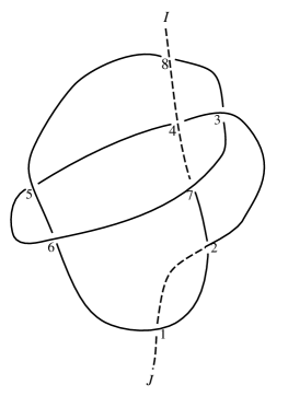
Consider a hyperbolic knot and its diagram (see Figure 1(a)). We define sides of as arcs connecting two adjacent crossing points. For example, Figure 1(a) has 16 sides.
Now split a side of open so as to make a (1,1)-tangle diagram and label crossings with integers (see Figure 1(b)). Yokota assumed several conditions on this (1,1)-tangle diagram (for the exact statement, see Assumption 1.1.–1.4. and Assumption 2.2. in [18]). The assumptions roughly mean that we remove all the crossing points that can be reduced trivially. Also, let the two open sides be and and consider the orientation from to . Assume and are in an over-bridge and in an under-bridge, respectively (Over-bridge is a union of sides, following the orientation of the knot diagram, from one over-crossing point to the next under-crossing point. Under-bridge is the one from one under-crossing point to the next over-crossing point. The boundary endpoints of and are considered over-crossing point and under-crossing point, respectively. For example, in Figure 1(b), if we follow the diagram from the below to the top, the first under-bridge containing ends at the crossing 2, and the first over-bridge starts at the crossing 2 and ends at the crossing 4. In total, it has 5 over-bridges and 5 under-bridges. Note that if we change the orientation, the numbers of over-bridges and under-bridges change).
Now extend and so that, when following the orientation of the knot diagram, non-boundary endpoints of and become the last under-crossing point and the first over-crossing point, respectively, as in Figure 1(b). Then we assume the two non-boundary endpoints of and do not coincide, because, if they coincide, then we cut other side open and make a different tangle diagram. Yokota proved in [18] that we can always make two non-boundary endpoints different by cutting certain side open because, if not, then the diagram should be that of a link or the trefoil knot (for details, see Assumption 1.3. and the discussion that follows in [18]).
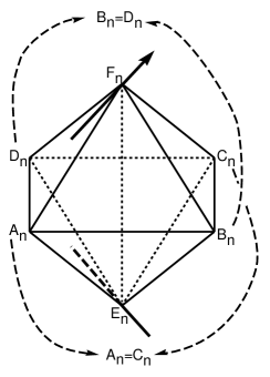
To obtain an ideal triangulation of the knot complement, we place an ideal octahedron on each crossing as in Figure 2(a). We call the edges , , and of the octahedron horizontal edges. Figure 2(b) shows the positions of , , , and the horizontal edges. We twist the octahedron by identifying the edges to and to as in Figure 2(a) (the actual shape of the resulting diagram appears in [10]). Then we glue the faces of the twisted octahedron following the knot diagram. For example, in Figure 2(b), we glue to , to , to , to , and so on. Finally, we glue to . Note that, by gluing likewise, all and are identified to one point, all and are identified to another point, and all and are identified to yet another point. Let these points be , and , respectively. Then the regular neighborhoods of and become 3-balls, whereas that of becomes the tubular neighborhood of the knot .
We split each octahedron into four tetrahedra, , , and . Then we collapse faces that lie on the split sides. For example, in Figure 2(b), we collapse the faces and to different points. Note that this face collapsing makes some edges on these faces into points. Actually, the non-horizontal edges , , , , and the horizontal edges , , , in Figure 2(b) are collapsed to points because of the face collapsing. This makes the tetrahedra , , , , , , , , , , , , , , , , , , and be collapsed to points or edges.

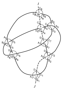
The surviving tetrahedra after the collapsing can be depicted as follows. First, remove and on the tangle diagram and denote the result as (see Figure 3). Note that, by removing , some vertices are removed, two vertices become trivalent and some sides are glued together. In Figure 3, vertices 1, 4, 8 are removed, 2, 7 become trivalent and has 9 sides (we consider the sides at the trivalent vertices are not glued together). Now we remove the horizontal edges on the removed vertices, the horizontal edges that are adjacent to and the horizontal edges in the unbounded region (see Figure 3 for the result). The surviving horizontal edges mean the surviving ideal tetrahedra after the collapsing. In the example, 12 tetrahedra survive.
The collapsing identifies the points , , and to each other and connects the regular neighborhoods of them. Collapsing certain edges of a tetrahedron may change the topological type of , but Yokota excluded such cases by Assumption 1.1.–1.3. on the shape of the knot diagram. (Assumption 1.1.–1.2. roughly means the diagram has no redundant crossings and Assumption 1.3. means the two non-boundary endpoints of and do not coincide.) Therefore, the result of the collapsing makes the neighborhood of to be the tubular neighborhood of the knot, and we obtain the ideal triangulation of the knot complement (see [18] for a complete discussion).
2.2 Thurston triangulation
Thurston triangulation, introduced in [14], uses the same octahedra and the same collapsing process, so it also induces an ideal triangulation of the knot complement. However, it uses a different subdivision of each octahedra. In Figure 2(a), Yokota triangulation subdivides each octahedron into four tetrahedra. However, Thurston triangulation subdivides it into five tetrahedra, , , , and (see the right-hand side of Figure 4(a) for the shape of the subdivision). In this subdivision, if we apply the collapsing process, then some pair of tetrahedra shares the same four vertices (see the first case of (Case 2) in the proof of Observation 2.1 for an example). For the convenience of discussion, when this happens, we remove these two tetrahedra and call the result Thurston triangulation.
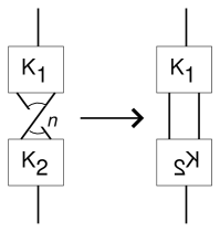
To see the relation between these two triangulations, we define 4-5 move of an octahedron and 3-2 move of a hexahedron as in Figure 4.
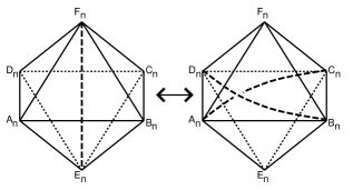

Before the collapsing process, two triangulations are related by only 4-5 moves on each crossings. However, the following observation shows they are actually related by 4-5 moves and also by 3-2 moves on some crossings after the collapsing.
Observation 2.1.
For a hyperbolic knot with a fixed diagram, if the diagram satisfies Assumption 1.1.–1.4. and Assumption 2.2. in [18], then Yokota triangulation and Thurston triangulation are related by 3-2 moves and 4-5 moves on some crossings.
Proof.
First, for a non-trivalent vertex of , we show only one horizontal edge in Figure 2(a) can be collapsed. If any of two horizontal edges are collapsed, then the (1,1)-tangle diagram should be Figure 5(a) or Figure 5(b) for some tangle diagrams or because the collapsed edges should lie in the unbounded regions. However, Figure 5(a) is excluded because, if we close up the open side, then and cannot be prime. We can also exclude Figure 5(b) because it violates Assumption 1.1. in [18]. Actually, in the later case, we can reduce the number of crossings as in Figure 5(b).
Because of this and Yokota’s Assumptions, all possible cases of collapsing edges in Figure 2(a) are as follows :
(Case 1) if is a non-trivalent vertex of , then none or one of the horizontal edges is collapsed.
(Case 2) if is a trivalent vertex of , then
-
1.
is collapsed and none or one of , is collapsed,
-
2.
is collapsed and none or one of , is collapsed,
-
3.
is collapsed and none or one of , is collapsed.
(Case 1) is trivial, so we consider the first case of (Case 2).
If and are collapsed, then the survived tetrahedron is in Yokota triangulation, and in Thurston triangulation. They coincide because by the collapsing of .
If is collpased and no others are, then the survived tetrahedra are and in Yokota triangulation, and , , and in Thurston triangulation. However, in Thurston triangulation, two tetrahedra and cancel each other because they share the same vertices , , and . The others coincide with the tetrahedra in Yokota triangulation because .
Other cases of (Case 2) are the same as the first case, so the proof is completed.
∎
3 Potential functions
3.1 The case of Kashaev invariant
In the case of Kashaev invariant, Yokota’s potential function is defined by the following way.
For the graph , we define contributing sides as sides of which are not on the unbounded regions. For example, there are 5 contributing sides and 4 non-contributing sides in Figure 6. We assign complex variables to contributing sides and real number 1 to non-contributing sides. Then we label each ideal tetrahedra with and assign () to the horizontal edge of as the shape parameter. We define as the counterclockwise ratio of the complex variables .
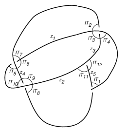
For example, in Figure 6,
For each tetrahedron , we assign dilogarithm function as in Figure 7. Then we define by the summation of all these dilogarithm functions. We also define the sign of by
Then is expressed by
For example, in Figure 6,
and
3.2 The case of colored Jones polynomial
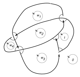
For each region of , we choose one bounded region and assign 1 to it. Then we assign variables to the remaining bounded regions, and 0 to the unbounded region (see Figure 8).
For each vertex of , we assign the following functions according to the type of the vertex and the horizontal edges. For positive crossings :
For negative crossings :
If no horizontal edge is collapsed at the positive nor the negative crossing, we assign any of or to the crossing, respectively. In Lemma 3.1, we will show this choice does not have any effect on the optimistic limit of the colored Jones polynomial.
For the endpoints of and , we use the same formula disregarding whether certain horizontal edge is collapsed or not. For the endpoint of :
For the endpoint of :
In Appendix, we show that the assigned functions above are, in fact, obtained by the formal substitution of certain forms of the R-matrix of the colored Jones polynomial.
Now we define the potential function of the knot diagram by the summation of all functions assigned to the vertices of . For example, the potential function of Figure 8 is
| (5) | |||
We end this section with the invariance of the optimistic limit under the choice of the four different forms of the potential functions of a crossing.
Lemma 3.1.
For the functions defined above, let
Then
and for ,
Proof.
For a given complex-valued function , let
| (6) |
for some integer constants . Then by a direct calculation,
and
These show and define the same optimistic limit, so we define an equivalence relation by for and satisfying (6).
For
using the well-known identity for in [6], we obtain
For any integer , some integers and indices , we have
and
Therefore, we obtain
Other equalities and can be obtained by the same method or by the symmetry of the equations. ∎
4 Geometric structures of the triangulations
For Yokota triangulation and Thurston triangulation, we assign complex variables to each tetrahedra and solve certain equations. Then one of the solutions gives the complete hyperbolic structure of the knot complement. We describe these procedures in this section.
First, consider the positive and negative crossings in Figure 9, where are the variables assigned to the sides of and are the variables assigned to the regions of . Note that and are used for defining the potential functions and , respectively.
Then consider Figure 10. We assign , to the horizontal edges , , , , respectively. This assignment determines the shape parameters of the tetrahedra of Yokota triangulation. Also, for the positive crossing, we assign , , , to , , , , respectively, and assign to and for the parameter of the tetrahedron . For the negative crossing, we assign , , , to , , , , respectively, and assign to and for the parameter of the tetrahedron . These assignments determine the shape parameters of the tetrahedra of Thurston triangulation.
We do not assign any shape parameters to the collapsed edges. Also, in the case of Thurston triangulation, we do not assign any shape parameters to the edges that contain the endpoints of the collapsed edges. For example, if is collapsed, then we do not assign any shape parameters to , nor . Also, if is collapsed in Figure 10(a), then we do not assign any shape parameters to , , nor .222 The edges and are horizontal edges, but are identified to non-horizontal edges. When this happens, we do not assign shape parameters to these edges.
Yokota and Thurston triangulations are ideal triangulations, so by assigning shape parameters, we can determine all the shapes of the hyperbolic ideal tetrahedra of the triangulations. Note that if we assign a shape parameter to an edge of an ideal tetrahedron, then other edges are also parametrized by and as in Figure 11.
So as to get the hyperbolic structure, these shape parameters should satisfy the edge relations and the cusp conditions. The edge relations mean the product of all shape parameters assigned to each edge should be 1, and the cusp conditions mean the holonomies induced by the longitude and the meridian should be translations on the cusp. These two conditions can be expressed by a set of equations of the shape parameters, and we call this set of equations hyperbolicity equations (for details, see Chapter 4 of [15]). We call a solution of the hyperbolicity equations of Yokota triangulation essential if none of the shape parameters of the tetrahedra are one of . We also define an essential solution of Thurston triangulation in the same way. It is a well-known fact that if the hyperbolicity equations have an essential solution, then they have the unique solution which gives the hyperbolic structure to the triangulation333 Strictly speaking, we have unique values of shape parameters. However, these values uniquely determine the solutions and . This was explained in [18] for Yokota triangulation, which will be at the end of this section for Thurston triangulation. (for details, see Section 2.8 of [16]). We call this unique solution the geometric solution, and denote the geometric solution of Yokota triangulation by and that of Thurston triangulation by We remark that, in Theorem 1.3, we assumed the existence of the geometric solutions and .
Yokota proved in [18] that, for the potential function defined in Section 3.1,
becomes
the hyperbolicity equations of Yokota triangulation.
In other words, each element of
becomes an edge relation or a cusp condition
for all , and all other equations are trivially induced from the elements of .
Proposition 1.1 shows the same holds for the potential function defined in Section 3.2 and . We prove this in this section.
Let be the set of non-collapsed horizontal edges of Thurston triangulation of . Let be the set of non-collapsed non-horizontal edges , , , , , , , in Figure 10, which are not in .444 Collapsing may identify some horizontal edges to non-horizontal edges. In this case, we put these identified edges in . Finally, let be the set of edges , in Figure 10, which are not in .
For example, in Figure 3, , , , , , , , , and .
Lemma 4.1.
For a hyperbolic knot with a fixed diagram, we assume the assumptions of Proposition 1.1. Then the edges in satisfy the edge relations trivially by the assigning rule of the shape parameters.
Proof.
If an edge or of Figure 10 is in , then the octahedron does not have any collapsed edge. By the assigning rule of the shape parameters, all the edges in satisfy edge relations trivially.
Now we show the case of . Consider the following four cases of two points and in Figure 12 and the two regions between the crossings parametrized by the variables and (for the positions of the points , see Figure 2). First, we assume no edges are collapsed in the tetrahedra and . This means the two regions with and in Figure 12 are bounded.
In the case of Figure 12(a), we want to prove that the edge relation of the edge holds trivially. We draw a part of the cusp diagram in near as in Figure 13. Our tetrahedra are all ideal, so the triangles and are Euclidean. Note that are points in the edges , , , , , respectively. Furthermore, edges and are identified to and to , respectively.555 In fact, edges and are also identified, so the two triangles are cancelled by each other. This means the corresponding tetrahedra and are cancelled by each other. On the edge , two shape parameters and are assigned respectively by the assigning rule, so the edge relation of holds trivially.
In the case of Figure 12(c), we want to prove that the edge relation of holds trivially. If is a positive crossing, then we draw a part of the cusp diagram in near , and if is a negative crossing, then we draw a part of the cusp diagram in near as in Figure 14.
Note that if is a positive crossing, then are points in the edges , , , , respectively, and if is a negative crossing, then are points in the edges , , , , respectively. Furthermore, the edge is identified to , so the diagram in Figure 14 becomes an annulus. The product of shape parameters around in the annulus is , and the one around is also . Therefore, if we consider the previous annulus on the right of Figure 14, which shares the edge , then we obtain the edge relation of trivially.
We remark that the previous annulus always exists because, when we follow the horizontal line in Figure 12(c) backwards, after meeting the under-crossing point , we let the next over-crossing point (see Figure 15). (If does not exist, then but this violates our assumption.) Then a part of the cusp diagram between and also forms an annulus, and this is the previous annulus.666 As we have seen in the case of Figure 12(a), the crossing points between and do not have any effect on the part of the cusp diagram because the triangles in Figure 13 are cancelled by each other. Also, as explained below, the existence of the previous annulus still holds even if some regions between and are unbounded.
The cases of Figure 12(b) and Figure 12(d) are the same as the cases of Figure 12(a) and Figure 12(c), respectively. Therefore, we find all the edges in satisfy the edge relations trivially by the method of parametrizing edges.
Now we assume one of the regions parametrized by or in Figure 12 is an unbounded region. Then the cusp diagram in Figure 13 collapses to an edge and the one in Figure 14 collapses to an edge . Therefore, our arguments for still hold for the collapsed case.777 What we need is to consider the next annuli on the left and the right side, and do the same arguments.
∎
Proof of Proposition 1.1.
Consider the function , which previously appeared in Section 3.2. By direct calculation, we obtain
| (7) | |||||
| (8) | |||||
| (9) | |||||
| (10) |
Note that (7), (8), (9) and (10) are the products of shape parameters assigned to the edges , , and of Figure 10(a), respectively.888 For example, consider equation (7) and Figure 10(a). The shape parameters assigned to the edge are , and , which come from the tetrahedra , and , respectively. Also, after evaluating to , we obtain
| (11) | |||||
| (12) | |||||
| (13) |
Note that (11), (12) and (13) are the products of shape parameters assigned to the edges , and of Figure 10(a), respectively, after collapsing the edge . Direct calculation shows the same relations hold for , , , , , and .
Consider the first potential function for the end point of in Section 3.2. Direct calculation shows
| (14) | |||||
| (15) | |||||
| (16) | |||||
| (17) | |||||
| (18) |
where (14) and (15) are the products of shape parameters assigned to the edges and of Figure 10(a), respectively, after collapsing the edge without or with the collapsing of a horizontal edge.
To explain that (16), (17) and (18) are still parts of edge relations, we need different arguments. First, consider Figure 16.
In Figure 16(a), the product of all shape parameters assigned to the edge expressed by dots is
| (19) |
and in Figure 16(b), the product is
| (20) |
To see the meaning of (16), consider the following two cases in Figure 17, where is the end point of and is the previous over-crossing point. Figure 17(a) means the case when there is no crossing point between and , and Figure 17(b) means the other case.
Because is the endpoint of , the edge of the octahedron on in Figure 10(a) is collapsed to a point and becomes two tetrahedra as in Figure 18 (if one more horizontal edge is collapsed here, the result becomes one tetrahedron. This is the cases of equations (17) and (18)).
The part of the cusp diagrams for each case are in Figure 19 (see Figure 9 and Figure 10 for the assigning rule of the shape parameters).
In the case of Figure 17(a), the product of shape parameters assigned to the edges of Figure 18 is . These edges are identified to , and is assigned to this edge. This explains that (16) is the product of shape parameters assigned to the edges .
In the case of Figure 17(b), the product of shape parameters assigned to the edges of Figure 18 is . In Figure 19(b), these edges are identified to the edges drawn by the dots, and the product of shape parameters assigned to the edges is
by (19) and (20). This also explains (16) is the product of shape parameters assigned to and some other edges identified to this. This fact is still true999 Even if the endpoint of lies between the crossings and , this fact is still true because the collapsing of the non-horizontal edges does not change the part of the cusp diagram we are considering. even if some of the regions assigned by are unbounded regions because the collapsing of the horizontal edges makes the cusp diagrams of Figure 13 and Figure 14 into edges. If the cusp diagram of Figure 13 becomes an edge, then ignoring the diagram is enough for our consideration, and if that of Figure 14 becomes an edge, then considering the previous annulus is enough. The previous annulus always exists because, by the same argument as in the proof of Lemma 4.1, if we choose the next over-crossing point by following the horizontal lines backwards, the cusp diagram between and becomes the previous annulus.101010 There is a concern that the previous annulus is collapsed to an edge, and all the previous annuli, following the horizontal line, are collapsed to edges. However, this cannot happen because Thurston triangulation is a triangulation of the hyperbolic knot complement and we assumed the existence of the geometric solution.
Now we describe the meaning of (17). Let be the end point of , be the previous over-crossing point and be the previous under-crossing point. Also let be the previous point of . Assume the edges and of Figure 10(a) are collapsed. Then , and is assigned to this edge. If , then the edges identified to appear between the points and as the dots in Figure 16, and if , then the edges appear between and in the same way. Particularly, Figure 16(a) may appear many times, but Figure 16(b) appears only one time at the points or , respectively. By (19) and (20), the product of all shape parameters assigned to the dots is , so (17) is the product of shape parameters assigned to the edges and some others identified to these. This fact is still true when some of the horizontal edges or non-horizontal edges of the octahedra are collapsed because of the same reason explained above for the case of (16).
The same relations hold for (18) and the cases of other potential functions of the endpoints of and by the same arguments.
Therefore, we conclude that becomes all the edge relations of except the one horizontal edge whose region is assigned as 0 instead of the variables . For an ideal tetrahedron parametrized with as in Figure 11, the product of all shape parameters assigned to all edges in the tetrahedron is . This implies the product of all edge relations becomes 1. On the other hand, from Lemma 4.1 and the above arguments, we found all but one edge relation by . Therefore, the remaining edge relation holds automatically.
Finally, we prove contains the cusp condition. Note that edges and in Figure 14 are meridians of the cusp diagram. The same shape parameter is assigned to the corners and , so one of the cusp conditions is trivially satisfied by the method of assigning shape parameters to edges. If we have all the edge relations and one cusp condition of a meridian, then we can obtain all remaining cusp conditions using these relations. Therefore, we conclude are the hyperbolicity equations of Thurston triangulation of .
∎
We remark one technical fact. For Thurston triangulation, let the shape parameters of the ideal tetrahedra be . These parameters are defined by the ratios of a solution of , so if the values of are fixed, then the values of are uniquely determined and satisfy the hyperbolicity equation. Likewise, if the values of satisfying the hyperbolicity equations are fixed, then we can uniquely determine the solution of of as follows: First, we can determine some of the values of , which are assigned to the regions adjacent to the region assigned with the number 0. Once a value of a region is determined, then all the values of the adjacent regions can be determined. Therefore, all can be determined. Furthermore, those values are well-defined and become a solution of because of the hyperbolicity equations.
In the next section, we will show the shape parameters of Yokota triangulation determines that of Thurston triangulation, and with certain restriction, vice versa. By the above discussion, this correspondence means each essential solution of determines a unique solution of . Furthermore, if all the determined solutions of are essential, then each essential solution of determines a unique essential solution of .
5 Proof of Theorem 1.3
We start this section with the proof of Lemma 1.2.
Proof of Lemma 1.2.
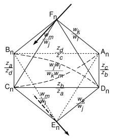
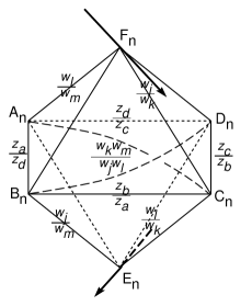
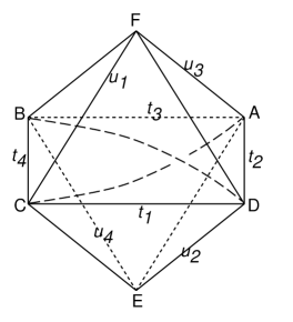
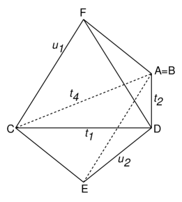
For a hyperbolic ideal octahedron in Figure 20, we assign shape parameters , , , , , , and to the edges CD, DA, AB, BC, CF, DE, AF and BE, respectively. Let , which is also a shape parameter assigned to the edges AC and BD of the tetrahedron ABCD.
Then we obtain the following relations.
| (31) |
Note that and are the shape parameters of the tetrahedra in Yokota triangulation and in Thurston triangulation, respectively. According to Observation 2.1, we know these two triangulations are related by 3-2 moves and 4-5 moves on collapsed octahedra and non-collapsed octahedra, respectively. Equation (31) shows the correspondence between the shape parameters under 4-5 moves, so if , then we can determine the values of from the left side of (31). Also the equation corresponding to 3-2 move can be obtained easily (see (56) for example). This implies that the shape parameters of Yokota triangulation determine that of Thurston triangulation. Furthermore, if all , then the shape parameters of Thurston triangulation recover that of Yokota triangulation by the right side of (31). This completes the proof.
∎
Our goal of this section is to prove
for any essential solution of and the corresponding essential solution of . To prove this, we introduce the dilogarithm identities of an ideal octahedron in Lemma 5.1. Note that the functions and are multi-valued functions. Therefore, to obtain well-defined values, we have to select a proper branch of the logarithm by choosing and .
Let be the Bloch-Wigner function for . It is a well-known fact is invariant under any choice of log-branch and that , where is the hyperbolic ideal tetrahedron with the shape parameter . Therefore, from Figure 20, we obtain
| (32) |
Lemma 5.1.
Let be the shape parameters defined in the hyperbolic octahedron in Figure 20 satisfying (31) and (32). Then the following identities hold for any choice of log-branch.
Furthermore,
when AB is collapsed to a point,
when BC is collapsed to a point,
when CD is collapsed to a point, and
when DA is collapsed to a point.
Proof.
For a function consisting of dilogarithms and logarithms with certain fixed log-branch, we denote by the same function with different log-branch corresponding to an analytic continuation of . It is a well-known fact that
| (41) |
for certain integer . Let . Then using (41), we have
and
| (42) |
Similarly, for , we have
| (43) |
First, we will prove is invariant modulo for any choice of log-branch by showing
| (46) |
Note that
From (31), we know
Therefore, from (5) and the above, we have
Combining (5) and (5), we obtain
From (31), we know
and
Applying (44) and (45) to (5), we obtain
which shows (46).
Now we will prove for certain log-branch. Direct calculation shows the imaginary part of (5.1) becomes
Using , we obtain
By applying these, we can verify the imaginary part of (5.1) is equivalent to
which is also equivalent to (32). On the other hand, (5.1) is an analytic function on certain 3-dimensional open set, so the real part is some real constant. After evaluating (5.1) at and ,111111 Note that . we find the real constant is zero. Therefore, we complete the proof of (5.1).
The identity (5.1) can be obtained from (5.1) by substituting , , , for , , , , respectively, and applying the following identity
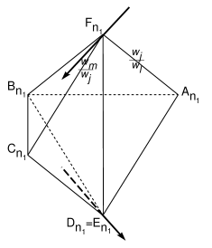
Now we assume the edge AB is collapsed to a point (see Figure 21). Then we obtain the following relations.
| (56) |
The identity (5.1) and the relation (56) can be obtained from (5.1) and (31) by sending and using the following property
The identities (5.1), (5.1) and (5.1) can be obtained from (5.1), (5.1) and (5.1) by sending , and , respectively.
∎
Proof of Theorem 1.3.
Now we prove the theorem by calculating the potential functions on each crossing . First, consider the case in which no edge of the octahedron on the positive crossing is collapsed. Let the variables assigned to the contributing sides be as in Figure 9 and let , , , as in Figure 10(a). Then the Yokota potential function of the crossing becomes
and
Likewise, let the variables assigned to the regions be as in Figure 9 and let , , , , as in Figure 10(a). Then the potential function of the colored Jones polynomial of the crossing becomes , which was defined in Lemma 3.1 for , and
We define the remaining term by the difference of two potential functions of the crossing . In this case, .
Assume satisfy the assumption of Lemma 5.1.121212 Any essential solution of and the corresponding essential solution of satisfy this assumption. Let
Then by (31),
and , . Applying these and (5.1) to (5) and (5), we obtain the remaining term of the crossing as follows.
By the same method, we can prove that the remaining term of the negative crossing in Figure 9 is the same as that of the positive crossing.
Now we consider the case in which only one horizontal edge is collapsed in an octahedron on a positive crossing . Let the region assigned to be the unbounded region and in Figure 9. Also let , , and , . Then the Yokota potential function of the crossing becomes
and
The potential function of the colored Jones polynomial of the crossing becomes
and
In this case, the remaining term is . Let
Then by (56),
and . Applying these and (5.1) to (5) and (5), we obtain the remaining term as follows.
By the same method, we can prove the remaining term of the negative crossing in this case is the same as that of the positive crossing. On the other hand, the remaining term becomes
when the region assigned to is the unbounded region,
when the region assigned to is the unbounded region, and
when the region assigned to is the unbounded region.
Now we consider the case when the crossing point is the endpoint of or . There are four cases as in Figure 22. We only prove the case of Figure 22(a) because the others can be proved by the same method.
First, we assume all three regions in Figure 22(a) are bounded. Then in Figure 10(a), the edge is collapsed to a point and , , , are assigned to the edges , , , , respectively. Also, we obtain
| (67) |
Applying (67) to Yokota potential function , we obtain
Also, applying (67) to the potential function of the colored Jones polynomial , we obtain
Using the well-known identity for from [6], we obtain the remaining term
Finally, we consider the case when the region assigned with in Figure 22(a) is unbounded. Then the edges and are collapsed to points. Furthermore, and , and , are assigned to the edges , in Figure 10(a), respectively. Applying
to Yokota potential function , we obtain
and to the potential function of the colored Jones polynomial , we obtain
Therefore, we obtain the remaining term
Likewise, we can show the remaining term becomes
when the region assigned to in Figure 22(a) is unbounded. The remaining three cases in Figure 22 can be obtained by the same method.
We complete the proof by proving
Note that we defined a contributing side of in Section 3.1. Assume the side assigned by in Figure 23 is a contributing side of . (This means that .)
If the side goes out of the crossing point , then the coefficient of in is , and if the side goes into the crossing point , then the coefficient of in is . They are cancelled by each other, and this happens for all the contributing sides.
∎
Appendix A Appendix
A.1 Formal substitution of the colored Jones polynomial and the potential function
In this Appendix, we induce the potential function defined in Section 3.2 from the formal substitution (1) of the colored Jones polynomial.
The colored Jones polynomial is determined by the R-matrix and the local maxima/minima (see [8] for reference). However, as seen in (1), the local maxima/minima do not have an effect on the formal substitution. So we only consider the R-matrix of the colored Jones polynomial:
where and is the Kronecker’s delta. If , then is uniquely determined by the formula , and if , then .
Note that this R-matrix is the inverse of the one in [8]. This implies the colored Jones polynomial of a knot here is the one of the mirror image in [8]. This choice is natural to [17] and Theorem 1.3.
Let be the hyperbolic knot with a fixed diagram and be the diagram defined in Section 2.1 with the orientation from to . We assign 0 to one bounded region of , then assign variables to the remaining bounded regions of and to the unbounded region. We assign variables to each side according to the signed sum of variables of adjacent regions with orientations modulo (see Figure 24 for an example).
For each non-trivalent vertex of , we assign the R-matrix to the positive crossing and the inverse to the negative crossing. Then we apply the formal substitution (1) to each R-matrix and substitute to as below. In the substitution process, if , then we put . Note that we apply the same R-matrix or its inverse in different forms according to the position of the collapsed horizontal edge. If none of the horizontal edges are collapsed in the octahedron, then we choose any formal substitution among the four possibilities. For positive crossings :
For negative crossings :
For the trivalent vertices of , we assign to the sides in or , then apply the same formal substitution to the R-matrix as follows (here, we use the same form of the R-matrix disregarding whether certain horizontal edge is collapsed or not).
For the endpoint of :
For the endpoint of :
Note that the colored Jones polynomial is expressed by the products of various forms of the R-matrices of crossings or trivalent vertices of (with slight modification by the local maxima/minima) and summed over all the possible indices (see [8] for the calculation of the colored Jones polynomial; the description in [8] may look slightly different from ours, but removing the sides of the tangle diagram assigned with 0 in [8] gives the diagram ). Now we define a potential function of the knot diagram by letting the product of all formal substitutions of to be . One important property of is that the variable assigned to the unbounded region appears only in the numerator. Therefore, we can define another potential function ,131313Note that . which coincides with the potential function defined in Section 3.2.
For example, and of Figure 24 become
and
This potential function coincides with the one defined previously in (5).
Note that using instead of does not violate the formulation of the optimistic limit because, for a solution of , becomes a solution of . We are considering only the solutions of with the condition because this condition corresponds to the collapsing process of tetrahedra of Thurston triangulation in Section 2.2 and the solutions correspond to the triangulation. However, other solutions with the condition also have good geometric meanings and this will be discussed in later papers.
A.2 Inessential solutions induced by essential solutions
Let and be the solutions in Lemma 1.2. In this Appendix, we determine the condition when an essential solution induces an inessential solution. Note that solutions and uniquely determine shape parameters of ideal tetrahedra in Yokota triangulation and in Thurston triangulation, respectively, and that, by definition, essential solution determines the shape parameters with none of them belonging to . Therefore, we focus on the shape parameters of each triangulation. We call the set of shape parameters of ideal tetrahedra essential when no elements of it belongs to .
Note that the shape parameters of two triangulations are determined by the local picture at each crossings and that, from Observation 2.1, what we have to consider are 3-2 moves and 4-5 moves at the crossings. Consider the two cases of Figure 20 and Figure 21, which correspond to 4-5 move and 3-2 move, respectively, and for which we have the determining relations of shape parameters in (31) and in (56), respectively.
Lemma A.1.
Proof.
From the relations (56) and (31), if one of the sets and is essential, then the shape parameters of the other set are expressed by products of nonzero and non-infinity numbers. This implies any shape parameter in the other set cannot be zero nor infinity. Therefore, what we have to check is the case when or for some .
Consider Figure 21. Assume is essential and . Then from , we obtain . Using , this induces , which contradicts the essentiality of . The case when is the same.
Conversely, assume is essential. By direct calculation from (56), we obtain
Now consider Figure 20. Assume is essential. Then direct calculation from (31) shows (69) is equivalent to
For example, using , we have
∎
From the above, if the essential solution in Lemma 1.2 determines the shape parameters of Yokota triangulation that satisfy the conditions (69) in Lemma A.1, then the corresponding solution is also essential. Conversely, the essential solution in Lemma 1.2 determines the shape parameters of Thurston triangulation that satisfy the conditions (68) and (74) in Lemma A.1, then the corresponding solution is also essential. We expect these conditions hold for almost all cases. For example, the essential solutions and of twist knots in [3] and [2], and the geometric solutions of the two-bridge knots in [13] satisfy these conditions. Furthermore, if every octahedron in the Yokota triangulation have one collapsed horizontal edge, then the essential solution always satisfies the condition. Therefore, essential solutions coming from the standard diagrams of 2-bridge knots in [13] always induce the essential solutions .
Acknowledgments The authors show gratitude to Yoshiyuki Yokota for sending us his preprint in advance before publication. This work was started when the first author was visiting Waseda university with Grant-in-Aid for JSPS Fellows 21.09221 and he is POSCO TJ Park fellow now. The first author was supported by Korea Research Foundation Grant funded by the Korean Government (KRF-2008-341-C00004) and the second author was supported by Grant-in-Aid for Scientific Research no. 22540236.
References
- [1] J. Cho. Yokota theory, the invariant trace fields of hyperbolic knots and the Borel regulator map. http://arxiv.org/abs/1005.3094, 2010.
- [2] J. Cho and J. Murakami. The complex volumes of twist knots via colored Jones polynomials. J. Knot Theory Ramifications, 19(11):1401–1421, 2010.
- [3] J. Cho, J. Murakami, and Y. Yokota. The complex volumes of twist knots. Proc. Amer. Math. Soc., 137(10):3533–3541, 2009.
- [4] S. Francaviglia. Hyperbolic volume of representations of fundamental groups of cusped 3-manifolds. Int. Math. Res. Not., (9):425–459, 2004.
- [5] R. M. Kashaev. The hyperbolic volume of knots from the quantum dilogarithm. Lett. Math. Phys., 39(3):269–275, 1997.
- [6] L. Lewin, editor. Structural properties of polylogarithms, volume 37 of Mathematical Surveys and Monographs. American Mathematical Society, Providence, RI, 1991.
- [7] R. Meyerhoff. Density of the Chern-Simons invariant for hyperbolic -manifolds. In Low-dimensional topology and Kleinian groups (Coventry/Durham, 1984), volume 112 of London Math. Soc. Lecture Note Ser., pages 217–239. Cambridge Univ. Press, Cambridge, 1986.
- [8] H. Murakami. The asymptotic behavior of the colored Jones function of a knot and its volume. Proceedings of ‘Art of Low Dimensional Topology VI’, edited by T. Kohno, January, 2000.
- [9] H. Murakami. Optimistic calculations about the Witten-Reshetikhin-Turaev invariants of closed three-manifolds obtained from the figure-eight knot by integral Dehn surgeries. Sūrikaisekikenkyūsho Kōkyūroku, (1172):70–79, 2000. Recent progress towards the volume conjecture (Japanese) (Kyoto, 2000).
- [10] H. Murakami. Kashaev’s invariant and the volume of a hyperbolic knot after Y. Yokota. In Physics and combinatorics 1999 (Nagoya), pages 244–272. World Sci. Publ., River Edge, NJ, 2001.
- [11] H. Murakami and J. Murakami. The colored Jones polynomials and the simplicial volume of a knot. Acta Math., 186(1):85–104, 2001.
- [12] H. Murakami, J. Murakami, M. Okamoto, T. Takata, and Y. Yokota. Kashaev’s conjecture and the Chern-Simons invariants of knots and links. Experiment. Math., 11(3):427–435, 2002.
- [13] K. Ohnuki. The colored Jones polynomials of 2-bridge link and hyperbolicity equations of its complements. J. Knot Theory Ramifications, 14(6):751–771, 2005.
- [14] D. Thurston. Hyperbolic volume and the Jones polynomial. Lecture note at “Invariants des noeuds et de variétés de dimension 3”, available at http://www.math.columbia.edu/~dpt/speaking/Grenoble.pdf, June 1999.
- [15] W. Thurston. The geometry and topology of three-manifolds. Lecture Note. available at http://www.msri.org/publications/books/gt3m/.
- [16] S. Tillmann. Degenerations of ideal hyperbolic triangulations. http://arxiv.org/abs/math/0508295.
- [17] Y. Yokota. On the volume conjecture for hyperbolic knots. http://arxiv.org/abs/math/0009165.
- [18] Y. Yokota. On the complex volume of hyperbolic knots. J. Knot Theory Ramifications, 20(7):955–976, 2011.
- [19] C. K. Zickert. The volume and Chern-Simons invariant of a representation. Duke Math. J., 150(3):489–532, 2009.
School of Mathematics, Korea Institute for Advanced Study, 85 Hoegiro, Dongdaemun-gu, Seoul 130-722, Republic of Korea
Department of Mathematics, Faculty of Science and Engineering, Waseda University, 3-4-1 Okubo, Shinjuku-ku, Tokyo 169-8555, Japan
E-mail: dol0425@gmail.com
murakami@waseda.jp