A Unified View of Regularized Dual Averaging
and Mirror Descent with Implicit Updates

Abstract

We study three families of online convex optimization algorithms: follow-the-proximally-regularized-leader (FTRL-Proximal), regularized dual averaging (RDA), and composite-objective mirror descent. We first prove equivalence theorems that show all of these algorithms are instantiations of a general FTRL update. This provides theoretical insight on previous experimental observations. In particular, even though the FOBOS composite mirror descent algorithm handles $L_{1}$ regularization explicitly, it has been observed that RDA is even more effective at producing sparsity. Our results demonstrate that FOBOS uses subgradient approximations to the $L_{1}$ penalty from previous rounds, leading to less sparsity than RDA, which handles the cumulative penalty in closed form. The FTRL-Proximal algorithm can be seen as a hybrid of these two, and outperforms both on a large, real-world dataset.

Our second contribution is a unified analysis which produces regret bounds that match (up to logarithmic terms) or improve the best previously known bounds. This analysis also extends these algorithms in two important ways: we support a more general type of composite objective and we analyze implicit updates, which replace the subgradient approximation of the current loss function with an exact optimization.

Keywords: online learning, online convex optimization, subgradient methods, regret bounds, follow-the-leader algorithms

1 Introduction

We consider the problem of online convex optimization, and in particular its application to online learning. On each round $t=1,\dots,T$, we must pick a point $x_{t}\in\mathbb{R}^{n}$. A convex loss function $f_{t}$ is then revealed, and we incur loss $f_{t}(x_{t})$. Our regret at the end of $T$ rounds with respect to a comparator point $\mathring{x}$ is

$$\text{Regret}\equiv\sum_{t=1}^{T}f_{t}(x_{t})-\sum_{t=1}^{T}f_{t}(\mathring{x}).$$

In Section 4 we provide a unified regret analysis of three prominent algorithms for online convex optimization. In recent years, these algorithms have received significant attention because they have straightforward and efficient implementations and offer state-of-the-art performance for many large-scale applications. In particular, we consider:

• Follow-the-Proximally-Regularized-Leader (FTPRL), introduced with adaptive learning rates (regularization) by McMahan and Streeter (2010).

• Regularized Dual Averaging (RDA), introduced by Xiao (2009) and extended with adaptive learning rates by Duchi et al. (2010a).

• Composite-Objective Mirror Descent (COMID) algorithms Duchi et al. (2010b), including FOBOS Duchi and Singer (2009).

As pointed out by Duchi et al. (2010b), the analyses of RDA and COMID cited above are completely different. In contrast, we provide a unified analysis of these algorithms. One of our contributions is simply demonstrating that this large and important family of algorithms can be analyzed using a common argument, but our analysis also generalizes previous results in several important ways. First, we extend all of these algorithm to handle implicit updates, which replace the first-order approximation on the current loss function with an exact optimization. In many practical situations this update can be solved efficiently, and offers both theoretical and practical benefits compared to the first-order update.

We also extend the ability of these algorithms to handle composite objectives (objectives that include a fixed non-smooth term $\Psi$). Previous work considers loss functions on each round of the form $f_{t}(x)+\Psi(x)$, where $f_{t}$ is approximated by a linear function, but the optimization over $\Psi$ is exact. However, as discussed below, continuing to add a new copy of $\Psi(x)$ on each round may be undesirable in some cases; to address this, we analyze loss functions of the form $f_{t}(x)+\alpha_{t}\Psi(x)$ where $\alpha_{t}$ is a non-increasing sequence of non-negative numbers. This is useful, for example, if one wishes to encode a Bayesian prior in the online setting (see Section 2.2). Our proof technique has the advantage that handling this general form of composite updates requires only a few extra lines beyond the non-composite proof. The original analysis of FTPRL by McMahan and Streeter (2010) did not support composite updates. In addition to remedying this, we prove a new stronger version of the “FTRL/BTL Lemma” which tightens the analysis of FTPRL by a constant factor. The new lemma is quite general and may be of independent interest.

Our unified analysis relies on a formulation of all of these algorithms as instances of follow-the-regularized-leader, which we develop in Section 3. A preliminary version of these equivalence results appeared in McMahan (2010). Our equivalence theorems apply to algorithms that use arbitrary strongly convex regularization; however, these results show that the most interesting strict equivalences occur in the case of quadratic regularization. Thus, for the analysis of Section 4 we restrict attention to this case, namely to algorithms where the incremental strong convexity is of the form

$$R_{t}(x)=\frac{1}{2}\big{\|}Q_{t}^{\frac{1}{2}}(x-y)\big{\|}^{2}_{2}$$

where $y\in R^{n}$ and $Q_{t}$ is a positive-semidefinite matrix. This is less general than previous results in terms of arbitrary strongly-convex functions or Bregman divergences.

Application to Sparse Models via $L_{1}$ Regularization

On the surface, follow-the-regularized-leader algorithms like regularized dual averaging Xiao (2009) appear quite different from gradient descent (and more generally, mirror descent) style algorithms like FOBOS Duchi and Singer (2009). However, the results of Section 3 show that in the case of quadratic stabilizing regularization there are only two differences between the algorithms:

• How they choose to center the additional strong convexity used to guarantee low regret: RDA centers this regularization at the origin, while FOBOS centers it at the current feasible point.

• How they handle an arbitrary non-smooth regularization function $\Psi$. This includes the mechanism of projection onto a feasible set and how $L_{1}$ regularization is handled.

To make these differences precise while also illustrating that these families are actually closely related, we consider a third algorithm, FTRL-Proximal. When the non-smooth term $\Psi$ is omitted, this algorithm is in fact identical to FOBOS. On the other hand, its update is essentially the same as that of dual averaging, except that additional strong convexity is centered at the current feasible point (see Table 1).

Previous work has shown experimentally that dual averaging with $L_{1}$ regularization is much more effective at introducing sparsity than FOBOS Xiao (2009), Duchi et al. (2010a). Our equivalence theorems provide a theoretical explanation for this: while RDA considers the cumulative $L_{1}$ penalty $t\lambda\|x\|_{1}$ on round $t$, FOBOS (when viewed as a global optimization using our equivalence theorem) considers $\phi_{1:t-1}\cdot x+\lambda\|x\|_{1}$, where $\phi_{s}$ is a certain subgradient approximation of $\lambda\|x_{s}\|_{1}$ (we use $\phi_{1:t-1}$ as shorthand for $\sum_{s=1}^{t-1}\phi_{s}$, and extend the notation to sums over matrices and functions as needed).

An experimental comparison of FOBOS, RDA, and FTRL-Proximal, presented in Section 5, demonstrates the validity of the above explanation. The FTRL-Proximal algorithm behaves very similarly to RDA in terms of sparsity, confirming that it is the cumulative subgradient approximation to the $L_{1}$ penalty that causes decreased sparsity in FOBOS.

In recent years, online gradient descent and stochastic gradient descent (its batch analogue) have proven themselves to be excellent algorithms for large-scale machine learning. In the simplest case FTRL-Proximal is identical, but when $L_{1}$ or other non-smooth regularization is needed, FTRL-Proximal significantly outperforms FOBOS, and can outperform RDA as well. Since the implementations of FTRL-Proximal and RDA only differ by a few lines of code, we recommend trying both and picking the one with the best performance in practice.

$$\begin{array}[]{rcc*{3}{l@{\qquad}}}&&\ (A)&\qquad(B)&\qquad(C)\\ \vspace{2pt}\text{COMID}&\mathop{\rm arg\,min}_{x}&g^{\prime}_{1:t-1}\cdot x+f_{t}(x)&+\ \ \phi_{1:t-1}\cdot x+\alpha_{t}\Psi(x)&+\frac{1}{2}\sum_{s=1}^{t}\|Q_{s}^{\frac{1}{2}}(x-x_{s})\|^{2}\\ \vspace{2pt}\text{RDA}&\mathop{\rm arg\,min}_{x}&g^{\prime}_{1:t-1}\cdot x+f_{t}(x)&+\ \ \alpha_{1:t}\Psi(x)&+\frac{1}{2}\sum_{s=1}^{t}\|Q_{s}^{\frac{1}{2}}(x-0)\|^{2}\\ \text{FTPRL}&\mathop{\rm arg\,min}_{x}&g^{\prime}_{1:t-1}\cdot x+f_{t}(x)&+\ \ \alpha_{1:t}\Psi(x)&+\frac{1}{2}\sum_{s=1}^{t}\|Q_{s}^{\frac{1}{2}}(x-x_{s})\|^{2}\\ \text{AOGD}&\mathop{\rm arg\,min}_{x}&g^{\prime}_{1:t-1}\cdot x+f_{t}(x)&+\ \ \phi_{1:t-1}\cdot x+\Psi(x)&+\frac{1}{2}\sum_{s=1}^{t}\|Q_{s}^{\frac{1}{2}}(x-0)\|^{2}_{2}\\ \end{array}$$

Table 1: The algorithms considered in this paper, expressed as particular instances of the update of Eq. (3). The fact that we can express COMID and adaptive online gradient descent (AOGD) in this way is a consequence of Theorems 4 and 7. Each algorithms’ objective has three components: (A) An approximation to the sum of previous loss functions $f_{1:t}$, where the first $t-1$ functions are approximated by linear terms, and $f_{t}$ is included exactly (exactly including $f_{t}$ make the updates implicit). (B) Terms for the non-smooth composite terms $\alpha_{t}\Psi$. COMID approximates the terms for $\alpha_{1:t-1}\Psi$ by subgradients, while RDA and FTPRL consider them exactly. And finally, (C), stabilizing regularization needed to ensure low regret.

2 Algorithms and Regret Bounds

We begin by establishing notation and introducing more formally the algorithms we consider. We consider loss functions $f_{t}(x)+\alpha_{t}\Psi(x)$, where $\Psi$ is a fixed (typically non-smooth) regularization function. In a typical online learning setting, given an example $(\theta_{t},y_{t})$ where $\theta_{t}\in\mathbb{R}^{n}$ is a feature vector and $y_{t}\in\{-1,1\}$ is a label, we take $f_{t}(x)=\text{loss}(\theta_{t}\cdot x,y_{t})$. For example, for logistic regression we use log-loss, $\text{loss}(\theta_{t}\cdot x,y_{t})=\log(1+\exp(-y_{t}\theta_{t}\cdot x)).$ All of the algorithms we consider support composite updates (consideration of $\Psi$ explicitly rather than through a gradient $\triangledown f_{t}(x_{t})$) as well as positive semi-definite matrix learning rates $Q$ which can be chosen adaptively (the interpretation of these matrices as learning rates will be clarified in Section 3).

We first consider the specific algorithms used in the $L_{1}$ experiments of Section 5; we use the standard reduction to linear functions, letting $g_{t}=\triangledown f_{t}(x_{t})$. The first algorithm we consider is from the gradient-descent family, namely FOBOS, which plays

$$x_{t+1}=\mathop{\rm arg\,min}_{x}g_{t}\cdot x+\lambda\big{\|}x\big{\|}_{1}+\frac{1}{2}\big{\|}Q_{1:t}^{\frac{1}{2}}(x-x_{t})\big{\|}^{2}_{2}.$$

We state this algorithm implicitly as an optimization, but a gradient-descent style closed-form update can also be given (Duchi and Singer, 2009). The algorithm was described in this form as a specific composite-objective mirror descent (COMID) algorithm by Duchi et al. (2010b).

The regularized dual averaging (RDA) algorithm of Xiao (2009) plays

$$x_{t+1}=\mathop{\rm arg\,min}_{x}g_{1:t}\cdot x+t\lambda\big{\|}x\big{\|}_{1}+\frac{1}{2}\sum_{s=1}^{t}\big{\|}Q_{s}^{\frac{1}{2}}(x-0)\big{\|}^{2}_{2}.$$

In contrast to FOBOS, the RDA optimization is over the sum $g_{1:t}$ rather than just the most recent gradient $g_{t}$. We will show (in Theorem 7) that when $\lambda=0$ and the $f_{t}$ are not strongly convex, this algorithm is in fact equivalent to the adaptive online gradient descent (AOGD) algorithm of  Bartlett et al. (2007).

RDA is directly defined as a FTRL algorithm, and hence is also an instance of the more general primal-dual algorithmic schema of Shalev-Shwartz and Singer (2006); see also Kakade et al. (2009). However, these general results are not sufficient to prove the original bounds for RDA, nor the versions here that extend to implicit updates.

The FTRL-Proximal algorithm plays

$$x_{t+1}=\mathop{\rm arg\,min}_{x}g_{1:t}\cdot x+t\lambda\big{\|}x\big{\|}_{1}+\frac{1}{2}\sum_{s=1}^{t}\big{\|}Q_{s}^{\frac{1}{2}}(x-x_{s})\big{\|}^{2}_{2}.$$

This algorithm was introduced by McMahan and Streeter (2010), but without support for an explicit $\Psi$.

One of our principle contributions is showing the close connection between all four of these algorithms; Table 1 summarizes the key results from Theorems 4 and 7, writing AOGD and FOBOS in a form that makes the relationship to RDA and FTRL-Proximal explicit.

In our equivalence analysis, we will consider arbitrary convex functions $R_{t}$ and $\tilde{R}_{t}$ in place of the $\frac{1}{2}\big{\|}Q_{t}^{\frac{1}{2}}x\big{\|}_{2}^{2}$ and $\frac{1}{2}\big{\|}Q_{t}^{\frac{1}{2}}(x-x_{t})\big{\|}^{2}_{2}$ that appear here, as well as arbitrary convex $\Psi(x)$ in place of $\lambda\|x\|_{1}$.

2.1 Implicit and Composite Updates for FTRL

The algorithms we consider can be expressed as follow-the-regularized-leader (FTRL) algorithms that perform implicit and composite updates. The standard subgradient FTRL algorithm uses the update

$$x_{t+1}=\mathop{\rm arg\,min}_{x}\left(\sum_{s=1}^{t}\triangledown f_{s}(x_{s})\right)\cdot x+R_{1:t}(x).$$

In this update, each previous (potentially non-linear) loss function $f_{s}$ is approximated by the gradient at $x_{s}$ (when $f_{s}$ is not differentiable, we can use a subgradient at $x_{s}$ in place of the gradient). The functions $R_{t}$ are incremental regularization added on each round; for example $R_{1:t}(x)=\sqrt{t}\|x\|^{2}$ is a standard choice, corresponding to regularized dual averaging.

Implicit update rules are usually defined for mirror descent algorithms, but we can define an analogous update for FTRL:

$$x_{t+1}=\mathop{\rm arg\,min}_{x}\left(\sum_{s=1}^{t-1}\triangledown f_{s}(x_{s+1})\right)\cdot x+f_{t}(x)+R_{1:t}(x).$$

This update replaces the subgradient approximation of $f_{t}$ with the possibly non-linear $f_{t}$. Closed-form implicit updates for the squared error case were derived by Kivinen and Warmuth (1997); the term implicit updates was coined later Kivinen et al. (2006). Our formulation is similar to the online coordinate-dual-ascent algorithm briefly mentioned by Shalev-Shwartz and Kakade (2008). In general, computing the implicit update might require solving an arbitrary convex optimization problem (hence, the name implicit), however, in many useful applications it can be computed in closed form or by optimizing a one-dimensional problem. We discuss the advantages of implicit updates in Section 2.2.

Analysis of implicit updates has proved difficult. Kulis and Bartlett (2010) provide the only other regret bounds for implicit updates that match those of the explicit-update versions. While their analysis handles more general divergences, it only applies to mirror-descent algorithms. Our analysis handles composite objectives and applies FTRL algorithms as well as mirror descent. Our analysis also quantifies the one-step improvement in the regret bound obtained by the implicit update, showing the inequality is in fact strict when the implicit update is non-trivial.

When $f_{t}$ is not differentiable, we use the update

$$x_{t+1}=\mathop{\rm arg\,min}_{x}g^{\prime}_{1:t-1}\cdot x+f_{t}(x)+R_{1:t}(x),$$ (1)

where $g^{\prime}_{t}$ is a subgradient of $f_{t}$ at $x_{t+1}$ (that is, $g^{\prime}_{t}\in\partial f_{t}(x_{t+1})$) such that $g^{\prime}_{1:t-1}+g_{t}^{\prime}+\triangledown R_{1:t}(x_{t+1})=0.$ The existence of such a subgradient is proved below, in Theorem 3.

In many applications, we have a fixed convex function $\Psi$ that we also wish to include in the optimization, for example $\Psi(x)=\|x\|_{1}$ ($L_{1}$-regularization to induce sparsity) or the indicator function on a feasible set $\mathcal{F}$ (see Section 2.4). While it is possible to approximate this function via subgradients as well, when computationally feasible it is often better to handle $\Psi$ directly. For example, in the case where $\Psi(x)=\|x\|_{1}$, subgradient approximations will in general not lead to sparse solutions. In this case, closed-form updates for optimizations including $\Psi$ are often possible, and produce much better sparsity Xiao (2009), Duchi and Singer (2009). We can include such a term directly in FTRL, giving the composite objective update

$$x_{t+1}=\mathop{\rm arg\,min}_{x}\left(\sum_{s=1}^{t}\triangledown f_{s}(x_{s})\right)\cdot x+\alpha_{1:t}\Psi(x)+R_{1:t}(x),$$ (2)

where $\alpha_{t}$ is the weight on $\Psi$ on round $t$.

This formulation, which allows for an arbitrary sequence of non-negative, non-increasing $\alpha_{t}$’s, is more general than that supported by the original analysis of COMID or RDA. Xiao (2010, Sec 6.1) shows that RDA does allow a varying schedule where $\alpha_{1:t}=c+1/\sqrt{t}$ for a constant $c$, by incorporating part of the $\Psi$ term in the regularization function $R_{t}$; this is less general than our analysis, which allows the schedule $\alpha_{t}$ to be chosen independently of the learning rate.

Finally, we can combine these ideas to define an implicit update with a composite objective. In the general case where $f_{t}$ is not differentiable, we have the update

$$x_{t+1}=\mathop{\rm arg\,min}_{x}g^{\prime}_{1:t-1}\cdot x+f_{t}(x)+\alpha_{1:t}\Psi(x)+R_{1:t}(x),$$ (3)

where $g^{\prime}_{t}\in\partial f_{t}(x_{t+1})$ such that $\exists\phi_{t}\in\partial\Psi(x_{t+1})$ where $g^{\prime}_{1:t-1}+g^{\prime}_{t}+\phi_{t}+\triangledown R_{1:t}(x_{t+1})=0.$ The existence of such a subgradient again follows from Theorem 3.

It is worth noting that our analysis of implicit updates applies immediately to standard first-order updates. Let $f^{w}_{t}$ designate the loss function provided by the world, and let $f^{u}_{t}$ be the loss function in the update Eq. (3). Then we recover the non-implicit algorithms by taking $f^{u}_{t}(x)\leftarrow\triangledown f^{w}_{t}(x_{t})\cdot x$.

2.2 Motivation for Implicit Updates and Composite Objectives

Implicit updates offer a number of advantages over using a subgradient approximation. Kulis and Bartlett (2010) discusses several important examples. They also observe that empirically, implicit updates outperform or nearly outperform linearized updates, and show more robustness to scaling of the data.

Learning problems that use importance weights on examples are also a good candidate for implicit updates. Importance weights can be used to compress the training data, by replacing $n$ copies of an example with one copy with weight $n$. They also arise in active learning algorithms Beygelzimer et al. (2010) and situations where the training and test distributions differ (covariate shift, e.g. Sugiyama et al. (2008)). Recent work has demonstrated experimentally that implicit updates can significantly outperform first-order updates both on importance weighted and standard learning problems Karampatziakis and Langford (2010).

The following simple examples demonstrates the intuition for these improvements. The key is that the linearization of $f_{t}$ over-estimates the decrease in loss under $f_{t}$ achieved by moving in the direction $\triangledown f_{t}(x_{t})$. The farther $x_{t+1}$ is chosen from $x_{t}$, and the more non-linear the $f_{t}$, the worse this approximation can be. Consider gradient descent in one dimension with $f_{t}(x)=\frac{1}{2}(x-3)^{2}$ and $x_{t}=2$. Then $\triangledown f_{t}(2)=-1$, and if we choose a learning rate $\eta_{t}>1$, we will actually overshoot the optimum for $f_{t}$ (such a learning rate could be indicated by the theory if the feasible set is large, for example). Implicit updates, on the other hand, will never choose $x_{t+1}>3$, rather $x_{t+1}\rightarrow 3$ as $\eta_{t}\rightarrow\infty$. Thus, we see implicit updates can be significantly better behaved with large learning rates. Note that an importance weight of $n$ is equivalent to multiplying the learning rate by $n$, so when importance weights can be large, implicit updates can be particularly beneficial.

The overshooting issue is even more pronounced with non-smooth objectives, for example, $f_{t}(x)=g\cdot x+\|x\|_{1}$. A standard gradient descent update will in general never set $x_{t+1}=0$ despite the $L_{1}$ regularization; handling the $L_{1}$ term via an implicit update solves this problem. This is exactly the insight that COMID algorithms like FOBOS exploit; by analyzing general implicit updates, we achieve an analysis of these algorithms while also supporting a much larger class of updates.

When the functional form of the non-smooth component of the objective (for example $\|x\|_{1}$) is fixed across rounds, it is preferable to perform an explicit optimization involving the total non-smooth contribution $\alpha_{1:t}\Psi$ (RDA and FTPRL) rather than just the round $t$ contribution $\alpha_{t}\Psi$ (COMID). While RDA supports this type of non-smooth objective, it requires the weight on $\Psi$ to be fixed across rounds. We generalize this to non-increasing per-round contributions in this work.

Suppose one is performing online logistic regression, and believes a priori that the coefficients have a Laplacian distribution. Then, $L_{1}$-penalized logistic regression corresponds to MAP estimation (e.g., Lee et al. (2006)); suppose the prior corresponds to a total penalty of $\lambda\|x\|_{1}$. If the size of the dataset $T$ is known in advance, then we can use $\alpha_{t}=\lambda/T$, and by making multiple passes over the data, we will converge to the MAP estimate. However, in the online setting we will in general not know $T$ in advance, and we may wish to use an online algorithm for computational efficiency. In this case, any fixed value of $\alpha_{t}$ will correspond to strengthening the prior each time we see a new example, which is undesirable. With the generalized notion of composite updates introduced here, this problem is overcome by choosing $\alpha_{1}\Psi(x)=\lambda\|x\|_{1}$, and $\alpha_{t}=0$ for $t\geq 2$. Thus, the fixed penalty on the coefficients is correctly encoded, independent of $T$.

2.3 Summary of Regret Bounds

In Section 4, we analyze the update rule of Equation (3) when

$$R_{t}(x)=\frac{1}{2}\big{\|}Q_{t}^{\frac{1}{2}}(x-y_{t})\big{\|}^{2},$$ (4)

where $\|\cdot\|=\|\cdot\|_{2}$ here and throughout. The points $y_{t}\in\mathbb{R}^{n}$ are the centers for the additional regularization added on each round. Choosing $y_{t}=0$ leads to an analysis of RDA with implicit updates, and choosing $y_{t}=x_{t}$ yields the follow-the-proximally-regularized-leader algorithm with implicit updates. Using $y_{t}=x_{t}$ together with a modified choice of $f_{t}$ leads to composite-objective mirror descent (see Section 3).

The generalized learning rates $Q_{t}$ can be chosen adaptively using techniques from McMahan and Streeter (2010) and Duchi et al. (2010a), which leads to improved regret bounds, as well as algorithms that perform much better in practice Streeter and McMahan (2010). Since in this work we provide suitable regret bounds in terms of arbitrary $Q_{t}$, the adaptive techniques can be applied directly. Doing so complicates the exposition somewhat, and so for simplicity and easy of comparison to previous results we state specific regret bounds for scalar learning rates:

Corollary 1.

Let $\Psi$ be the indicator function on a feasible set $\mathcal{F}$, and let $D=\max_{a,b\in\mathcal{F}}\|a-b\|$. So that our bounds are comparable, suppose $\max_{a\in\mathcal{F}}\|a\|=\frac{D}{2}$ (for example, if $\mathcal{F}$ is symmetric). Let $f_{t}$ be a sequence of convex loss functions such that $\|\triangledown f_{t}(x)\|\leq G$ for all $t$ and all $x\in\mathcal{F}$. Then for FTPRL we set $x_{t}=y_{t}$ and have

$$\text{Regret}\leq DG\sqrt{2T}.$$

Implicit-update mirror descent obtains the same bound. For regularized dual averaging we choose $y_{t}=0$ for all $t$, and obtain

$$\text{Regret}\leq\frac{1}{2}DG\sqrt{2T}+\frac{GD}{\sqrt{2}}\ln T+\mathcal{O}(1).$$

These bounds are achieved with an adaptive learning rate that depends only on $t$ ($T$ need not be known in advance). If $T$ is known, then the $\sqrt{2}$ constant on the $\sqrt{T}$ terms can be eliminated. The regret bounds with per-coordinate adaptive rates are at least as good, and often better. This corollary is a direct consequence of the following general result:

Theorem 2.

Let $\Psi$ be an extended convex function on $\mathbb{R}^{n}$ with $\Psi(x)\geq 0$ and $0\in\partial\Psi(0)$, let $f_{t}$ be a sequence of convex loss functions, and let $\alpha_{t}\in\mathbb{R}$ be non-negative and non-increasing real numbers ($0\leq\alpha_{t+1}\leq\alpha_{t}$). Consider the FTRL algorithm that plays $x_{1}=0$ and afterwards plays according to Equation (3),

$$x_{t+1}=\mathop{\rm arg\,min}_{x}g^{\prime}_{1:t-1}\cdot x+f_{t}(x)+\alpha_{1:t}\Psi(x)+R_{1:t}(x),$$

using incremental quadratic regularization functions $R_{t}(x)=\frac{1}{2}\big{\|}Q_{t}^{\frac{1}{2}}(x-y_{t})\big{\|}^{2}$ where $Q_{1}\in S^{n}_{++}$, $Q_{t}\in S^{n}_{+}$ for $t>1$, and $y_{t}\in\mathbb{R}^{n}$. Then there exist $\tilde{g}_{t}\in R^{n}$ such that

$$\text{Regret}(f) \leq R_{1:T}(\mathring{x})+\alpha_{1:T}\Psi(\mathring{x})+\sum_{t=1}^{T}(g_{t}-\frac{1}{2}\tilde{g}_{t})^{\top}Q_{1:t}^{-1}\tilde{g}_{t}-g_{t}Q_{1:t}^{-1}Q_{t}(y_{t}-x_{t})$$

$$\leq R_{1:T}(\mathring{x})+\alpha_{1:T}\Psi(\mathring{x})+\sum_{t=1}^{T}\frac{1}{2}\big{\|}Q_{1:t}^{-\frac{1}{2}}g_{t}\big{\|}^{2}-\delta_{1:t}-g_{t}Q_{1:t}^{-1}Q_{t}(y_{t}-x_{t})$$

versus any point $\mathring{x}\in\mathbb{R}^{n}$, for any $g_{t}\in\partial f_{t}(x_{t})$, with $\delta\geq 0$.

We will show that $\tilde{g}_{t}$ is a certain subgradient of $f_{t}$, and in fact when all $\alpha_{t}=0$, then $\tilde{g}_{t}\in\partial f_{t}(x_{t+1})$. If $f_{t}$ is strictly convex, then in general $\tilde{g}_{t}\neq g_{t}$, and so the inequality between the first and second bounds can be strict; in fact, we will show that on rounds $t$ where the implicit-update is non-trivial, $\delta>0$, indicating a one-step advantage for implicit updates. When all $\alpha_{t}=0$, $\delta_{t}$ is one-half the improvement in the objective function of Equation (3) obtained by solving for the optimum point rather than using a solution from the linearized problem; the proof of Lemma 11 makes this precise.

For RDA, we take $y_{t}=0$, and for FTPRL and implicit-update mirror descent we take $y_{t}=x_{t}$. Since no restrictions are placed on the $y_{t}$ in the theorem, the final right-hand term being subtracted could have be positive, negative, or zero.

If we treat $\alpha_{t}\Psi$ as an intrinsic part of the problem, that is, we are measuring loss against $f_{t}(x)+\alpha_{t}\Psi(x)$, then the $\alpha_{1:T}\Psi(\mathring{x})$ term disappears from the regret bound.

2.4 Notation and Technical Background

We use the notation $g_{1:t}$ as a shorthand for $\sum_{s=1}^{t}g_{s}$. Similarly we write $Q_{1:t}$ for a sum of matrices $Q_{t}$, and we use $f_{1:t}$ to denote the function $f_{1:t}(x)=\sum_{s=1}^{t}f_{s}(x)$. We assume the summation binds more tightly than exponents, so $Q_{1:t}^{\frac{1}{2}}=(Q_{1:t})^{\frac{1}{2}}$. We write $x^{\top}y$ or $x\cdot y$ for the inner product between $x,y\in\mathbb{R}^{n}$. We write “the functions $f_{t}$” for the sequence of functions $(f_{1},\dots,f_{T})$.

We write $S^{n}_{+}$ for the set of symmetric positive semidefinite $n\times n$ matrices, with $S^{n}_{++}$ the corresponding set of symmetric positive definite matrices. Recall $A\in S^{n}_{++}$ means $\forall x\neq 0,\ x^{\top}Ax>0$. Since $A\in S^{n}_{+}$ is symmetric, $x^{\top}Ay=y^{\top}Ax$ (we often use this result implicitly). For $B\in S^{n}_{+}$, we write $B^{1/2}$ for the square root of $B$, the unique $X\in S^{n}_{+}$ such that $XX=B$ (see, for example, Boyd and Vandenberghe (2004, A.5.2)).

Unless otherwise stated, convex functions are assumed to be extended, with domain $\mathbb{R}^{n}$ and range $\mathbb{R}\cup\left\{\infty\right\}$ (see, for example (Boyd and Vandenberghe, 2004, 3.1.2)). For a convex function $f$, we let $\partial f(x)$ denote the set of subgradients of $f$ at $x$ (the subdifferential of $f$ at $x$). By definition, $g\in\partial f(x)$ means $f(y)\geq f(x)+g^{\top}(y-x)$ for all $y$. When $f$ is differentiable, we write $\triangledown f(x)$ for the gradient of $f$ at $x$. In this case, $\partial f(x)=\left\{\triangledown f(x)\right\}$. All mins and argmins are over $\mathbb{R}^{n}$ unless otherwise noted. We make frequent use of the following standard results, summarized as follows:

Theorem 3.

Let $R:\mathbb{R}^{n}\rightarrow\mathbb{R}$ be strongly convex with continuous first partial derivatives, and let $\Phi$ and $f$ be arbitrary (extended) convex functions. Then,

1. Let $U(x)=R(x)+\Phi(x)$. Then, there exists a unique pair $(x^{*},\phi^{*})$ such that both

   $$\qquad\phi^{*}\in\partial\Phi(x^{*})\qquad\text{and}\qquad\qquad x^{*}=\mathop{\rm arg\,min}_{x}R(x)+\phi^{*}\cdot x.$$

   Further, this $x^{*}$ is the unique minimizer of $U$, and $\triangledown R(x^{*})+\phi^{*}=0$.

2. Let $V(x)=R(x)+\Phi(x)+f(x)$ and $\mathring{x}=\mathop{\rm arg\,min}_{x}V(x)$. Then, there exists a $g\in\partial f(\mathring{x})$ such that

   $$\mathring{x}=\mathop{\rm arg\,min}_{x}R(x)+\Phi(x)+g\cdot x.$$

Proof.

First we consider part $A$. Since $R$ is strongly convex, $U$ is strongly convex, and so has a unique minimizer $x^{*}$ (see for example, (Boyd and Vandenberghe, 2004, 9.1.2)). Let $r=\triangledown R$. Since $x^{*}$ is a minimizer of $U$, there must exist a $\phi^{*}\in\partial\Phi(x^{*})$ such that $r(x^{*})+\phi^{*}=0$, as this is a necessary (and sufficient) condition for $0\in\partial U(x^{*})$. It follows that $x^{*}=\mathop{\rm arg\,min}_{x}R(x)+\phi^{*}\cdot x$, as $r(x^{*})+\phi^{*}$ is the gradient of this objective at $x^{*}$. Suppose some other $(x^{\prime},\phi^{\prime})$ satisfies the conditions of the theorem. Then, $r(x^{\prime})+\phi^{\prime}=0$, and so $0\in\partial U(x^{\prime})$, and so $x^{\prime}$ is a minimizer of $U$. Since this minimizer is unique, $x^{\prime}=x^{*}$, and $\phi^{\prime}=-r(x^{*})=\phi^{*}$. An equivalent condition to $x^{*}=\mathop{\rm arg\,min}_{x}R(x)+\phi^{*}\cdot x$ is $\triangledown R(x^{*})+\phi^{*}=0$.

For part $B$, by definition of optimality, there exists a $\phi\in\partial\Phi(\mathring{x})$ and a $g\in\partial f(\mathring{x})$ such that $g+\phi+\triangledown R(\mathring{x})=0$. Choosing this $g$, define

$$\hat{x}=\mathop{\rm arg\,min}_{x}R(x)+\Phi(x)+g\cdot x.$$

Applying part $A$ with $R(x)\leftarrow R(x)+g\cdot x$, there exists a unique pair $(\hat{x},\hat{\phi})$ such that $\hat{\phi}\in\partial\Phi(\hat{x})$ and $\triangledown R(\hat{x})+\hat{\phi}+g=0$. Since $(\mathring{x},\phi)$ satisfy this equation, we conclude $\mathring{x}=\hat{x}$. ∎

Feasible Sets

In some applications, we may be restricted to only play points from a convex feasible set $\mathcal{F}\subseteq\mathbb{R}^{n}$, for example, the set of (fractional) paths between two nodes in a graph. A feasible set is also necessary to prove regret bounds against linear functions. With composite updates, Equations (2) and (3), this is accomplished for free by choosing $\Psi$ to be the indicator function $I_{\mathcal{F}}$ on $\mathcal{F}$, where $I_{\mathcal{F}}(x)=0$ for $x\in\mathcal{F}$ and $\infty$ otherwise. It is straightforward to verify that

$$\mathop{\rm arg\,min}_{x\in\mathbb{R}^{n}}g_{1:t}\cdot x+R_{1:t}(x)+I_{\mathcal{F}}(x)\quad=\quad\mathop{\rm arg\,min}_{x\in\mathcal{F}}g_{1:t}\cdot x+R_{1:t}(x),$$

and so in this work we can generalize (for example) the results of McMahan and Streeter (2010) for specific feasible sets without specifically discussing $\mathcal{F}$, and instead considering arbitrary extended convex functions $\Psi$. Note that in this case the choice of $\alpha_{t}$ does not matter as long as $\alpha_{1}>0$.

3 Mirror Descent Follows The Leader

In this section we consider the relationship between mirror descent algorithms (the simplest example being online gradient descent) and FTRL algorithms. Let $f_{t}(x)=g_{t}\cdot x+\Psi(x)$.

Let $R_{1}$ be strongly convex, with all the $R_{t}$ convex. We assume that $\min_{x}R_{1}(x)=0$, and assume that $x=0$ is the unique minimizer unless otherwise noted.

Follow The Regularized Leader (FTRL)

The simplest follow-the-regularized-leader algorithm plays

$$x_{t+1}=\mathop{\rm arg\,min}_{x}g_{1:t}\cdot x+\frac{\sigma_{1:t}}{2}\|x\|^{2}_{2},$$ (5)

where $\sigma_{1:t}\in\mathbb{R}$ is the amount of stabilizing strong convexity added.

A more general update is

$$x_{t+1}=\mathop{\rm arg\,min}_{x}g_{1:t}\cdot x+R_{1:t}(x).$$

where we add an additional convex function $R_{t}$ on each round. When $\mathop{\rm arg\,min}_{x\in\mathbb{R}^{n}}R_{t}(x)=0,$ we call the functions $R_{t}$ (and associated algorithms) origin-centered. We can also define proximal versions of FTRL that center additional regularization at the current point rather than at the origin. In this section, we write $\tilde{R}_{t}(x)=R_{t}(x-x_{t})$ and reserve the $R_{t}$ notation for origin-centered functions. Note that $\tilde{R}_{t}$ is only needed to select $x_{t+1}$, and $x_{t}$ is known to the algorithm at this point, ensuring the algorithm only needs access to the first $t$ loss functions when computing $x_{t+1}$ (as required).

Mirror Descent

The simplest version of mirror descent is gradient descent using a constant step size $\eta$, which plays

$$x_{t+1}=x_{t}-\eta g_{t}=-\eta g_{1:t}.$$ (6)

In order to get low regret, $T$ must be known in advance so $\eta$ can be chosen accordingly (or a doubling trick can be used). But, since there is a closed-form solution for the point $x_{t+1}$ in terms of $g_{1:t}$ and $\eta$, we generalize this to a “revisionist” algorithm that on each round plays the point that gradient descent with constant step size would have played if it had used step size $\eta_{t}$ on rounds $1$ through $t-1$. That is, $x_{t+1}=-\eta_{t}g_{1:t}.$ When $R_{t}(x)=\frac{\sigma_{t}}{2}\|x\|^{2}_{2}$ and $\eta_{t}=\frac{1}{\sigma_{1:t}}$, this is equivalent to the FTRL of Equation (5).

In general, we will be more interested in gradient descent algorithms which use an adaptive step size that depends (at least) on the round $t$. Using a variable step size $\eta_{t}$ on each round, gradient descent plays:

$$x_{t+1}=x_{t}-\eta_{t}g_{t}.$$ (7)

An intuition for this update comes from the fact it can be re-written as

$$x_{t+1}=\mathop{\rm arg\,min}_{x}g_{t}\cdot x+\frac{1}{2\eta_{t}}\|x-x_{t}\|_{2}^{2}.$$

This version captures the notion (in online learning terms) that we don’t want to change our hypothesis $x_{t}$ too much (for fear of predicting badly on examples we have already seen), but we do want to move in a direction that decreases the loss of our hypothesis on the most recently seen example. Here, this is approximated by the linear function $g_{t}$, but implicit updates use the exact loss $f_{t}$.

Mirror descent algorithms use this intuition, replacing the $L_{2}$-squared penalty with an arbitrary Bregman divergence. For a differentiable, strictly convex $R$, the corresponding Bregman divergence is

$$\mathcal{B}_{R}(x,y)=R(x)-\big{(}R(y)+\triangledown R(y)\cdot(x-y)\big{)}$$

for any $x,y\in\mathbb{R}^{n}$. We then have the update

$$x_{t+1}=\mathop{\rm arg\,min}_{x}g_{t}\cdot x+\frac{1}{\eta_{t}}\mathcal{B}_{R}(x,x_{t}),$$ (8)

or explicitly (by setting the gradient of (8) to zero),

$$x_{t+1}=r^{-1}(r(x_{t})-\eta_{t}g_{t})$$ (9)

where $r=\triangledown R$. Letting $R(x)=\frac{1}{2}\|x\|^{2}_{2}$ so that $\mathcal{B}_{R}(x,x_{t})=\frac{1}{2}\|x-x_{t}\|_{2}^{2}$ recovers the algorithm of Equation (7). One way to see this is to note that $r(x)=r^{-1}(x)=x$ in this case.

We can generalize this even further by adding a new strongly convex function $R_{t}$ to the Bregman divergence on each round. Namely, let

$$\mathcal{B}_{1:t}(x,y)=\sum_{s=1}^{t}\mathcal{B}_{R_{s}}(x,y),$$

so the update becomes

$$x_{t+1}=\mathop{\rm arg\,min}_{x}g_{t}\cdot x+\mathcal{B}_{1:t}(x,x_{t})$$ (10)

or equivalently $x_{t+1}=(r_{1:t})^{-1}(r_{1:t}(x_{t})-g_{t})$ where $r_{1:t}=\sum_{s=1}^{t}\triangledown R_{t}=\triangledown R_{1:t}$ and $(r_{1:t})^{-1}$ is the inverse of $r_{1:t}$. The step size $\eta_{t}$ is now encoded implicitly in the choice of $R_{t}$.

Composite-objective mirror descent (COMID) Duchi et al. (2010b) handles $\Psi$ functions as part of the objective on each round: $f_{t}(x)=g_{t}\cdot x+\Psi(x)$. Using our notation, the COMID update is

$$x_{t+1}=\mathop{\rm arg\,min}_{x}\eta g_{t}\cdot x+\mathcal{B}(x,x_{t})+\eta\Psi(x),$$

which can be generalized to

$$x_{t+1}=\mathop{\rm arg\,min}_{x}g_{t}\cdot x+\Psi(x)+\mathcal{B}_{1:t}(x,x_{t}),$$ (11)

where the learning rate $\eta$ has been rolled into the definition of $R_{1},\dots,R_{t}$. When $\Psi$ is chosen to be the indicator function on a convex set, COMID reduces to standard mirror descent with greedy projection.

3.1 An Equivalence Theorem for Proximal Regularization

The following theorem shows that mirror descent algorithms can be viewed as FTRL algorithms:

Theorem 4.

Let $R_{t}$ be a sequence of differentiable origin-centered convex functions $(\triangledown R_{t}(0)=0)$, with $R_{1}$ strongly convex, and let $\Psi$ be an arbitrary convex function. Let $x_{1}=\hat{x}_{1}=0$. For a sequence of loss functions $f_{t}(x)+\Psi(x)$, let the sequence of points played by the implicit-update composite-objective mirror descent algorithm be

$$\hat{x}_{t+1}=\mathop{\rm arg\,min}_{x}\ f_{t}(x)+\alpha_{t}\Psi(x)+\tilde{\mathcal{B}}_{1:t}(x,\hat{x}_{t}),$$ (12)

where $\tilde{R}_{t}(x)=R_{t}(x-\hat{x}_{t})$, and $\tilde{\mathcal{B}}_{t}=\mathcal{B}_{\tilde{R}_{t}}$, so $\tilde{\mathcal{B}}_{1:t}$ is the Bregman divergence with respect to $\tilde{R}_{1}+\dots+\tilde{R}_{t}$. Consider the alternative sequence of points $x_{t}$ played by a proximal FTRL algorithm, applied to these same $f_{t}$, defined by

$$x_{t+1}=\mathop{\rm arg\,min}_{x}\ (g_{1:t-1}^{\prime}+\phi_{1:t-1})\cdot x+f_{t}(x)+\alpha_{t}\Psi(x)+\tilde{R}_{1:t}(x)$$ (13)

for some $g^{\prime}_{t}\in\partial f_{t}(x_{t+1})$ and $\phi_{t}\in\partial(\alpha_{t}\Psi)(x_{t+1})$. Then, these algorithms are equivalent, in that $x_{t}=\hat{x}_{t}$ for all $t>0$.

We defer the proof to the end of this section. The Bregman divergences used by mirror descent in the theorem are with respect to the proximal functions $\tilde{R}_{1:t}$, whereas typically (as in Equation (10)) these functions would not depend on the previous points played. We will show when $R_{t}(x)=\frac{1}{2}\|Q_{t}^{\frac{1}{2}}x\|^{2}_{2}$, this issue disappears. Considering arbitrary $\Psi$ functions and implicit updates also complicates the theorem statement somewhat. The following corollary sidesteps these complexities, to state a simple direct equivalence result:

Corollary 5.

Let $f_{t}(x)=g_{t}\cdot x$. Then, the following algorithms play identical points:

• Gradient descent with positive semi-definite learning rates $Q_{t}$, defined by:

  $$x_{t+1}=x_{t}-Q_{1:t}^{-1}g_{t}.$$

• FTRL-Proximal with regularization functions $\tilde{R}_{t}(x)=\frac{1}{2}\big{\|}Q_{t}^{\frac{1}{2}}(x-x_{t})\big{\|}^{2}_{2}$, which plays

  $$x_{t+1}=\mathop{\rm arg\,min}_{x}g_{1:t}\cdot x+\tilde{R}_{1:t}(x).$$

Proof.

Let $R_{t}(x)=\frac{1}{2}x^{\top}Q_{t}x$. It is easy to show that $R_{1:t}$ and $\tilde{R}_{1:t}$ differ by only a linear function, and so (by a standard result) $\mathcal{B}_{1:t}$ and $\tilde{\mathcal{B}}_{1:t}$ are equal, and simple algebra reveals

$$\mathcal{B}_{1:t}(x,y)=\tilde{\mathcal{B}}_{1:t}(x,y)=\frac{1}{2}\|Q_{1:t}^{\frac{1}{2}}(x-y)\|_{2}^{2}.$$

Then, it follows from Equation (9) that the first algorithm is a mirror descent algorithm using this Bregman divergence. Taking $\Psi(x)=0$ and hence $\phi_{t}=0$, the result follows from Theorem 4. ∎

Extending the approach of the corollary to FOBOS, we see the only difference between that algorithm and FTRL-Proximal is that FTRL-Proximal optimizes over $t\Psi(x)$, whereas in Equation (13) we optimize over $\phi_{1:t-1}\cdot x+\Psi(x)$ (see Table 1). Thus, FOBOS is equivalent to FTRL-Proximal, except that FOBOS approximates all but the most recent $\Psi$ function by a subgradient.

The behavior of FTRL-Proximal can thus be different from COMID when a non-trivial $\Psi$ is used. While we are most concerned with the choice $\Psi(x)=\lambda\|x\|_{1}$, it is also worth considering what happens when $\Psi$ is the indicator function on a feasible set $\mathcal{F}$. Then, Theorem 4 shows that mirror descent on $f_{t}(x)=g_{t}\cdot x+\Psi(x)$ (equivalent to COMID in this case) approximates previously seen $\Psi$s by their subgradients, whereas FTRL-Proximal optimizes over $\Psi$ explicitly. In this case, it can be shown that the mirror-descent update corresponds to the standard greedy projection Zinkevich (2003), whereas FTRL-Proximal corresponds to a lazy projection McMahan and Streeter (2010).

For the analysis in Section 4, we will use this special case for quadratic regularization:

Corollary 6.

Consider Implicit-Update Composite-Objective Mirror Descent, which plays

$$\hat{x}_{t+1}=\mathop{\rm arg\,min}f_{t}(x)+\alpha_{t}\Psi(x)+\frac{1}{2}\big{\|}Q_{1:t}^{\frac{1}{2}}(x-\hat{x}_{t})\big{\|}^{2}.$$ (14)

Then an equivalent FTPRL update is

$$x_{t+1}=\mathop{\rm arg\,min}_{x}\ \ (g^{\prime}_{1:t-1}+\phi_{1:t-1})\cdot x+f_{t}(x)+\alpha_{t}\Psi(x)+\frac{1}{2}\sum_{s=1}^{t}\big{\|}Q_{s}^{\frac{1}{2}}(x-x_{s})\big{\|}^{2}$$ (15)

for some $g^{\prime}_{t}\in\partial f_{t}(x_{t+1})$ and $\phi_{t}\in\partial(\alpha_{t}\Psi)(x_{t+1})$.

Again let $f^{w}_{t}$ be the loss functions provided by the world, and let $f^{u}_{t}$ be the functions defining the update and used in the above corollary. Then, we encode implicit mirror descent by taking $f^{u}_{t}(x)\leftarrow f^{w}_{t}(x)+\alpha_{t}\Psi(x)$. We recover standard (non-implicit) COMID by taking $f^{u}_{t}(x)\leftarrow\triangledown f^{w}_{t}(x_{t})\cdot x+\alpha_{t}\Psi(x)$. Applying this result leads to the expression for COMID in Table 1.

Note that in both cases, the $\Psi$ listed separately in Eq. (3) is taken to be zero; the $\Psi$ specified in the problem only enters into the update through the $f^{u}_{t}$. That is, we don’t actually need the machinery developed in this work for composite updates, rather we get an analysis of mirror-descent style composite updates via our analysis of implicit updates. The machinery for explicitly handling the full $\alpha_{1:t}\Psi$ penalty should be used in practice, however (see Section 2.2). Note also that the standard COMID algorithm can thus be viewed as a half-implicit algorithm: it uses an implicit update with respect to the $\Psi$ term, but applies an immediate subgradient approximation to $f^{w}_{t}$.

We conclude the section with the proof of the main equivalence result.

Proof of Theorem 4  For simplicity we consider the case where $f_{t}$ is differentiable. By applying Theorem 3 to Eq. (13) (taking $\Phi$ to be all the terms other than the cumulative regularization), there exists a $\phi_{t}\in\partial(\alpha_{t}\Psi)(x_{t+1})$ such that $g^{\prime}_{t}=\triangledown f_{t}(x_{t+1})$ and

$$g^{\prime}_{1:t}+\phi_{1:t}+\triangledown\tilde{R}_{1:t}(x_{t+1})=0.$$ (16)

Similarly, applying Theorem 3 to Eq. (12) implies there exists a $\hat{\phi}_{t}\in\partial(\alpha_{t}\Psi)(\hat{x}_{t+1})$ such that $\hat{g}^{\prime}_{t}=\triangledown f_{t}(\hat{x}_{t+1})$ and

$$\hat{g}^{\prime}_{t}+\hat{\phi}_{t}+\triangledown\tilde{R}_{1:t}(\hat{x}_{t+1})-\triangledown\tilde{R}_{1:t}(\hat{x}_{t})=0,$$ (17)

recalling that $\triangledown_{u}B_{R}(u,v)=\triangledown R(u)-\triangledown R(v)$.

We now proceed by induction on $t$, with the induction hypothesis that $x_{t}=\hat{x}_{t}$. The base case $t=1$ follows from the assumption that $\hat{x}_{1}=x_{1}=0$. Suppose the induction hypothesis holds for $t$. Taking Eq. (16) for $t-1$ gives $g^{\prime}_{1:t-1}+\phi_{1:t-1}+\triangledown\tilde{R}_{1:t-1}(x_{t})=0$, and since $\triangledown\tilde{R}_{t}(x_{t})=0$, we have

$$-\triangledown\tilde{R}_{1:t}(x_{t})=g^{\prime}_{1:t-1}+\phi_{1:t-1}$$ (18)

Beginning from Eq. (17),

$$\hat{g}^{\prime}_{t}+\hat{\phi}_{t}+ \triangledown\tilde{R}_{1:t}(\hat{x}_{t+1})-\triangledown\tilde{R}_{1:t}(\hat{x}_{t})$$

$$=\hat{g}^{\prime}_{t}+\hat{\phi}_{t}+\triangledown\tilde{R}_{1:t}(\hat{x}_{t+1})-\triangledown\tilde{R}_{1:t}(x_{t})$$ by the I.H.

$$=g^{\prime}_{1:t-1}+\hat{g}^{\prime}_{t}+\phi_{1:t-1}+\hat{\phi}_{t}+\triangledown\tilde{R}_{1:t}(\hat{x}_{t+1}),$$ (19)

where the last line uses Eq. (18). The proof follows by applying Lemma 3 to Eqs. (16) and (19), and considering the pairs $(\hat{g}^{\prime}_{t}+\hat{\phi}_{t},\hat{x}_{t+1})$ and $(g^{\prime}_{t}+\phi_{t},x_{t+1})$. The equality $\phi_{t}=\hat{\phi}_{t}$ follows from the fact that $g^{\prime}_{t}=\hat{g}^{\prime}_{t}$ since $f_{t}$ is differentiable.  

3.2 An Equivalence Theorem for Origin-Centered Regularization

For the moment, suppose $\Psi(x)=0$. So far, we have shown conditions under which gradient descent on $f_{t}(x)=g_{t}\cdot x$ with an adaptive step size is equivalent to follow-the-proximally-regularized-leader. In this section, we show that mirror descent on the regularized functions $f^{R}_{t}(x)=g_{t}\cdot x+R_{t}(x)$, with a certain natural step-size, is equivalent to a follow-the-regularized-leader algorithm with origin-centered regularization. For simplicity, in this section we restrict our attention to linear $f_{t}$ (equivalently, non-implicit updates). The extension to implicit updates is straightforward.

The algorithm schema we consider next was introduced by Bartlett et al. (2007, Theorem 2.1). Letting $R_{t}(x)=\frac{\sigma_{t}}{2}\|x\|_{2}^{2}$ and fixing $\eta_{t}=\frac{1}{\sigma_{1:t}}$, their adaptive online gradient descent algorithm is

$$x_{t+1}=x_{t}-\eta_{t}\triangledown f^{R}_{t}(x_{t})=x_{t}-\eta_{t}(g_{t}+\sigma_{t}x_{t})).$$

We show (in Corollary 8) that this algorithm is identical to follow-the-leader on the functions $f^{R}_{t}(x)=g_{t}\cdot x+R_{t}(x)$, an algorithm that is minimax optimal in terms of regret against quadratic functions like $f^{R}$ Abernethy et al. (2008). As with the previous theorem, the difference between the two is how they handle an arbitrary $\Psi$. If one uses $\tilde{R}_{t}(x)=\frac{\sigma_{t}}{2}\|x-x_{t}\|^{2}_{2}$ in place of $R_{t}(x)$, this algorithm reduces to standard online gradient descent (Do et al., 2009).

The key observation of Bartlett et al. (2007) is that if the underlying functions $f_{t}$ have strong convexity, we can roll that into the $R_{t}$ functions, and so introduce less additional stabilizing regularization, leading to regret bounds that interpolate between $\sqrt{T}$ for linear functions and $\log T$ for strongly convex functions. Their work did not consider composite objectives ($\Psi$ terms), but our equivalence theorems show their adaptivity techniques can be lifted to algorithms like RDA and FTRL-Proximal that handle such non-smooth functions more effectively than mirror descent formulations.

We will prove our equivalence theorem for a generalized versions of the algorithm. Instead of vanilla gradient descent, we analyze the mirror descent algorithm of Equation (11), but now $g_{t}$ is replaced by $\triangledown f^{R}_{t}(x_{t})$, and we add the composite term $\Psi(x)$.

Theorem 7.

Let $f_{t}(x)=g_{t}\cdot x$, and let $f^{R}_{t}(x)=g_{t}\cdot x+R_{t}(x)$, where $R_{t}$ is a differentiable convex function. Let $\Psi$ be an arbitrary convex function. Consider the composite-objective mirror-descent algorithm which plays

$$\hat{x}_{t+1}=\mathop{\rm arg\,min}_{x}\triangledown f^{R}_{t}(\hat{x}_{t})\cdot x+\Psi(x)+\mathcal{B}_{1:t}(x,\hat{x}_{t}),$$ (20)

and the FTRL algorithm which plays

$$x_{t+1}=\mathop{\rm arg\,min}_{x}f^{R}_{1:t}(x)+\phi_{1:t-1}\cdot x+\Psi(x),$$ (21)

for $\phi_{t}\in\partial\Psi(x_{t+1})$ such that $g_{1:t}+\triangledown R_{1:t}(x_{t+1})+\phi_{1:t-1}+\phi_{t}=0$. If both algorithms play $\hat{x}_{1}=x_{1}=0$, then they are equivalent, in that $x_{t}=\hat{x}_{t}$ for all $t>0$.

The most important corollary of this result is that it lets us add the adaptive online gradient descent algorithm to Table 1. It is also instructive to specialize to the simplest case when $\Psi(x)=0$ and the regularization is quadratic:

Corollary 8.

Let $f_{t}(x)=g_{t}\cdot x$ and $f^{R}_{t}(x)=g_{t}\cdot x+\frac{\sigma_{t}}{2}\|x\|^{2}_{2}.$ Then the following algorithms play identical points:

• FTRL, which plays $x_{t+1}=\mathop{\rm arg\,min}_{x}f^{R}_{1:t}(x).$

• Gradient descent on the functions $f^{R}$ using the step size $\eta_{t}=\frac{1}{\sigma_{1:t}}$, which plays

  $$x_{t+1}=x_{t}-\eta_{t}\triangledown f^{R}_{t}(x_{t})$$

• Revisionist constant-step size gradient descent with $\eta_{t}=\frac{1}{\sigma_{1:t}}$, which plays

  $$x_{t+1}=-\eta_{t}g_{1:t}.$$

The last equivalence in the corollary follows from deriving the closed form for the point played by FTRL. We now proceed to the proof of the general theorem:

Proof of Theorem 7  The proof is by induction, using the induction hypothesis $\hat{x}_{t}=x_{t}$. The base case for $t=1$ follows by inspection. Suppose the induction hypothesis holds for $t$; we will show it also holds for $t+1$. Again let $r_{t}=\triangledown R_{t}$ and consider Equation (21). Since $R_{1}$ is assumed to be strongly convex, applying Theorem 3 gives us that $x_{t}$ is the unique solution to $\triangledown f^{R}_{1:t-1}(x_{t})+\phi_{1:t-1}=0$ and so $g_{1:t-1}+r_{1:t-1}(x_{t})+\phi_{1:t-1}=0$. Then, by the induction hypothesis,

$$-r_{1:t-1}(\hat{x}_{t})=g_{1:t-1}+\phi_{1:t-1}.$$ (22)

Now consider Equation (20). Since $R_{1}$ is strongly convex, $\mathcal{B}_{1:t}(x,\hat{x}_{t})$ is strongly convex in its first argument, and so by Theorem 3 we have that $\hat{x}_{t+1}$ and some $\phi_{t}^{\prime}\in\partial\Psi(\hat{x}_{t+1})$ are the unique solution to

$$\triangledown f^{R}_{t}(\hat{x}_{t})+\phi_{t}^{\prime}+r_{1:t}(\hat{x}_{t+1})-r_{1:t}(\hat{x}_{t})=0,$$

since $\triangledown_{p}\mathcal{B}_{R}(p,q)=r(p)-r(q)$. Beginning from this equation,

$$0 =\triangledown f^{R}_{t}(\hat{x}_{t})+\phi_{t}^{\prime}+r_{1:t}(\hat{x}_{t+1})-r_{1:t}(\hat{x}_{t})$$

$$=g_{t}+r_{t}(\hat{x}_{t})+\phi_{t}^{\prime}+r_{1:t}(\hat{x}_{t+1})-r_{1:t}(\hat{x}_{t})$$

$$=g_{t}+r_{1:t}(\hat{x}_{t+1})+\phi_{t}^{\prime}-r_{1:t-1}(\hat{x}_{t})$$

$$=g_{t}+r_{1:t}(\hat{x}_{t+1})+\phi_{t}^{\prime}+g_{1:t-1}+\phi_{1:t-1}$$ Eq (22)

$$=g_{1:t}+r_{1:t}(\hat{x}_{t+1})+\phi_{1:t-1}+\phi^{\prime}_{t}.$$

Applying Theorem 3 to Equation (21), $(x_{t+1},\phi_{t})$ are the unique pair such that

$$g_{1:t}+r_{1:t}(x_{t+1})+\phi_{1:t-1}+\phi_{t}=0$$

and $\phi_{t}\in\partial\Psi(x_{t+1})$, and so we conclude $\hat{x}_{t+1}=x_{t+1}$ and $\phi_{t}^{\prime}=\phi_{t}$.  

4 Regret Analysis

In this section, we prove the regret bounds of Theorem 2 and Corollary 1. Recall the general update we analyze is

$$x_{t+1}=\mathop{\rm arg\,min}_{x}g^{\prime}_{1:t-1}\cdot x+f_{t}(x)+\alpha_{1:t}\Psi(x)+R_{1:t}(x)$$ (3)

where $g^{\prime}_{t}\in\partial f_{t}(x_{t+1})$. It will be useful to consider the equivalent (by Theorem 3) update

$$x_{t+1}=\mathop{\rm arg\,min}_{x}g^{\prime}_{1:t}\cdot x+\alpha_{1:t}\Psi(x)+R_{1:t}(x).$$ (23)

We can view this alternative update as running FTRL on the linear approximations of $f_{t}$ taken at $x_{t+1}$,

$$\bar{f}_{t}(x)=f_{t}(x_{t+1})+g^{\prime}_{t}\cdot(x-x_{t+1}).$$

To see the equivalence, note the constant terms in $\bar{f}$ change neither the argmin nor regret. This is still an implicit update, as implementing the update requires an oracle to compute an appropriate subgradient $g^{\prime}_{t}$ (say, by finding $x_{t+1}$ via Equation (3)).

This re-interpretation is essential, as it lets us analyze a follow-the-leader algorithm on convex functions; note that the objective function of Equation (3) is not the sum of one convex function per round, as when moving from $x_{t-1}$ to $x_{t}$ we effectively add $g^{\prime}_{t-1}\cdot x-f_{t-1}(x)+f_{t}(x)$ to the objective, which is not in general convex. By immediately applying an appropriate linearization of the loss functions, we avoid this non-convexity.

The affine functions $\bar{f}$ lower bound $f_{t}$, and so can be used to lower bound the loss of any $\mathring{x}$; however, in contrast to the more typical subgradient approximations taken at $x_{t}$, these linear functions are not tight at $x_{t}$, and so our analysis must also account for the additional loss $f_{t}(x_{t})-\bar{f}_{t}(x_{t})$. Before formalizing these arguments in the proof of Theorem 2, we prove the following lemma. We will use this lemma to get a tight bound on the regret of the algorithm against the linearized functions $\bar{f}$, but it is in fact much more general.

Lemma 9 (Strong FTRL Lemma).

Let $f_{t}$ be a sequence of arbitrary (e.g., non-convex) loss functions, and let $R_{t}$ be arbitrary non-negative regularization functions. Define $f^{R}_{t}(x)=f_{t}(x)+R_{t}(x)$. Then, if we play $x_{t+1}=\mathop{\rm arg\,min}_{x}f^{R}_{1:t}(x)$, our regret against the functions $f_{t}$ versus an arbitrary point $\mathring{x}$ is bounded by

$$\text{Regret}\leq R_{1:T}(\mathring{x})+\sum_{t=1}^{T}\Big{(}f^{R}_{1:t}(x_{t})-f^{R}_{1:t}(x_{t+1})-R_{t}(x_{t})\Big{)}.$$

A weaker (though sometimes easier to use) version of this lemma, stating

$$\text{Regret}\leq R_{1:T}(\mathring{x})+\sum_{t=1}^{T}\big{(}f_{t}(x_{t})-f_{t}(x_{t+1})\big{)},$$

has been used previously Kalai and Vempala (2005), Hazan (2008), McMahan and Streeter (2010). In the case of linear functions with quadratic regularization, as in the analysis of  McMahan and Streeter (2010), the weaker version loses a factor of $\frac{1}{2}$ (corresponding to a $\sqrt{2}$ in the final bound). The key is that in that case, being the leader is strictly better than playing the post-hoc optimal point. Quantifying this difference leads to the improved bounds for FTPRL in this paper.

Proof of Lemma 9  First, we consider regret against the functions $f^{R}$ for not playing $\mathring{x}$:

$$\text{Regret}(f^{R}) =\sum_{t=1}^{T}(f^{R}_{t}(x_{t})-f^{R}_{t}(\mathring{x}))$$ by definition

$$=\sum_{t=1}^{T}f^{R}_{t}(x_{t})-f^{R}_{1:T}(\mathring{x})$$

$$=\sum_{t=1}^{T}(f^{R}_{1:t}(x_{t})-f^{R}_{1:t-1}(x_{t}))-f^{R}_{1:T}(\mathring{x}) f_{1:0}(x)=0$$ where

$$\leq\sum_{t=1}^{T}(f^{R}_{1:t}(x_{t})-f^{R}_{1:t-1}(x_{t}))-f^{R}_{1:T}(x_{T+1}) x_{T+1} f^{R}_{1:T}$$ since minimizes

$$=\sum_{t=1}^{T}(f^{R}_{1:t}(x_{t})-f^{R}_{1:t}(x_{t+1})),$$

where the last line follows by simply re-indexing the $-f^{R}_{1:t}$ terms. Equivalently, applying the definitions of regret and $f^{R}$,

$$\sum_{t=1}^{T}(f_{t}(x_{t})+R_{t}(x_{t}))-f_{1:T}(\mathring{x})-R_{1:T}(\mathring{x})\leq\sum_{t=1}^{T}(f^{R}_{1:t}(x_{t})-f^{R}_{1:t}(x_{t+1})).$$

Re-arranging the inequality proves the theorem.  

With this lemma in hand, we turn to our main proof. It is worth noting that the second half of the proof simplifies significantly when we choosing $x_{t}=y_{t}$, as in FTPRL.

Proof of Theorem 2  Recall $\bar{f}_{t}(x)=f_{t}(x_{t+1})+g^{\prime}_{t}\cdot(x-x_{t+1})$, a linear approximation of $f_{t}$ taken at the next point, $x_{t+1}$. We can bound the regret of our algorithm (expressed as an FTRL algorithm on the functions $\bar{f}_{t}$, Equation (23)) against the functions $\bar{f}_{t}$ by applying Lemma 9 to the functions $\bar{f}_{t}$ with regularization functions $R^{\prime}_{t}(x)=R_{t}(x)+\alpha_{t}\Psi(x)$. Because we are taking the linear approximation at $x_{t+1}$ instead of $x_{t}$, it may be the case that our actual loss $f_{t}(x_{t})$ on round $t$ is greater than the loss under $\bar{f}_{t}$, that is we may have $f_{t}(x_{t})>\bar{f}_{t}(x_{t})$. Thus, we must account for this additional regret. From the definition of regret we have

$$\text{Regret}(f) =\text{Regret}(\bar{f})+\sum_{t=1}^{T}(f_{t}(x_{t})-\bar{f}_{t}(x_{t}))+(\bar{f}_{1:t}(\mathring{x})-f_{1:t}(\mathring{x}))$$

$$\leq\text{Regret}(\bar{f})+\sum_{t=1}^{T}(f_{t}(x_{t})-\bar{f}_{t}(x_{t}))$$

since $$\bar{f}_{t} f_{t} \bar{f}^{R}_{t}(x)=\bar{f}_{t}(x)+R^{\prime}_{t}(x)$$ lower bounds , and letting ,

$$\leq\underbrace{R^{\prime}_{1:T}(\mathring{x})+\sum_{t=1}^{T}(\bar{f}^{R}_{1:t}(x_{t})-\bar{f}^{R}_{1:t}(x_{t+1})-R_{t}^{\prime}(x_{t}))}_{\text{Lemma~{}\ref{lem:tight_ftrl} on $\bar{f}_{t}$ and $R^{\prime}_{t}$}}\quad+\underbrace{\sum_{t=1}^{T}(f_{t}(x_{t})-\bar{f}_{t}(x_{t})).}_{\text{Underestimate of real loss at $x_{t}$}}$$

Let $\Delta_{t}$ be the contribution of the non-regularization terms for a particular $t$,

$$\Delta_{t} =\bar{f}^{R}_{1:t}(x_{t})-\bar{f}^{R}_{1:t}(x_{t+1})+f_{t}(x_{t})-\bar{f}_{t}(x_{t}),$$

$$=\bar{f}_{1:t}(x_{t})+R^{\prime}_{1:t}(x_{t})-\bar{f}_{1:t}(x_{t+1})-R^{\prime}_{1:t}(x_{t+1})+f_{t}(x_{t})-\bar{f}_{t}(x_{t}),$$

$$=\bar{f}_{1:t-1}(x_{t})+R^{\prime}_{1:t}(x_{t})-\bar{f}_{1:t}(x_{t+1})-R^{\prime}_{1:t}(x_{t+1})+f_{t}(x_{t}),$$

$$=(\bar{f}_{1:t-1}(x_{t})+R^{\prime}_{1:t}(x_{t})+f_{t}(x_{t}))-(\bar{f}_{1:t}(x_{t+1})+R^{\prime}_{1:t}(x_{t+1})).$$

For the terms containing $x_{t+1}$, using the fact that $\bar{f}_{t}(x_{t+1})=f(x_{t+1})$, we have

$$\bar{f}_{1:t}(x_{t+1})+R^{\prime}_{1:t}(x_{t+1})=\bar{f}_{1:t-1}(x_{t+1})+R^{\prime}_{1:t}(x_{t+1})+f_{t}(x_{t+1}).$$ (24)

For a fixed $t$, we define two helper functions $h_{1}$ and $h_{2}$. Let

$$h_{2}(x)=\bar{f}_{1:t-1}(x)+R_{1:t}(x)+\alpha_{1:t}\Psi(x)+f_{t}(x),$$

so $\Delta_{t}=h_{2}(x_{t})-h_{2}(x_{t+1}).$ Define

$$h_{1}(x) =\bar{f}_{1:t-1}(x)+R_{1:t-1}(x)+\alpha_{1:t-1}\Psi(x).$$

Then we can write

$$h_{2}(x)=h_{1}(x)+f_{t}(x)+R_{t}(x)+\alpha_{t}\Psi(x).$$

By definition of our updates, $x_{t}=\mathop{\rm arg\,min}_{x}h_{1}(x)$ (using Eq. (23)) and $x_{t+1}=\mathop{\rm arg\,min}_{x}h_{2}(x)$.

Now, suppose we choose regularization $R_{t}(x)=\frac{1}{2}\|Q_{t}^{\frac{1}{2}}(x-y_{t})\|^{2}$. The remainder of the proof is accomplished by bounding $h_{2}(x_{t})-h_{2}(x_{t+1})$, with the aid of two lemmas (stated and proved below). First, by expanding $h_{1}$ and dropping constant terms (which cancel from $\Delta_{t}$), we have

$$h_{1}(x) =\frac{1}{2}x^{\top}Q_{1:t-1}x+\Big{(}g^{\prime}_{1:t-1}-\frac{1}{2}\sum_{s=1}^{t-1}Q_{s}y_{s}\Big{)}\cdot x+\alpha_{1:t-1}\Psi(x)$$

$$=\frac{1}{2}\big{\|}Q_{1:t-1}^{\frac{1}{2}}(x-x_{t})\big{\|}^{2}+\hat{\Psi}(x)+k_{t}^{\prime}$$ Lemma 10

for some constant $k_{t}^{\prime}\in\mathbb{R}$. Recall $Q_{1:t-1}^{\frac{1}{2}}=(Q_{1}+\dots+Q_{t-1})^{\frac{1}{2}}$. Now, we can apply Lemma 11. The constant $k_{t}^{\prime}$ cancels out, and we take $Q_{a}=Q_{1:t-1}$, $Q_{b}=Q_{t}$, $\Phi_{a}=\hat{\Psi}$, $\Phi_{b}=\alpha_{t}\Psi$, $x_{1}=x_{t}$, etc. Thus, letting $d_{t}=y_{t}-x_{t}$,

$$\Delta_{t} =h_{1}(x_{t})-h_{2}(x_{t+1})$$

$$\leq(g_{t}-\frac{1}{2}\tilde{g}_{t})^{\top}Q_{1:t}^{-1}\tilde{g}_{t}+\frac{1}{2}\big{\|}Q_{1:t}^{-\frac{1}{2}}(Q_{t}d_{t})\big{\|}^{2}-gQ_{1:t}^{-1}Q_{t}d_{t}+\alpha_{t}\Psi(x_{t})-\alpha_{t}\Psi(x_{t+1}).$$ (25)

We now re-incorporate the $-R^{\prime}_{t}(x_{t})$ terms not included in the definition of $\Delta_{t}$. Note $R^{\prime}_{t}(x)\geq R_{t}(x)$, and $R_{t}(x_{t})=\frac{1}{2}\big{\|}Q_{t}^{\frac{1}{2}}d_{t}\big{\|}^{2}$. Then

$$\frac{1}{2}\big{\|}Q_{1:t}^{-\frac{1}{2}}(Q_{t}d_{t})\big{\|}^{2}-\frac{1}{2}\big{\|}Q_{t}^{\frac{1}{2}}d_{t}\big{\|}^{2} =\frac{1}{2}d_{t}^{\top}Q_{t}^{\top}Q_{1:t}^{-1}Q_{t}d_{t}-\frac{1}{2}d_{t}^{\top}Q_{t}d_{t}$$

$$\leq\frac{1}{2}d_{t}^{\top}Q_{t}^{\top}Q_{t}^{-1}Q_{t}d_{t}-\frac{1}{2}d_{t}^{\top}Q_{t}d_{t}=0$$

where we have used the fact that $Q_{1:t}\succeq Q_{t}\succeq 0$ implies $Q_{t}^{-1}\succeq Q_{1:t}^{-1}\succeq 0$. Combining this result with Eq. (25) and adding back the $R_{1:t}(\mathring{x})$ term gives

$$\text{Regret}\leq R_{1:t}(\mathring{x})+\sum_{t=1}^{T}\Big{(}(g_{t}-\frac{1}{2}\tilde{g}_{t})^{\top}Q_{1:t}^{-1}\tilde{g}_{t}-g_{t}Q_{1:t}^{-1}Q_{t}(y_{t}-x_{t})+\alpha_{t}\Psi(x_{t})-\alpha_{t}\Psi(x_{t+1})\Big{)}.$$

Defining $\alpha_{T+1}=0$, observe

$$\sum_{t=1}^{T}\alpha_{t}\Psi(x_{t})-\alpha_{t}\Psi(x_{t+1}) =\sum_{t=1}^{T}\alpha_{t}\Psi(x_{t})-\alpha_{t+1}\Psi(x_{t+1})+(\alpha_{t+1}-\alpha_{t})\Psi(x_{t+1})$$

$$\leq\sum_{t=1}^{T}\alpha_{t}\Psi(x_{t})-\alpha_{t+1}\Psi(x_{t+1})$$

$$=\alpha_{1}\Psi(x_{1})-\alpha_{T+1}\Psi(x_{T+1})=0$$

where the inequality uses the fact that $0\leq\alpha_{t+1}\leq\alpha_{t}$ and $\Psi(x)\geq 0$. The last equality follows from $\Psi(x_{1})=\Psi(0)=0$ and $\alpha_{T+1}=0$. Thus we conclude

$$\text{Regret}\leq R_{1:t}(\mathring{x})+\sum_{t=1}^{T}(g_{t}-\frac{1}{2}\tilde{g}_{t})^{\top}Q_{1:t}^{-1}\tilde{g}_{t}-g_{t}^{\top}Q_{1:t}^{-1}Q_{t}(y_{t}-x_{t}).$$

The second inequality in the theorem statement follows from Equation (28) of Lemma 11.  

Only $R_{1:t}(\mathring{x})$ and the last term in the bound depend on the center of the regularization $y_{t}$; the final term can either increase or decrease regret, depending on the relationship between $g_{t}$ and $y_{t}-x_{t}$ (note $g_{t}$ is not known when $y_{t}$ is selected). If we consider the simple case where all $Q_{t}=\sigma_{t}I$, observe that if $-g_{t}\cdot(y_{t}-x_{t})>0$ then (roughly speaking) both the new regularization penalty and the gradient of the loss function are pulling $x_{t+1}$ away from $x_{t}$ in the same direction, and so regret from this term will be larger.

Proof of Corollary 1  We first consider FTPRL. Let $Q_{t}=\sigma_{t}I$, and define $\sigma_{t}$ such that $\sigma_{1:t}=\ifrac{G\sqrt{2t}}{D}$. Then taking Theorem 2 with $x_{t}=y_{t}$ gives

Regret $$\leq\sum_{t=1}^{T}\frac{\sigma_{t}}{2}\big{\|}\mathring{x}-x_{t}\big{\|}^{2}+\sum_{t=1}^{T}\frac{{g_{t}}^{2}}{2\sigma_{1:t}}$$

$$\leq\frac{\sigma_{1:T}}{2}D^{2}+\sum_{t=1}^{T}\frac{G^{2}}{2\sigma_{1:t}}$$

$$=\frac{GD\sqrt{2T}}{2}+\frac{GD}{2\sqrt{2}}\sum_{t=1}^{T}\frac{1}{\sqrt{t}}$$

$$\leq DG\sqrt{2T},$$

where the last inequality uses the fact that $\sum_{t=1}^{T}\frac{1}{\sqrt{t}}\leq 2\sqrt{T}$.

Recall the characterization of implicit-update mirror descent from Section 3. Thus, in this case we have $f^{u}_{t}(x)\leftarrow f^{w}_{t}(x)+I_{\mathcal{F}}(x)$. Let $g^{w}_{t}=\triangledown f^{w}_{t}(x_{t})$, so in the analysis we have $g_{t}^{u}=g^{w}_{t}+\phi_{t}$. Following standard arguments, e.g. Bartlett et al. (2007), Duchi et al. (2010b), it is straightforward to use the Pythagorean theorem for Bregman divergences to show $\frac{1}{2}\big{\|}g^{w}_{t}\big{\|}^{2}\geq\frac{1}{2}\big{\|}g^{u}_{t}\big{\|}^{2}$, and then the result follows as for FTPRL.

For regularized dual averaging we have $y_{t}=0$. Again let $Q_{t}=\sigma_{t}I$, and define $\sigma_{t}$ such that $\sigma_{1:t}=\ifrac{2G\sqrt{2t}}{D}.$ Then, Theorem 2 gives

$$\text{Regret}\leq\sum_{t=1}^{T}\frac{\sigma_{t}}{2}\big{\|}\mathring{x}\big{\|}^{2}+\sum_{t=1}^{T}\frac{{g_{t}}^{2}}{2\sigma_{1:t}}-\frac{\sigma_{t}}{\sigma_{1:t}}g_{t}\cdot x_{t}.$$

The proof is largely similar to that for FTPRL, but we must deal with an extra term. First, note for $t\geq 2$,

$$\sigma_{t}=\sigma_{1:t}-\sigma_{1:t-1}=\frac{2G\sqrt{2}}{D}(\sqrt{t}-\sqrt{t-1})\leq\frac{2G\sqrt{2}}{D}\left(\frac{1}{2\sqrt{t-1}}\right)\leq\frac{2G}{D\sqrt{t}},$$

where we have used $\sqrt{t}-\sqrt{t-1}\leq\frac{1}{2\sqrt{t-1}}$ and for $t\geq 2$, $1/\sqrt{t-1}\leq\sqrt{2}/{\sqrt{t}}$. Then, noting the term for $t=1$ is zero since $x_{1}=0$,

$$\sum_{t=1}^{T}-\frac{\sigma_{t}}{\sigma_{1:t}}g_{t}\cdot x_{t}\leq GD\sum_{t=2}^{T}\frac{\sigma_{t}}{\sigma_{1:t}}\leq GD\sum_{t=2}^{T}\frac{D}{2G\sqrt{2t}}\frac{2G}{D\sqrt{t}}\leq\frac{GD}{\sqrt{2}}\sum_{t=2}^{T}\frac{1}{t}\leq\frac{GD}{\sqrt{2}}(\ln T+1).$$

Applying this observation,

Regret $$\leq\sum_{t=1}^{T}\frac{\sigma_{t}}{2}\big{\|}\mathring{x}\big{\|}^{2}+\sum_{t=1}^{T}\frac{{g_{t}}^{2}}{2\sigma_{1:t}}-\frac{\sigma_{t}}{\sigma_{1:t}}g_{t}\cdot x_{t}$$

$$\leq\frac{\sigma_{1:T}}{2}\left(\frac{D}{2}\right)^{2}+\sum_{t=1}^{T}\frac{G^{2}}{2\sigma_{1:t}}+\frac{GD}{\sqrt{2}}\ln T+\mathcal{O}(1)$$

$$=\frac{GD\sqrt{2T}}{4}+\frac{GD}{2\sqrt{2}}\sum_{t=1}^{T}\frac{1}{\sqrt{t}}+\frac{GD}{\sqrt{2}}\ln T+\mathcal{O}(1)$$

$$\leq\frac{1}{2}DG\sqrt{2T}+\frac{GD}{\sqrt{2}}\ln T+\mathcal{O}(1).$$

 
We now prove the two lemmas used in bounding the $h_{1}(x_{t})-h_{2}(x_{t+1})$ terms in the proof of Theorem 2.

Lemma 10.

Let $\Psi$ be a convex function defined on $\mathbb{R}^{n}$, and let $Q\in S^{n}_{++}$. Define

$$h(x)=\frac{1}{2}x^{\top}Qx+b\cdot x+\Psi(x),$$

and let $x^{*}=\mathop{\rm arg\,min}_{x}h(x)$. Then, we can rewrite $h$ as

$$h(x)=\frac{1}{2}\big{\|}Q^{\frac{1}{2}}(x-x^{*})\big{\|}^{2}+\hat{\Psi}(x)+k,$$

where $k\in\mathbb{R}$ and $\hat{\Psi}$ is convex with $0\in\partial\hat{\Psi}(x^{*})$.

Proof.

Since $Q\in S^{n}_{++}$, the function $\frac{1}{2}x^{\top}Qx$ is strongly convex, and so using Theorem 3, $h$ has a unique minimizer $x^{*}$ and there exists a (unique) $\phi$ such that

$$Qx^{*}+b+\phi=0$$ (26)

with $\phi\in\partial\Psi(x^{*})$. Define $\hat{\Psi}(x)=\Psi(x)-\phi\cdot x$, and note $0\in\partial\hat{\Psi}(x^{*})$. Then,

$$h(x)= \frac{1}{2}x^{\top}Qx+b\cdot x+\Psi(x)$$

$$= \frac{1}{2}x^{\top}Qx+(b+\phi)\cdot x+\hat{\Psi}(x) \hat{\Psi}(x)$$ Defn.

$$= \frac{1}{2}x^{\top}Qx-x^{\top}Qx^{*}+\hat{\Psi}(x)$$ Eq. (26)

$$= \frac{1}{2}\big{\|}Q^{\frac{1}{2}}(x-x^{*})\big{\|}^{2}+\hat{\Psi}(x)-\frac{1}{2}\big{\|}Q^{\frac{1}{2}}x^{*}\big{\|}^{2},$$

where $\hat{\Psi}$ and $k=-\frac{1}{2}\big{\|}Q^{\frac{1}{2}}x^{*}\big{\|}^{2}$ satisfy the requirements of the theorem. ∎

Lemma 11.

Let $x_{1}\in\mathbb{R}^{n}$, let $\Phi_{a}$ be a convex function such that $0\in\partial\Phi_{a}(x_{1})$, and let $Q_{a}\in S^{n}_{++}$. Define

$$h_{1}(x)=\frac{1}{2}\big{\|}Q_{a}^{\frac{1}{2}}(x-x_{1})\big{\|}^{2}+\Phi_{a}(x),$$

so $x_{1}=\mathop{\rm arg\,min}_{x}h_{1}(x)$. Let $f$ and $\Phi_{b}$ be convex functions, let $Q_{b}\in S^{n}_{+}$, and define

$$h_{2}(x)=h_{1}(x)+f(x)+\frac{1}{2}\big{\|}Q_{b}^{\frac{1}{2}}(x-y)\big{\|}^{2}+\Phi_{b}(x).$$

Let $x_{2}=\mathop{\rm arg\,min}_{x}h_{2}(x)$, let $g\in\partial f(x_{1})$, let $d=y-x_{1}$, and let $Q_{a:b}=Q_{a}+Q_{b}$. Then, there exists a certain subgradient $\tilde{g}$ of $f$ such that

$$h_{2}(x_{1})-h_{2}(x_{2})\leq\big{(}g-\frac{1}{2}\tilde{g}\big{)}^{\top}Q_{a:b}^{-1}\tilde{g}+\frac{1}{2}\big{\|}Q_{a:b}^{-\frac{1}{2}}(Q_{b}d)\big{\|}^{2}-g^{\top}Q_{a:b}^{-1}Q_{b}d+\Phi_{b}(x_{1})-\Phi_{b}(x_{2})$$ (27)

Further,

$$\big{(}g-\frac{1}{2}\tilde{g}\big{)}^{\top}Q_{a:b}^{-1}\tilde{g}\leq\frac{1}{2}g^{\top}Q_{a:b}^{-1}g-\delta$$ (28)

where $\delta\geq 0$.

As we will see in the proof, $\delta>0$ when the implicit update is non-trivial.

Proof.

To obtain these bounds, we first analyze the problem without the $\Phi$ terms. For this purpose, we define

$$\tilde{h}_{2}(x)=\frac{1}{2}\big{\|}Q_{a}^{\frac{1}{2}}(x-x_{1})\big{\|}^{2}+\frac{1}{2}\big{\|}Q_{b}^{\frac{1}{2}}(x-y)\big{\|}^{2}+f(x),$$

and let $\tilde{x}_{2}=\mathop{\rm arg\,min}_{x}\tilde{h}_{2}(x)$. We can re-write

$$\tilde{h}_{2}(x) =f(x)+\frac{1}{2}\big{\|}Q_{a}^{\frac{1}{2}}(x-x_{1})\big{\|}^{2}+\frac{1}{2}\big{\|}Q_{b}^{\frac{1}{2}}(x-x_{1}-d)\big{\|}^{2}$$

$$=f(x)+\frac{1}{2}\big{\|}Q_{a:b}^{\frac{1}{2}}(x-x_{1})\big{\|}^{2}-d^{\top}Q_{b}(x-x_{1})+\frac{1}{2}\big{\|}Q_{b}^{\frac{1}{2}}d\big{\|}^{2}.$$

Then, using Theorem 3 on the last expression, there exists a $\tilde{g}\in\partial f(\tilde{x}_{2})$ such that $\tilde{g}+Q_{a:b}(\tilde{x}_{2}-x_{1})-Q_{b}d=0,$ and so in particular

$$\tilde{x}_{2}-x_{1}=Q_{a:b}^{-1}(Q_{b}d-\tilde{g}).$$ (29)

Then,

$$\tilde{h}_{2}(x_{1}) -\tilde{h}_{2}(\tilde{x}_{2})$$

$$=f(x_{1})+\frac{1}{2}\big{\|}Q_{b}^{\frac{1}{2}}d\big{\|}^{2}-f(\tilde{x}_{2})-\frac{1}{2}\big{\|}Q_{a:b}^{\frac{1}{2}}(\tilde{x}_{2}-x_{1})\big{\|}^{2}+d^{\top}Q_{b}(\tilde{x}_{2}-x_{1})-\frac{1}{2}\big{\|}Q_{b}^{\frac{1}{2}}d\big{\|}^{2}$$

$$=f(x_{1})-f(\tilde{x}_{2})-\frac{1}{2}\big{\|}Q_{a:b}^{\frac{1}{2}}(\tilde{x}_{2}-x_{1})\big{\|}^{2}+d^{\top}Q_{b}(\tilde{x}_{2}-x_{1}),$$

and since $$f(\tilde{x}_{2})\geq f(x_{1})+g(\tilde{x}_{2}-x_{1}) f(x_{1})-f(\tilde{x}_{2})\leq-g(\tilde{x}_{2}-x_{1})$$ implies ,

$$\leq-\frac{1}{2}\big{\|}Q_{a:b}^{\frac{1}{2}}(\tilde{x}_{2}-x_{1})\big{\|}^{2}+(Q_{b}d-g)^{\top}(\tilde{x}_{2}-x_{1})$$

and applying Eq. (29),

$$=-\frac{1}{2}\big{\|}Q_{a:b}^{-\frac{1}{2}}(Q_{b}d-\tilde{g})\big{\|}^{2}+(Q_{b}d-g)^{\top}(Q_{a:b}^{-1}(Q_{b}d-\tilde{g}))$$

$$=g^{\top}Q_{a:b}^{-1}\tilde{g}-\frac{1}{2}\big{\|}Q_{a:b}^{-\frac{1}{2}}\tilde{g}\big{\|}^{2}+\frac{1}{2}\big{\|}Q_{a:b}^{-\frac{1}{2}}(Q_{b}d)\big{\|}^{2}-g^{\top}Q_{a:b}^{-1}Q_{b}d,$$

and so we conclude

$$\tilde{h}_{2}(x_{1})-\tilde{h}_{2}(\tilde{x}_{2})\leq\big{(}g-\frac{1}{2}\tilde{g})^{\top}Q_{a:b}^{-1}\tilde{g}+\frac{1}{2}\big{\|}Q_{a:b}^{-\frac{1}{2}}(Q_{b}d)\big{\|}^{2}-g^{\top}Q_{a:b}^{-1}Q_{b}d.$$ (30)

Next, we quantify the advantage offered by implicit updates. Suppose we choose $\tilde{x}_{2}$ by optimizing a version of $\tilde{h}_{2}$ where $f$ is linearized at $x_{1}$:

$$\bar{h}_{2}(x)=\frac{1}{2}\big{\|}Q_{a}^{\frac{1}{2}}(x-x_{1})\big{\|}^{2}+\frac{1}{2}\big{\|}Q_{b}^{\frac{1}{2}}(x-y)\big{\|}^{2}+g\cdot x.$$

Let $\bar{x}_{2}=\mathop{\rm arg\,min}_{x}\bar{h}_{2}(x)$. We say the implicit update is non-trivial when $\tilde{h}_{2}(\tilde{x}_{2})<\tilde{h}_{2}(\bar{x}_{2})$, that is, the implicit update provides a better solution to the optimization problem defined by $\tilde{h}_{2}$. By definition $\tilde{h}_{2}(\tilde{x}_{2})\leq\tilde{h}_{2}(\bar{x}_{2})$, and we can write $\tilde{h}_{2}(\tilde{x}_{2})=\tilde{h}_{2}(\bar{x}_{2})-2\delta$ with $\delta\geq 0$. Let $R_{1}(x)=\frac{1}{2}\big{\|}Q_{a}^{\frac{1}{2}}(x-x_{1})\big{\|}^{2}$ and $R_{2}(x)=\frac{1}{2}\big{\|}Q_{b}^{\frac{1}{2}}(x-y)\big{\|}^{2}$. Then, by the definition of $\tilde{x}_{2}$ and $\bar{x}_{2}$ we have

$$R_{1:2}(\bar{x}_{2})+g\cdot\bar{x}_{2} \leq R_{1:2}(\tilde{x}_{2})+g\cdot\tilde{x}_{2}$$

$$R_{1:2}(\tilde{x}_{2})+\tilde{g}\cdot\tilde{x}_{2} =R_{1:2}(\bar{x}_{2})+\tilde{g}\cdot\bar{x}_{2}-2\delta$$

and adding and canceling terms common to both sides gives

$$g\cdot\bar{x}_{2}+\tilde{g}\cdot\tilde{x}_{2} \leq g\cdot\tilde{x}_{2}+\tilde{g}\cdot\bar{x}_{2}-2\delta.$$ (31)

Following Equation (29) $\tilde{x}_{2}=Q_{a:b}^{-1}(Q_{b}d-\tilde{g})+x_{1}$ or $\tilde{x}_{2}=-Q_{a:b}^{-1}\tilde{g}+\kappa$ where $\kappa=Q_{a:b}^{-1}Q_{b}d+x_{1}$. Similarly, $\bar{x}_{2}=-Q_{a:b}^{-1}g+\kappa$. Plugging into Equation (31), and noting the $\kappa$ terms cancel, we have

$$-g^{\top}Q_{a:b}^{-1}g-\tilde{g}^{\top}Q_{a:b}^{-1}\tilde{g}\leq-g^{\top}Q_{a:b}^{-1}\tilde{g}-\tilde{g}^{\top}Q_{a:b}^{-1}g-2\delta,$$

or re-arranging and dividing by one-half,

$$\frac{1}{2}g^{\top}Q_{a:b}^{-1}g-\delta\geq(g-\frac{1}{2}\tilde{g})^{\top}Q_{a:b}^{-1}\tilde{g},$$ (32)

We now consider the functions that include the $\Phi$ terms. Note

$$h_{2}(x_{2})=\tilde{h}_{2}(x_{2})+\Phi_{a}(x_{2})+\Phi_{b}(x_{2})\geq\tilde{h}_{2}(\tilde{x}_{2})+\Phi_{a}(x_{1})+\Phi_{b}(x_{2}).$$

Then,

$$h_{2}(x_{1})-h_{2}(x_{2}) =\tilde{h}_{2}(x_{1})+\Phi_{a}(x_{1})+\Phi_{b}(x_{1})-h_{2}(x_{2})$$

$$\leq\tilde{h}_{2}(x_{1})+\Phi_{a}(x_{1})+\Phi_{b}(x_{1})-\tilde{h}_{2}(\tilde{x}_{2})-\Phi_{a}(x_{1})-\Phi_{b}(x_{2})$$

$$=\tilde{h}_{2}(x_{1})-\tilde{h}_{2}(\tilde{x}_{2})+\Phi_{b}(x_{1})-\Phi_{b}(x_{2}).$$

Combining this fact with Equations (30) and (32) proves the theorem. ∎

5 Experiments with $L_{1}$ Regularization

We compare FOBOS, FTRL-Proximal, and RDA on a variety of datasets to illustrate the key differences between the algorithms, from the point of view of introducing sparsity with $L_{1}$ regularization. In all experiments we optimize log-loss (see Section 2). Since our goal here is to show the impact of the different choices of regularization and the handling of the $L_{1}$ penalty, for simplicity we use first-order updates rather than implicit updates for the log-loss term.

For an experimental evaluation of implicit updates, we refer the reader to Karampatziakis and Langford (2010), which provides a convincing demonstration of the advantages of implicit updates on both importance weighted and standard learning problems.

Binary Classification

We compare FTRL-Proximal, RDA, and FOBOS on several public datasets. We used four sentiment classification data sets (Books, Dvd, Electronics, and Kitchen), available from Dredze (2010), each with 1000 positive examples and 1000 negative examples, as well as the scaled versions of the rcv1.binary (20,242 examples) and news20.binary (19,996 examples) data sets from LIBSVM Chang and Lin (2010).

All our algorithms use a learning rate scaling parameter $\gamma$ (see Section 2). The optimal choice of this parameter can vary somewhat from dataset to dataset, and for different settings of the $L_{1}$ regularization strength $\lambda$. For these experiments, we first selected the best $\gamma$ for each (dataset, algorithm, $\lambda$) combination on a random shuffling of the dataset. We did this by training a model using each possible setting of $\gamma$ from a reasonable grid (12 points in the range $[0.3,1.9])$, and choosing the $\gamma$ with the highest online AUC. We then fixed this value, and report the average AUC over 5 different shufflings of each dataset. We chose the area under the ROC curve (AUC) as our accuracy metric as we found it to be more stable and have less variance than the mistake fraction. However, results for classification accuracy were qualitatively very similar.

Table 2: AUC (area under the ROC curve) for online predictions and sparsity in parentheses. The best value for each dataset is shown in bold. For these experiments, $\lambda$ was fixed at $0.05/T$.

Data	FTRL-Proximal	RDA	FOBOS
books	0.874 (0.081)	0.878 (0.079)	0.877 (0.382)
dvd	0.884 (0.078)	0.886 (0.075)	0.887 (0.354)
electronics	0.916 (0.114)	0.919 (0.113)	0.918 (0.399)
kitchen	0.931 (0.129)	0.934 (0.130)	0.933 (0.414)
news	0.989 (0.052)	0.991 (0.054)	0.990 (0.194)
rcv1	0.991 (0.319)	0.991 (0.360)	0.991 (0.488)
web search ads	0.832 (0.615)	0.831 (0.632)	0.832 (0.849)

Ranking Search Ads by Click-Through-Rate

We collected a dataset of about 1,000,000 search ad impressions from a large search engine, corresponding to ads shown on a small set of search queries. We formed examples with a feature vector $\theta_{t}$ for each ad impression, using features based on the text of the ad and the query, as well as where on the page the ad showed. The target label $y_{t}$ is 1 if the ad was clicked, and -1 otherwise.

Smaller learning-rates worked better on this dataset; for each (algorithm, $\lambda)$ combination we chose the best $\gamma$ from 9 points in the range $[0.03,0.20]$. Rather than shuffling, we report results for a single pass over the data using the best $\gamma$, processing the events in the order the queries actually occurred. We also set a lower bound for the stabilizing terms $\bar{\sigma}_{t}$ of 20.0, (corresponding to a maximum learning rate of 0.05), as we found this improved accuracy somewhat. Again, qualitative results did not depend on this choice.

Results

Table 2 reports AUC accuracy (larger numbers are better), followed by the density of the final predictor $x_{T}$ (number of non-zeros divided by the total number of features present in the training data). We measured accuracy online, recording a prediction for each example before training on it, and then computing the AUC for this set of predictions. For these experiments, we fixed $\lambda=0.05/T$ (where $T$ is the number of examples in the dataset), which was sufficient to introduce non-trivial sparsity. Overall, there is very little difference between the algorithms in terms of accuracy, with RDA having a slight edge for these choices for $\lambda$. Our main point concerns the sparsity numbers. It has been shown before that RDA outperforms FOBOS in terms of sparsity. The question then is how does FTRL-Proximal perform, as it is a hybrid of the two, selecting additional stabilization $R_{t}$ in the manner of FOBOS, but handling the $L_{1}$ regularization in the manner of RDA. These results make it very clear: it is the treatment of $L_{1}$ regularization that makes the key difference for sparsity, as FTRL-Proximal behaves very comparably to RDA in this regard.

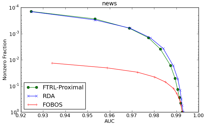
Figure 1: Sparsity versus accuracy tradeoffs on the 20 newsgroups dataset. Sparsity increases on the y-axis, and AUC increases on the x-axis, so the top right corner gets the best of both worlds. FOBOS is pareto-dominated by FTRL-Proximal and RDA.

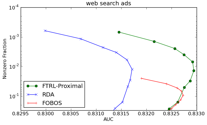
Figure 2: The same comparison as the previous figure, but on a large search ads ranking dataset. On this dataset, FTRL-Proximal significantly outperforms both other algorithms.

Fixing a particular value of $\lambda$, however, does not tell the whole story. For all these algorithms, one can trade off accuracy to get more sparsity by increasing the $\lambda$ parameter. The best choice of this parameter depends on the application as well as the dataset. For example, if storing the model on an embedded device with expensive memory, sparsity might be relatively more important. To show how these algorithms allow different tradeoffs, we plot sparsity versus AUC for the different algorithms over a range of $\lambda$ values. Figure 1 shows the tradeoffs for the 20 newsgroups dataset, and Figure 2 shows the tradeoffs for web search ads.

In all cases, FOBOS is pareto-dominated by RDA and FTRL-Proximal. These two algorithms are almost indistinguishable in the their tradeoff curves on the newsgroups dataset, but on the ads dataset FTRL-Proximal significantly outperforms RDA as well.

6 Conclusions and Open Questions

The goal of this work has been to extend the theoretical understanding of several families of algorithms that have shown significant applied success for large-scale learning problems. We have shown that the most commonly used versions of mirror descent, FTRL-Proximal and RDA are closely related, and provided evidence that the non-smooth regularization $\Psi$ is best handled globally, via RDA or FTRL-Proximal. Our analysis also extends these algorithms to implicit updates, which can offer significantly improved performance for some problems, including applications in active learning and importance-weighted learning.

Significant open questions remain. The observation that FOBOS is using a subgradient approximation for much of the cumulative $L_{1}$ penalty while RDA and FTRL-Proximal handle it exactly provides a compelling explanation for the improved sparsity produced by the latter two algorithms. Nevertheless, this is not a proof that these two algorithms always produce more sparsity. Quantitative bounds on sparsity have proved theoretically very challenging, and any additional results in this direction would be of great interest.

Similar challenges exist with quantifying the advantage offered by implicit updates. Our bounds demonstrate, essentially, a one-step advantage for implicit updates: on any given update, the implicit update will increase the regret bound by no more than the explicit linearized update, and the inequality will be strict whenever the implicit update is non-trivial. However, this is insufficient to say that for any given learning problem implicit updates will offer a better bound. After one update, the explicit and implicit algorithms will be at different feasible points $x_{t+1}$, which means that they will suffer different losses under $f_{t+1}$ and (more importantly) compute and store different gradients for that function.

This issue is not unique to implicit updates: anytime the real loss functions $f_{t}$ are non-linear, but the algorithm approximates them by computing $g_{t}=\triangledown f_{t}(x_{t})$, two different first-order algorithms may see a different sequence of $g_{t}$’s; since tight regret bounds depend on this sequence, the bounds will not be directly comparable. Generally we assume the gradients are bounded, $\|g_{t}\|\leq G$, which leads to bounds like $\mathcal{O}(G\sqrt{T})$, but since a large number of algorithms obtain this bound, it cannot be used to discriminate between them. Developing finer-grained techniques that can accurately compare the performance of different first-order online algorithms on non-linear functions could be of great practical interest to the learning community since the loss functions used are almost never linear.

References

• Abernethy et al. (2008) Jacob Abernethy, Peter L. Bartlett, Alexander Rakhlin, and Ambuj Tewari. Optimal strategies and minimax lower bounds for online convex games. In COLT, 2008.
• Bartlett et al. (2007) Peter L. Bartlett, Elad Hazan, and Alexander Rakhlin. Adaptive online gradient descent. In NIPS, 2007.
• Beygelzimer et al. (2010) Alina Beygelzimer, Daniel Hsu, John Langford, and Zhang Tong. Agnostic active learning without constraints. In NIPS, 2010.
• Boyd and Vandenberghe (2004) Stephen Boyd and Lieven Vandenberghe. Convex Optimization. Cambridge University Press, 2004.
• Chang and Lin (2010) Chih-Chung Chang and Chih-Jen Lin. LIBSVM data sets. http://www.csie.ntu.edu.tw/~cjlin/libsvmtools/datasets/, 2010.
• Do et al. (2009) Chuong B. Do, Quoc V. Le, and Chuan-Sheng Foo. Proximal regularization for online and batch learning. In ICML, 2009.
• Dredze (2010) Mark Dredze. Multi-domain sentiment dataset (v2.0). http://www.cs.jhu.edu/~mdredze/datasets/sentiment/, 2010.
• Duchi and Singer (2009) John Duchi and Yoram Singer. Efficient learning using forward-backward splitting. In NIPS. 2009.
• Duchi et al. (2010a) John Duchi, Elad Hazan, and Yoram Singer. Adaptive subgradient methods for online learning and stochastic optimization. In COLT, 2010a.
• Duchi et al. (2010b) John Duchi, Shai Shalev-Shwartz, Yoram Singer, and Ambuj Tewari. Composite objective mirror descent. In COLT, 2010b.
• Hazan (2008) Elad Hazan. Extracting certainty from uncertainty: Regret bounded by variation in costs. In COLT, 2008.
• Kakade et al. (2009) Sham M. Kakade, Shai Shalev-shwartz, and Ambuj Tewari. On the duality of strong convexity and strong smoothness: Learning applications and matrix regularization. 2009.
• Kalai and Vempala (2005) Adam Kalai and Santosh Vempala. Efficient algorithms for online decision problems. Journal of Computer and Systems Sciences, 71(3), 2005.
• Karampatziakis and Langford (2010) Nikos Karampatziakis and John Langford. Importance weight aware gradient updates. http://arxiv.org/abs/1011.1576, 2010.
• Kivinen and Warmuth (1997) Jyrki Kivinen and Manfred Warmuth. Exponentiated Gradient Versus Gradient Descent for Linear Predictors. Journal of Information and Computation, 132, 1997.
• Kivinen et al. (2006) Jyrki Kivinen, Manfred Warmuth, and Babak Hassibi. The p-norm generalization of the lms algorithm for adaptive filtering. IEEE Transactions on Signal Processing, 54(5), 2006.
• Kulis and Bartlett (2010) Brian Kulis and Peter Bartlett. Implicit online learning. In ICML, 2010.
• Lee et al. (2006) Su-In Lee, Honglak Lee, Pieter Abbeel, and Andrew Y. Ng. Efficient l1 regularized logistic regression. In AAAI, 2006.
• McMahan (2010) H. Brendan McMahan. Follow-the-Regularized-Leader and Mirror Descent:
Equivalence Theorems and L1 Regularization.
Submitted, 2010.
• McMahan and Streeter (2010) H. Brendan McMahan and Matthew Streeter. Adaptive bound optimization for online convex optimization. In COLT, 2010.
• Shalev-Shwartz and Kakade (2008) Shai Shalev-Shwartz and Sham M. Kakade. Mind the duality gap: Logarithmic regret algorithms for online optimization. In NIPS, pages 1457–1464, 2008.
• Shalev-Shwartz and Singer (2006) Shai Shalev-Shwartz and Yoram Singer. Convex repeated games and fenchel duality. In NIPS, 2006.
• Streeter and McMahan (2010) Matthew J. Streeter and H. Brendan McMahan. Less regret via online conditioning. http://arxiv.org/abs/1002.4862, 2010.
• Sugiyama et al. (2008) Masashi Sugiyama, Taiji Suzuki, Shinichi Nakajima, Hisashi Kashima, Paul Bünau, and Motoaki Kawanabe. Direct importance estimation for covariate shift adaptation. Annals of the Institute of Statistical Mathematics, 60(4), 2008.
• Xiao (2009) Lin Xiao. Dual averaging method for regularized stochastic learning and online optimization. In NIPS, 2009.
• Xiao (2010) Lin Xiao. Dual averaging methods for regularized stochastic learning and online optimization. Journal of Machine Learning Research, 11, 2010.
• Zinkevich (2003) Martin Zinkevich. Online convex programming and generalized infinitesimal gradient ascent. In ICML, 2003.
• Zinkevich (2004) Martin Zinkevich. Theoretical guarantees for algorithms in multi-agent settings. PhD thesis, Pittsburgh, PA, USA, 2004.