IPMU-10-0156

Dynamical Cobordisms
in
General Relativity and String Theory

Simeon Hellerman¹ and Matthew Kleban²

¹Institute for the Physics and Mathematics of the Universe
The University of Tokyo
Kashiwa, Chiba 277-8582, Japan
²Center for Cosmology and Particle Physics
New York University
4 Washington Place
New York, NY 10003

Abstract

We describe a class of time-dependent solutions in string- or M-theory that are exact with respect to ${\alpha^{\prime}}{}$ and curvature corrections and interpolate in physical space between regions in which the low energy physics is well-approximated by different string theories and string compactifications. The regions are connected by expanding “domain walls” but are not separated by causal horizons, and physical excitations can propagate between them. As specific examples we construct solutions that interpolate between oriented and unoriented string theories, and also between type II and heterotic theories. Our solutions can be weakly curved and under perturbative control everywhere and can asymptote to supersymmetric at late times.

1 Introduction

The great majority of research in string theory has focused on supersymmetric, time-independent configurations. Such solutions generally do not admit domain walls that interpolate between different string theories. However, when one relaxes these strictures even slightly, a much larger range of solutions becomes available. For example [5, 6, 7, 8, 9, 10] demonstrated that non-supersymmetric string theories are dynamically connected to supersymmetric vacua by tachyon condensation. In [1], one of us showed that the global F-theory constraint that there be no more than 24 7-branes is lifted if the space is expanding, even in the simplest case where the expansion is homogeneous and without acceleration.

In this note we will use an ansatz similar to [1, 2] to demonstrate that the mild form of SUSY breaking induced by a uniform, constant velocity expansion suffices to allow regions containing a very wide variety of effective string theories to simultaneously co-exist in the same causally connected physical space. The main examples we consider are locally flat space, and so (thought of as string solutions) are ${\alpha^{\prime}}{}$-exact. However the expanding space has non-trivial topology, and at early times when its cycles are small quantum effects will become important. We will not attempt to study our solutions at early times; instead, we will focus on their medium and late time behavior (but see [11, 12, 13, 14, 15, 16]).

Our solutions have implications for the string theory landscape [27], which in turn plays a crucial role in stringy cosmology. The application of landscape ideas to cosmology requires that the large number of vacua in string theory admit dynamical solutions interpolating among them. The best known such solutions are Coleman-de Luccia instantons [28] and their string-theoretic cousins, the Euclidean D-brane solutions that interpolate among flux vacua [29, 31]. Some of the most phenomenologically promising compactifications of string theory are the F theory solutions sketched in [32] and refined in subsequent work. Dynamical solutions have been found [33, 34] describing transitions from such vacua to other vacua with different flux numbers, or to noncompact ten-dimensional space altogether.

At present, very little is understood about cosmological interpolating solutions beyond the level of effective field theory. The description of such solutions in terms of low-energy dynamics of general relativity coupled to matter is useful for some calculations, but is limited to studying transitions in a regime where the transition generates only small perturbations on the background spacetime. As a result, effective field theory may not be capable of describing transitions in which the solution changes qualitatively, for example in terms of topology or other gross features. And yet, the use of the landscape as a theoretical tool requires the study of transitions among such qualitatively different vacua.

A related issue is that all realistic string vacua [32] involve orientifolds as an essential ingredient in their construction. In perturbation theory, string orientifolds have no dynamics associated with them. Consequently, the known solutions that interpolate between realistic vacua do not change the number, type or geometry of orientifolds. In order to connect realistic, KKLT-type vacua to the rest of the solution space of string theory, it must be possible to find interpolating solutions that do change the features of the orientifolds. We will exhibit an explicit example of such a solution.

Some controlled examples of interpolating solutions have been constructed in string theory that change not only the geometry of space, but the total number of spacetime dimensions and the kind of string theory altogether. These solutions are not instantons, but instead involve real-time cosmological solutions interpolating from an unstable solution to a stable vacuum or another unstable one ([3, 4, 5, 6, 7, 8, 9, 10]). Though not realistic as string cosmologies, these solutions demonstrate that interpolating cosmological solutions among string vacua exist, and can be controlled and solved exactly even when they describe changes to the background that are not small perturbations of a fixed geometry.

The solutions presented here differ from these in several ways, among them that the interpolation is spacelike—the different solutions coexist in regions separated by spacelike connecting regions. Specifically we make use of the theory of cobordisms, focusing on the case where the cobordism manifold is hyperbolic, to investigate how the topology of the compact dimensions can vary continuously from region to region in the universe. An interesting fact is that this mechanism involves only classical geometry, without direct inputs from string theory. After developing this framework, we will apply it to construct a solution interpolating between oriented and unoriented string theories. In all the cases we consider there are no horizons in our geometries; the different regions are causally connected and the domain walls separating them are traversible.

2 Riemann surfaces

Begin with the Milne-type metric

$$ds^{2}=-dt^{2}+t^{2}dH_{n}^{2}+ds_{m}^{2},$$ (2.1)

where $dH_{n}^{2}$ is the metric on the unit $n$-dimensional hyperbolic space (the maximally symmetric $n$-space with constant negative curvature), $ds_{m}^{2}$ is some Ricci-flat $m$-manifold, $t$ is time, and $D=n+m+1$ is the total spacetime dimension. As can be easily seen this metric is constitutes an exact solution to the vacuum Einstein equations with vanishing cosmological constant, assuming the internal metric $ds_{m}^{2}$ is such a solution as well. In fact, the first two terms in the metric constitute the Milne coordinatization of Minkowski space. Since the Friedmann-Robertson-Walker scale factor of the expanding part of the metric is $a(t)=t$, the corresponding Hubble length is just $t$, as is the proper radius of curvature of the hyperbolic spatial sections.

Hyperbolic $n$-space, being maximally symmetric, has a large isometry group: $SO(n,1)$, with $n(n+1)/2$ generators. One can construct topologically non-trivial, locally hyperbolic spaces by identifying $H_{n}$ under the action of a discrete subgroup $\Gamma$ of the isometry group. The result is a space that can have either finite or infinite volume, and, if the subgroup action is properly discontinuous (no fixed points), the space is smooth and free of singularities or defects.

Because the spatial slices remain locally hyperbolic after the identification, the resulting spacetime is still locally flat and therefore a vacuum solution to Einstein’s equations and an ${\alpha^{\prime}}{}$-exact solution in string theory. However the presence of non-trivial topology means that the full space is no longer globally Minkowski space, and the physics is time-dependent. At early times, the lengths of the smallest non-contractible cycles of the space become small. The curvature of the spatial slices becomes large both in string and in Planck units, and the physics is non-perturbative. We will focus on later times, where perturbative effects are small and the solution is under full control. As time passes the cycles grow larger and the solution becomes closer and closer to flat and more and more supersymmetric.

As we will discuss later, for $n>3$ one can consider more general spacetimes where the locally hyperbolic space is replaced by a general Einstein manifold with constant negative curvature. In that case the full spacetime is a solution at least to lowest order in ${\alpha^{\prime}}{}$.

2.1 Worldwide pants: The expanding triniverse

To illustrate the possibilities allowed by this class of solutions we begin with a very simple case: $n=2$, choosing the subgroup $\Gamma$ so that the space $X={\hbox{$\,\vrule height=6.45831pt,width=0.4pt,depth=0.0pt\kern-3.00003pt{\rm H}$}}_{2}/\Gamma$ is a pair of pants: a non-compact Riemann surface with Euler character $-1$, a hyperbolic metric, and a hyperbolic boundary that consists of three disconnected circles (Figure 1). In appendix A we explicitly construct the generators that realize this “hyperbolic trinion”; $\Gamma$ is a freely acting, finitely generated subgroup of $PSL(2,{\rm I\kern-1.79993ptR})$ in which every non-identity element is hyperbolic. For simplicity we focus on the case where the trinion has a $\mathchoice{\hbox{\cmss Z\kern-3.99994ptZ}}{\hbox{\cmss Z\kern-3.99994ptZ}}{\lower 0.9pt\hbox{\cmsss Z\kern-2.79996ptZ}}{\lower 1.2pt\hbox{\cmsss Z\kern-2.79996ptZ}}_{3}$ symmetry that rotates the legs, in which case it turns out to have only a single real modulus preserving the symmetry. For now we will treat the $m$-dimensional transverse space as 7-dimensional Euclidean space, having in mind weakly coupled critical string theory.

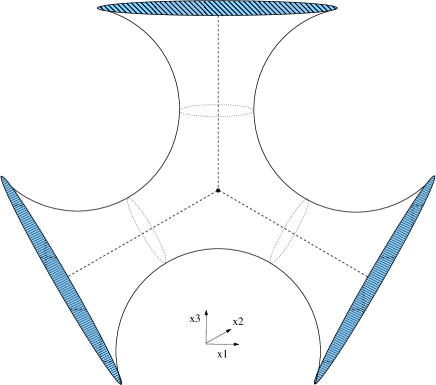
Figure 1: The trinion, or pair of hyperbolic pants. The dashed circles indicate the three garters—minimum length geodesics wrapping the legs.

The 2+1 dimensional part of the spacetime (2.1) is a homogeneous but anisotropic comology. The spatial slices are the surfaces $X$, which expand homogeneously at constant velocity (with scale factor $a(t)=t$). The metric on ${\hbox{$\,\vrule height=6.45831pt,width=0.4pt,depth=0.0pt\kern-3.00003pt{\rm H}$}}_{2}$ is the Poincaré metric

$$\begin{array}[]{c}ds^{2}={{dx^{2}+dy^{2}}\over{y^{2}}}={{dz\,d{\bar{z}}}\over{{\rm Im}(z)^{2}}}={{dr^{2}}\over{r^{2}\,{\rm sin}^{2}\theta}}+{{d\theta^{2}}\over{{\rm sin}^{2}\theta}}\ ,\end{array}$$ (2.3)

where

$$\begin{array}[]{c}z=x+iy=r\,{\rm exp}\left({i\theta}\right)\ ,\hskip 36.135pt{\bar{z}}=x-iy=r\,{\rm exp}\left({-i\theta}\right)\ .\end{array}$$ (2.5)

The Poincaré metric has Gaussian curvature $-1$, or Ricci scalar curvature $-2$. The slices have constant negative curvature and thus the vacuum Einstein equations are satisfied automatically for our choice of scale factor, for any choice of $\Gamma$.

Prior to taking the quotient by $\Gamma$, the 2+1 dimensional part of the spacetime is simply Minkowski space, which means that our cosmological solution is a quotient of Minkowski space by a discrete subgroup of the three-dimensional Poincaré group acting on ${\rm I\kern-1.79993ptR}^{2,1}$. This guarantees that the spacetime solves not only the equations of classical general relativity, but is also a tree-level solution to string theory to all orders in ${\alpha^{\prime}}{}$, assuming the transverse $7$-dimensional factor is also an ${\alpha^{\prime}}{}$-exact CFT. This is a somewhat similar situation to that of [19, 20, 21] in that the description of the spacetime as a quotient of Minkowski space by a subgroup of the isometry group guarantees its existence as a tree-level solution to string theory, with corrections coming only from higher-genus amplitudes. The loop corrections in our cosmology are more important than in [20, 21], since there the subgroup is parabolic and preserved a lightlike Killing vector, and therefore has vanishing particle production from the vacuum. The group $\Gamma$ that corresponds to a trinion is hyperbolic, has no timelike or lightlike Killing vector, and allows particle production from the vacuum due to higher-genus effects. However we will only consider our solution at tree-level in string theory; as with many FRW cosmologies in string theory and field theory, there is a Big Bang singularity at which quantum effects are potentially important, but any particle production from the initial singularity is irrelevant at late times, as any density of produced particles is rapidly redshifted away by the expansion of the universe.

As we will see, with an appropriate choice of moduli and spin structure, this space can describe a universe in which the physics in different regions is approximated by a static supersymmetric or non-supersymmetric string theory. These regions are connected by a Hubble-sized piece of spacetime that functions qualitatively like a “domain wall”, in the sense that it separates regions with differing effective physics. If in addition to modding by $\Gamma$ one performs an orientifold projection, the space describes a domain wall connecting a region of oriented string theory to an unoriented string theory.

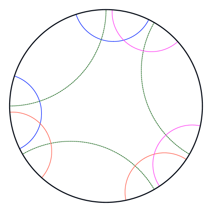
Figure 2: A $\mathchoice{\hbox{\cmss Z\kern-3.99994ptZ}}{\hbox{\cmss Z\kern-3.99994ptZ}}{\lower 0.9pt\hbox{\cmsss Z\kern-2.79996ptZ}}{\lower 1.2pt\hbox{\cmsss Z\kern-2.79996ptZ}}_{3}$ symmetric trinion as a quotient of the Poincare disk. Solid curves of the same hue are identified. The dashed lines are minimal length geodesics; cutting along them would produce a pair of hyperbolic pants with the skinniest possible cuffs and waist.

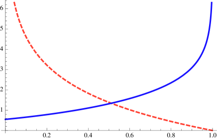
Figure 3: The solid curve is the geodesic distance from either $Z_{3}$ fixed point to the minimum length geodesic wrapping a leg (the garter) as a function of the modulus $\gamma$ (see Appendix A for details). The dashed curve is the geodesic circumference $L$ of the garter, and also the geodesic distance around the crotch (the zipper) between the two $Z_{3}$ fixed points. In the limit of interest the garter moves very far from the center, the leg gets very skinny ($L\rightarrow 0$), and the size of the center (measured by the distance between the two $Z_{3}$ symmetric points) also gets small.

2.2 Garter theory

Each leg of the hyperbolic trinion (Fig. 1) has a geodesic “garter” where the 1-cycle wrapping the leg attains its minimum co-moving length $L$. As we demonstrate in Appendix A, we can choose the modulus of the $\mathchoice{\hbox{\cmss Z\kern-3.99994ptZ}}{\hbox{\cmss Z\kern-3.99994ptZ}}{\lower 0.9pt\hbox{\cmsss Z\kern-2.79996ptZ}}{\lower 1.2pt\hbox{\cmsss Z\kern-2.79996ptZ}}_{3}$ symmetric trinion to set $L$ to any value from zero to infinity (Fig. 3). In particular we can choose $L<\hskip-5.78172pt<1$ (recall that our hyperbolic space has unit comoving curvature) so that the garter’s length is very small in units of the spatial curvature.

The proper length around the garter in the expanding metric (2.1) is $a(t)L=tL$, and the proper radius of curvature of the spatial slices is simply $t$. Hence if we choose the modulus so that $L<\hskip-5.78172pt<1$, the physical length of the geodesic will always remain small in units of the physical spatial curvature. However if there is some fixed physical length scale in the dynamics, such as the string length $\sqrt{{\alpha^{\prime}}{}}$, the proper radius of the garter will always exceed it at sufficiently late times. Nevertheless, as we will see small $L$ means that the physics in the vicinity of the garter can be well-described as a compactification on a small circle for very long times and over very long distance scales.

The space in a particular leg is locally a circle fibered over an interval, with metric

$$ds_{2}^{2}=-dt^{2}+t^{2}\left(~{}du^{2}+L^{2}\,{\rm cosh}^{2}u\,d\chi^{2}\right)\ ,$$ (2.6)

where $\chi$ is identified with $\chi+1$ (c.f. Eq. A.3). The constant $L$ is a parameter of the solution, expressing the comoving length of the garter in units of the spatial curvature. The limit of interest is $L<\hskip-3.61371pt<1$.

For small $u$ the space is an expanding cylinder. A feature of the small $L$ limit of the modulus is that the region near the minimum length geodesic is many Hubble lengths away from the center of the trinion (Fig. 3). In that limit the space remains approximately a small circle cross an interval over a very large distance.

It is illuminating to consider the metric at late times, $t\simeq t_{0}>>1$, expressing the comoving length $L$ in terms of the proper radius of the circle, as $L=2\pi{\tt r}_{0}/t_{0}$ and exchanging the comoving transverse coordinate $u$ for the proper transverse coordinate $v\equiv u\,t_{0}$. Then, restoring the factors of the speed of light $c$, the metric becomes

$$\begin{array}[]{c}ds_{2}^{2}=-c^{2}\,dt^{2}+(t^{2}/t_{0}^{2})\,\left(~{}dv^{2}+4\pi^{2}{\tt r}_{0}^{2}\,{\rm cosh}^{2}\left(~{}{{v}\over{c\,t_{0}}}\right)\,d\chi^{2}\,\right)\ .\end{array}$$

The garter lies at $v=0$. The approximate metric near the garter is

$$ds_{2}^{2}=-c^{2}\,dt^{2}+(t^{2}/t_{0}^{2})\,\left[~{}dv^{2}+4\pi^{2}{\tt r}_{0}^{2}\,\left(~{}1+{{v^{2}}\over{2\,c^{2}t_{0}^{2}}}\right)d\chi^{2}\right]+{\cal O}({{{\tt r}_{0}^{2}\,v^{4}}\over{t_{0}^{4}}})\,.$$ (2.8)

In the vicinity of the garter, string theory on this space has a spectrum of winding and and Kaluza-Klein modes, with mass-squared given by

$$\begin{array}[]{c}m^{2}=M_{10}^{2}+{{\hbar^{2}n_{KK}^{2}}\over{c^{2}{\tt r}^{2}}}+{{\hbar^{2}w^{2}{\tt r}^{2}}\over{c^{2}{\alpha^{\prime}}{}^{2}}}\ ,\end{array}$$

where ${\tt r}\equiv{{{\tt r}_{0}t}\over{t_{0}}}\,{\rm cosh}\left(~{}{{v}\over{c\,\tau_{0}}}\right)$ is the local radius of the $\chi$ circle, $M_{10}^{2}$ is the ten-dimensional mass-squared of the string mode, and $n_{KK}$ and $w$ are the Kaluza-Klein number and winding number of the mode around the $\chi$-circle.

The winding modes feel a confining potential due to the fact that the radius of the compact circle grows quadratically with the coordinate $u$ as one moves away from the garter; conversely, KK modes feel a repulsive quadratic potential. However the gradient of this potential is weak and $L$-independent, so that the time scale of the instability for KK modes is only Hubble.

To see this, examine the proper acceleration

$$\begin{array}[]{c}{\rm acceleration}\simeq{{c^{2}}\over m}{{dm}\over{dv}}\end{array}$$

for a KK mode of a massless 10-dimensional field; the mass is $m_{{KK}}={{\hbar\,n_{KK}}\over{c\,{\tt r}}}$, so the acceleration at position $v$ will be

$${\rm acceleration}\simeq v/t_{0}^{2}\ ,$$ (2.11)

to lowest order in $v$, with corrections of order ${{v^{3}}\over{c^{2}\,t_{0}^{4}}}$. For $v$ in the vicinity of the garter $v<\hskip-3.61371pt<c\,H^{-1}$, a KK mode is approximately inertial over time scales comparable to the age of the universe.

The acceleration of a wound string has the same magnitude but the opposite sign. The magnitude of the proper acceleration of either a KK or wound string mode within a Hubble length of the garter is at most the Hubble acceleration. In the limit of interest to us ($H<\hskip-3.61371pt<m_{s}$), these accelerations are very slow.

The regions near distinct garters never go out of causal contact with each other; that is, there are no horizons in this cosmology. The scale factor $a(t)=t$ is the marginal case of FRW expansion with neither acceleration nor deceleration. The FRW time it takes light to propagate between two comoving points (such as two of the garters) is proportional to the start time and exponential in the comoving distance between the points (see Appendix A.2 for details).

A string mode created near one of the garters could be fired towards the crotch, resulting in (potentially painful) scattering and transmission amplitudes off the “domain wall” separating the legs. Amusingly, the worldsheet corresponding to this process would itself be a trinion that clothes the spacetime trinion. It would be interesting to study such processes, particularly in cases where the effective theories near the garters are very different (see below), but we will not pursue this further here.

2.3 Spin structure and dynamical stability

Let us now comment on the issue of the dynamical stability of our solution. Because of the expansion of the universe the question of “stability” must be treated with some care; the background is explicitly time-dependent. However if we focus on the dynamics in a garter region with ${\tt r}_{0}<\hskip-3.61371pt<c\,H^{-1}$, we can ask about dynamical stability on time scales of order ${\tt r}_{0}/c$, in which case the background can be treated as if it were static. As we have seen, in this limit each garter region becomes the product of a line (parametrized by $v$) and a circle (parametrized by $\chi$). So we can understand the dynamical stability of each region in terms of the limiting static compactification on $S^{1}$.

In this limit, the dynamical stability of the compactification is determined by the radius ${\tt r}_{0}$ of the circle, the amount of SUSY in the underlying theory, and the boundary conditions for the gravitini along the circle in a given garter region. If the underlying theory has a bulk tachyon—such as in type 0 or bosonic string theory—every garter region will be nonsupersymmetric.

If the underlying theory has ${\cal N}=1$ or ${\cal N}=2$ supersymmetry, then a garter region may be stable or unstable, depending on the size of the $\chi$-circle and the boundary conditions on the gravitini. If one or both gravitini are periodic around the $\chi$-circle, the garter region will have approximate ${\cal N}=1$ or ${\cal N}=2$ supersymmetry, respectively. The SUSY in this case is broken only by the overall expansion of the universe, so the scale of SUSY breaking $\hbar\,H$ is the same scale as that of the time-variation of the background itself.

If the underlying theory has ${\cal N}=1$ or ${\cal N}=2$ supersymmetry but both gravitini are antiperiodic around a given garter, the theory may still be tachyon-free, depending whether or not the radius ${\tt r}_{0}$ of the garter is large compared to the fundamental scale of the underlying gravity theory.

In the case of 11-dimensional ${\cal M}$-theory, a garter region with antiperiodic gravitini should be tachyon-free so long as the garter radius ${\tt r}_{0}$ is large compared to the only scale in the system, the $11$-dimensional Planck scale $L_{11}$. If ${\tt r}_{0}$ is much less then $L_{11}$ we expect that the effective 10-dimensional theory is described by type 0A string theory at weak coupling; according to the standard worldsheet analysis of this system, there is a tachyon with a rapid decay constant, $\Gamma_{\rm tachyon}=c\,\sqrt{{2\over{{\alpha^{\prime}}{}}}}$ (which in terms of 11-dimensional data[30] is proportional to $c\,L_{11}^{-{3\over 2}}\,{\tt r}_{0}^{+{1\over 2}}$).

In the case of 10-dimensional type IIA/B string theory with antiperiodic boundary conditions for all the fermions around the garter, the dynamical stability of the region can be analyzed systematically when the coupling is weak with string perturbation theory. Using the results of [22, 23] we see that the lowest winding string mode has mass $m^{2}=-{2\over{{\alpha^{\prime}}{}}}+{{{\tt r}_{0}^{2}}\over{{\alpha^{\prime}}{}^{2}}}$ at string tree level. So, for ${\tt r}_{0}>\sqrt{2{\alpha^{\prime}}{}}$, the compactification is tachyon-free at time $t_{0}$; for ${\tt r}_{0}<\sqrt{2{\alpha^{\prime}}{}}$ there is a vacuum instability with a decay rate of order $c/\sqrt{{\alpha^{\prime}}{}}$.

Even the tachyon-free regimes of 11-dimensional M-theory and 10-dimensional string theory with antiperiodic gravitini are not truly stable. There are nonperturbative gravitational instanton solutions [24] that allow a nonsupersymmetric leg to pinch off, disconnecting the asymptotic region from the 3-leg junction (although the action for such an instanton increases with the size ${\tt r}_{0}$ of the circle, so the integrated decay probability over all time will be finite). Furthermore, at one loop one expects that the mismatch of boundary conditions for bosons and fermions will lead to nonvanishing Casimir energies, generating a potential for the modulus ${\tt r}_{0}$ that scales as a power of ${\tt r}_{0}$ when ${\tt r}_{0}$ is large compared to the fundamental scale. In order to arrange truly stable dynamics, it is necessary for at least one gravitino to be periodic in each garter region.

How much freedom does one have to achieve such a configuration? For each spinor’s worth of local supersymmetry, one has the freedom to choose a spin structure determining the boundary conditions for fermions around the garter. Since in this example there are three garters (one on each leg of the trinion), naively there are three independent choices to make to determine the spin structure. In fact this is not quite correct: only two of the three cycles are homologically independent, so the the boundary conditions for fermions on the three cycles must satisfy a single relation—that the product of periodicities around all three garters multiply to -1 for each gravitino. The consequence is that either one or all three of the boundary conditions for a given gravitino field must be anti-periodic, as can easily be seen by considering the thrice-punctured sphere (the cycle that encircles all three punctures is contractible, and therefore fermions going around it must be anti-periodic). So it would seem that at least one of the three legs must always have “large” amount of supersymmetry breaking, characterized by the SUSY breaking scale $m_{KK}={1\over{{\tt r}_{0}}}$.

Such is the situation when one considers a theory with ${\cal N}=1$ supersymmetry (such as heterotic or type $I$ string theory in 10 dimensions or 11-dimensional $M$-theory). These theories do not admit solutions with supersymmetric boundary conditions in each leg of a three-universe junction. (We shall see later that this constraint is an artifact of a geometry with three asymptotic regions rather than another number, and can be evaded easily by adding extra legs to the Riemann surface.)

When one considers theories with ${\cal N}=2$ supersymmetry such as type IIA or IIB string theory, there are two independent 10D gravitini and two independent spinor fields’ worth of local SUSY, and therefore twice as many choices of spin structure on the trinion, one for each gravitino. Each spin structure must separately satisfy the consistency condition, with antiperiodic boundary conditions around at least one leg; however we have the freedom to choose the two gravitini to be antiperiodic around different legs, so that each leg has at least one periodic gravitino and therefore at least one dynamical supersymmetry preserved up to Hubble-scale effects.

For instance, we may choose the first set of gravitini to be periodic around garters A and B and antiperiodic around garter C, and the second set of gravitini to be periodic around garters B and C, and antiperiodic around garter A. The effective dynamics near garter $B$ has approximate ${\cal N}=2$ supersymmetry in $9$ dimensions, while the effective dynamics near garters $A$ and $C$ respect only ${\cal N}=1$ supersymmetry in $9$ dimensions. The latter is described by a chiral Scherk-Schwarz compactification of the type described in [17, 18]. Of course, the surviving SUSY in any region is merely approximate, being broken cosmologically by the overall expansion of the universe. But in the regime $L<\hskip-3.61371pt<1$ the distinction between a supersymmetric and nonsupersymmetric leg of the trinion is very sharp. In a supersymmetric leg, the SUSY breaking is Hubble-scale, with mass splittings at most of order $\Delta m\simeq H$ in each multiplet, whereas in the nonsupersymmetric legs the splittings would be of order $\Delta m\simeq{1\over{{\tt r}_{0}}}$.

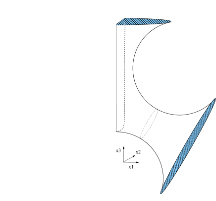
Figure 4: The orientitrinifold: the quotient of a three-legged Riemann surface by a $\mathchoice{\hbox{\cmss Z\kern-3.99994ptZ}}{\hbox{\cmss Z\kern-3.99994ptZ}}{\lower 0.9pt\hbox{\cmsss Z\kern-2.79996ptZ}}{\lower 1.2pt\hbox{\cmsss Z\kern-2.79996ptZ}}_{2}$ symmetry reflecting one pair of legs into one another, and the third leg into itself.

2.4 Orientifolds

If the trinion has a $\mathchoice{\hbox{\cmss Z\kern-3.99994ptZ}}{\hbox{\cmss Z\kern-3.99994ptZ}}{\lower 0.9pt\hbox{\cmsss Z\kern-2.79996ptZ}}{\lower 1.2pt\hbox{\cmsss Z\kern-2.79996ptZ}}_{2}$ symmetry that reflects one leg onto another, one can perform an orbifold or orientifold projection that maps the trinion into a space that connects a two asymptotic regions with different orientability properties for string worldsheets. For definiteness, arrange the trinion so that its legs lie in the $x_{2}-x_{3}$ plane, with one leg pointing along the positive $x_{3}$ axis, and the other two arranged to point at equal acute angles to the negative $x_{2}$ axis, as in Figure 1. There is a discrete symmetry ${\bf R}_{2}$ that leaves $x_{1}$ and $x_{3}$ unchanged, and reflects the $x_{2}$ coordinate. For the trinion embedded in Euclidean three space as in Figure 1, the reflection ${\bf R}_{2}$ acts as an antiholomorphic involution on the trinion, with a fixed locus of real dimension 1. The reflection ${\bf R}_{2}$ reflects legs A and C into one another, and reflects half of leg B into the other half. The fixed locus consists of a hairpin-shaped curve travelling down one side of leg B and up the other side – in pair-of-pants terminology, thinking of leg B as the waist of the pair of pants, the fixed locus coincides with the zipper, but extended infinitely as a geodesic along the front and back of the waist.

Now let us orientifold the pair of pants by the action of ${\bf R}_{2}$. Since the fixed locus has real codimension 1, this restricts us to type IIA string theory (unless we combine the action of ${\bf R}_{2}$ with some other action on the seven coordinates not involved in the cosmological solution). Since we are considering an orientifold, rather than an orbifold action, there are no consistency conditions on the action of ${\bf R}_{2}$ at string tree level other than the condition that the real codimension of the fixed locus be odd. At higher order in the string coupling, the tension and Ramond-Ramond charge of the O8-plane generate tadpoles for the dilaton, metric and Ramond-Ramond 10-form flux. To cancel the tadpole we can place 16 D8-branes along the locus of the O8-plane.

The orientifolded spacetime, then, is given by one half of the original spacetime—a fundamental region of the action of ${\bf R}_{2}$, with O8-plane boundaries and with coincident D8-branes as desired. Leg B (pointing along the positive $x_{3}$-axis) is reflected into itself by the action of ${\bf R}_{2}$, and so it is sliced in half by the orientifolding, with two O8-plane boundaries where leg B intersects the plane $x_{2}=0$. Legs A and C are symmetrically arranged on either side of $x_{2}=0$ and do not intersect it, so the reflection ${\bf R}_{2}$ reflects legs A and C into one another. Therefore, the geometry of the spacetime after orientifolding has two asymptotic regions: One asymptotic region points at an acute angle to the negative $x_{3}$ axis with the geometry of a circle fibered over a ray, and the other asymptotic region lies along the positive $x_{3}$ axis, with the geometry of an interval, with O8-plane boundaries, fibered along a ray. This geometry is depicted in Figure 4.

2.5 More general surfaces

Riemann surfaces with more than three legs

So far we have focused on the specific example of the hyperbolic trinion. Our construction extends equally well to Riemann surfaces obtained as quotients of ${\hbox{$\,\vrule height=6.45831pt,width=0.4pt,depth=0.0pt\kern-3.00003pt{\rm H}$}}_{2}$ by more complicated subgroups of $SL(2,{\rm I\kern-1.79993ptR})$. The closest generalization would be to free subgroups $\Gamma$ of $SL(2,{\rm I\kern-1.79993ptR})$ generated by $b-1$ elements, with every non-identity element of $\Gamma$ being hyperbolic and chosen such that the quotient $X\equiv{\hbox{$\,\vrule height=6.45831pt,width=0.4pt,depth=0.0pt\kern-3.00003pt{\rm H}$}}_{2}/\Gamma$ is a sphere with $b$ or more holes ($b\geq 4$). There are $3b-6$ real moduli describing the embedding of $\Gamma$ in $SL(2,{\rm I\kern-1.79993ptR})$: for each of the $b-1$ independent generators, there is a choice of element of $SL(2,{\rm I\kern-1.79993ptR})$, with each specified by three parameters. The freedom to conjugate the elements of the generating set by a general $SL(2,{\rm I\kern-1.79993ptR})$ matrix subtracts three parameters, leaving $3b-6$ real parameters specifying the identifications modulo coordinate transformations. We can equally well describe the geometry as the unique negatively curved metric on a Riemann surface described as a sphere with $b$ circular boundaries. The structure of the complex manifold in this description is specified by the locations of $b$ points, and the radii of the $b$ holes on the sphere, modulo an overall $SL(2,{\hbox{$\,\vrule height=6.45831pt,width=0.4pt,depth=0.0pt\kern-3.00003pt{\rm C}$}})$ transformation, for a total of $2b+b-6=3b-6$ real parameters. We can of course impose additional discrete symmetries to cut down the number of moduli, and we can orbifold or orientifold by these symmetries if we choose.

Any such Riemann surface $X$ generates an exact solution of the vacuum Einstein equations and an ${\alpha^{\prime}}{}$-exact solution of string theory, as was the case for the trinionic spatial slices we discussed earlier. The metric

$$\begin{array}[]{c}ds^{2}_{\rm FRW}=-dt^{2}+t^{2}\,ds_{X}^{2}\end{array}$$

is an orbifold of $2+1$-dimensional Minkowski space by a discrete group $\Gamma$, and thus gives rise to a direct construction of an exactly conformal 2-dimensional worldsheet field theory describing string propagation.

The extension to $b$-universe junctions with $b>3$ makes it clear that the selection rules on boundary conditions for gravitini are very weak, and can in effect be evaded by adding additional asymptotic regions. The selection rule on spinor periodicities is that, if $\sigma_{a}$ is the periodicity of a gravitino around the garter in the $a^{\underline{\rm{th}}}$ leg (with $-1$ for antiperiodic fermions and $+1$ for periodic fermions), then the set of periodicities must satisfy

$$\begin{array}[]{c}\prod_{a=1}^{b}\,(-\sigma_{a})=+1\ .\end{array}$$

In particular, for $b$ even it is possible to choose all garter regions to be supersymmetric.

Solutions interpolating between type IIA and $E_{8}\times E_{8}$ heterotic string theory

Combined with the freedom to take $\mathchoice{\hbox{\cmss Z\kern-3.99994ptZ}}{\hbox{\cmss Z\kern-3.99994ptZ}}{\lower 0.9pt\hbox{\cmsss Z\kern-2.79996ptZ}}{\lower 1.2pt\hbox{\cmsss Z\kern-2.79996ptZ}}_{2}$ quotients with codimension-1 fixed planes, the case $b=4$ of the geometry discussed above gives us a construction of interpolating solutions between supersymmetric regions of different types in theories with ${\cal N}=1$ supersymmetry, in particular 11-dimensional M-theory.

We begin with a Riemann surface with four legs (depicted in Figure 5), and a set of reflection symmetries realized in a particular way. To describe the symmetries conveniently we embed the surface in three-dimensional Euclidean space, with axes labelled $x_{1,2,3}$. The two legs pointing in the negative $x_{1}$-direction are arranged to lie in the $x_{1}-x_{3}$ plane, while the two legs pointing in the positive $x_{1}$ direction are arranged to lie in the $x_{1}-x_{2}$ plane. One reflection symmetry (${\bf R}_{2}$) fixes $x_{1}$ and $x_{3}$, and reflects the $x_{2}$ coordinate, while the other reflection symmetry (${\bf R}_{3}$) fixes $x_{1}$ and $x_{2}$, and reflects the $x_{3}$ coordinate. Both symmetries act as antiholomorphic involutions on the Riemann surface, with fixed loci of real codimension 1. The reflection ${\bf R}_{3}$ reflects the first pair of legs into one another, and reflects each of the second pair of legs into itself, while the reflection ${\bf R}_{2}$ reflects the second pair of legs into one another, and reflects each of the first pair of legs into itself.

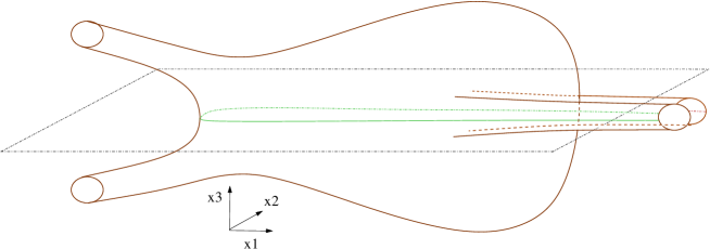
Figure 5: A Riemann surface with four hyperbolic legs, has the geometry of a whale with two $\mathchoice{\hbox{\cmss Z\kern-3.99994ptZ}}{\hbox{\cmss Z\kern-3.99994ptZ}}{\lower 0.9pt\hbox{\cmsss Z\kern-2.79996ptZ}}{\lower 1.2pt\hbox{\cmsss Z\kern-2.79996ptZ}}_{2}$ symmetries. Each $\mathchoice{\hbox{\cmss Z\kern-3.99994ptZ}}{\hbox{\cmss Z\kern-3.99994ptZ}}{\lower 0.9pt\hbox{\cmsss Z\kern-2.79996ptZ}}{\lower 1.2pt\hbox{\cmsss Z\kern-2.79996ptZ}}_{2}$ symmetry factor exchanges one pair of legs and reflects each of the other pair into itself. A quotient by one of the $\mathchoice{\hbox{\cmss Z\kern-3.99994ptZ}}{\hbox{\cmss Z\kern-3.99994ptZ}}{\lower 0.9pt\hbox{\cmsss Z\kern-2.79996ptZ}}{\lower 1.2pt\hbox{\cmsss Z\kern-2.79996ptZ}}_{2}$ symmetries has a single leg with circular cross-section and two legs with interval cross sections.

Having defined this Riemann surface and the associated cosmological solution of general relativity/string/M-theory, we can orbifold the solution by one of its two reflection symmetries, say ${\bf R}_{3}$. The resulting quotient has a single cylindrical leg with closed circular cross-sections in the asymptotic region at negative $x_{1}$, and two regions which are topologically intervals fibered over a ray in the asymptotic region at positive $x_{1}$. This geometry is a consistent exact solution of any gravity theory that allows orbifolding by a reflection with a real codimension-1 fixed locus, adding branes for tadpole cancellation as necessary. Theories allowing such orbifolding/orientifolding include type IIA string theory and 11-dimensional M-theory.

The case of M-theory on such an orbifold is particularly interesting, as it is known [25, 26] that codimension-1 orbifold fixed planes in M-theory support propagating $E_{8}$ gauge symmetries. M-theory compactified on an interval bounded by such fixed loci is described by weakly coupled $E_{8}\times E_{8}$ heterotic string theory in the limit where the length $\pi{\tt r}_{0}$ of the interval at its minimum is much smaller than the 11-dimensional Planck length $L_{11}$, assuming the boundary conditions on the gravitini are supersymmetric, as we have arranged them to be in this case.

This geometry, and its realization as the spatial section of an FRW metric, gives an explicit construction of a controlled solution of M theory that realizes dramatically different phases of the theory in different regions of the universe; one asymptotic region is described by the dynamics of type IIA string theory, where the other two asymptotic regions are described by the dynamics of heterotic string theory. The size of the interval and that of the circle grow exponentially away from the garter region. However the exponential growth as a function of distance from the garter is slow, with variation only on Hubble distances. Thus if we tune all the garter lengths to be much smaller than the 11D Planck scale, then at late times we have macroscopically sized regions of different superstring theories realized in different regions of the same universe, all causally connected to one another. There is no contradiction from the point of view of string theory, as there is always a region in the middle that is strongly coupled from the point of view of either set of string degrees of freedom. Nonetheless the solution at late times is protected from quantum corrections due to the hierarchy between the Hubble scale and the Planck scale in the regions where the geometry is large, and the residual supersymmetry in the regions where the geometry is small.

Cusps and parabolic quotients

So far we have studied the physics near the garter of one of the legs of a multi-legged, negatively curved Riemann surface. It is also illuminating to expand around one of the legs away from the minimum at the garter. Expanding $u$ around $u_{0}>0$ as $u=u_{0}+\epsilon$ with $u_{0}>\hskip-3.61371pt>1$, $\cosh(u)\approx e^{u_{0}+\epsilon}/2$ and the metric (2.6) becomes

$$\begin{array}[]{c}ds_{2}^{2}\approx-dt^{2}+t^{2}\left[d\epsilon^{2}+\left({Le^{u_{0}}/2}\right)^{2}\left(1+2\epsilon+{\cal O}(\epsilon^{2})\right)\right]d\chi^{2}.\end{array}$$

The space near the garter $u=0$ is symmetric under reflections in $u$, which results in a quadratic potential for winding and KK modes. Instead here there is a linear term in the potential and no symmetric point—evaluating the proper acceleration of a KK or winding mode, one finds simply

$$\begin{array}[]{c}{d\ln(m_{KK})/(td\epsilon)}\approx 1/t=H.\end{array}$$

So even away from the garter the variation in the leg radius can be neglected, at least for times and distances short compared to the Hubble scale. When $Le^{u_{0}}$ is sufficiently small, at time $t_{0}$ the physics within a Hubble radius of $u=u_{0}$ will be well approximated by the KK reduction of a circle of physical size $t_{0}Le^{u_{0}}$.

As we will discuss briefly below, hyperbolic manifolds generically develop regions known as cusps in singular limits of their moduli spaces. These “thin” regions have metric

$$\begin{array}[]{c}ds_{n}^{2}\approx du^{2}+e^{2u}ds_{n-1}^{2}.\end{array}$$

If the cusp cross-section $ds_{n-1}^{2}$ is flat (for example a torus), this is locally hyperbolic space.

Expanding as before around some point $u=u_{0}$, we have just seen that if $t_{0}L_{i}e^{u_{0}}$ is sufficiently small (where $L_{i}$ is the comoving length of some cycle in $ds_{n-1}^{2}$) we can reduce on that cycle. This provides a very general method for constructing ${\alpha^{\prime}}{}$ exact interpolating string solutions in higher dimensions.

3 Higher dimensions

Our ansatz (2.1) was

$$ds^{2}=-dt^{2}+t^{2}ds_{n}^{2}+ds_{m}^{2},$$ (3.17)

where so far we have considered cases in which $ds_{n}^{2}$ is a Riemann surface. More generally if $ds_{n}^{2}$ is a locally hyperbolic (constant negative sectional curvature) manifold, and $ds_{m}^{2}$ is $m$-dimensional Euclidean space, an orbifold of it, a Calabi-Yau, a product of those, or some other exactly conformal sigma model, this metric is an $\alpha^{\prime}$-exact solution to string theory (and a solution to supergravity with no higher curvature corrections to the $n+1$-dimensional factor of the geometry.)

Instead of ${\alpha^{\prime}}{}$-exactness we could require merely that the metric solve the low energy equations of string or M-theory, i.e. Einstein’s equations plus the equations of motion for the other massless fields. In that case the $n$-dimensional space $ds_{n}^{2}$ need not be hyperbolic. Instead, it should satisfy

$$R_{n}^{ij}=-(n-1)g_{n}^{ij},$$ (3.18)

where $i,j\in 1,..,n$ run over the indices of $ds_{n}^{2}$; i.e. it should be an Einstein manifold with Ricci scalar $R=-n(n-1)<0$. If in addition $ds_{m}^{2}$ is Ricci flat, one can easily verify that the full spacetime satisfies $R_{\mu\nu}=0$, where $\mu$ and $\nu$ run over all coordinates. In dimensions $n=2$ and 3 Einstein with negative curvature is equivalent to locally hyperbolic (due to the absence of gravity waves), but for $n>3$ it is a weaker condition.

3.1 Cobordisms and their significance

By definition, the topology of a smooth manifold is exactly the collection of properties of the manifold that cannot be altered by deforming it in any smooth way. Therefore it may seem counter-intuitive that it should be possible to “interpolate smoothly” between two smooth manifolds of different topology, at least when classical notions of geometry and topology are in force. And yet it is indeed possible to do so.

By a smooth interpolation between two $n$-manifolds $X_{1,2}$ we mean a smooth $(n+1)$-manifold $Y$ such that the boundary of $Y$ is equal to the disconnected sum of $X_{1}$ and $X_{2}$, with the two components understood as having opposite orientation. There are many intuitive and easy-to-visualize examples in the case $n=1$. For instance, if $X_{1}$ is a circle and $X_{2}$ is the empty set $\emptyset$, then a cobordism $Y$ between $X_{1}$ and $X_{2}$ would be a smooth manifold $Y$ whose boundary is just the circle $X_{1}$ (such interpolating manifolds are quite familiar to physicists working on perturbative string theory).

Suppose we wish to find a solution in our class that interpolates between two string compactifications. In order for such a solution to exist, the two compactification manifolds must be cobordant. Moreover, the bordism manifold must admit a hyperbolic or negatively curved Einstein metric. In the following section we will briefly discuss under what conditions this is possible.

3.2 $n=2$

By the uniformization theorem, all Riemann surfaces with Euler character $\chi<0$ admit a hyperbolic metric. All 1-manifolds are cobordant to each other (although if spin structure is included, there is a $Z_{2}$ selection ruling requiring that the number of boundary components with period fermions must equal mod 2).

The trinion solution discussed above is an explicit example of such a hyperbolic cobordism, in that case between $S^{1}$ and $S^{1}\oplus S^{1}$. The orientifolded trinion interpolates between and interval and an $S^{1}$.

3.3 $n=3$

While all negatively curved Einstein 3-manifolds are hyperbolic, not all 3-manifolds admit such a metric, and those that do have a restricted structure. In fact the space of all 3-manifolds has been fully characterized through geometrization. All compact 3-manifolds can be decomposed into pieces of eight types: hyperbolic, spherical, Euclidean, and five other possibilities. In the case of interest for us—hyperbolic—much is known about the possible topologies and metric structures. For further details, see e.g. [38].

Because we are interested in regions of the hyperbolic 3-manifold where some cycles shrink, we can make use of the so-called “thick-thin” decomposition. This is a technique for dividing the manifold into a region where some cycle(s) get smaller than some universal $n$-dependent length (the “thin” part), and the rest of the manifold where all cycle(s) are large (the “thick” part).

The utility of this decomposition arises from the Margulis lemma, which restricted to $H_{2}$ and $H_{3}$ can be stated as follows:

There exists a number $\epsilon_{n}>0$ such that if $\Gamma$ is a discrete group of isometries of $H_{n}$ generated by $\gamma_{1},\gamma_{2},...,\gamma_{k}$ and there exists $p\in H_{n}$ such that $d(p,\gamma_{i}p)\leq\epsilon_{n}$, then $\Gamma$ is Abelian.

Here $n=2,3$, and $d(p_{1},p_{2})$ is the geodesic distance between the points $p_{1}$ and $p_{2}$, and the $\epsilon_{n}$ are ${\cal O}(1)$ constants depending only on the dimension $n$.

In the case of real surfaces $n=2$, Abelian $\Gamma$ means $\Gamma$ is generated by a single generator (since commuting elements of a Fuchsian group must share fixed points). For a smooth space the generator is either hyperbolic or parabolic. Therefore the “thin” part of any hyperbolic surface can be one of only two possibilities: either a garter (a circle cross an interval with “$\cosh$” warp factor) or a cusp (a circle cross an interval with decreasing exponential warp factor), where for the former the generator is hyperbolic, and for the latter, parabolic. The trinion has three thin regions of the first type (the three garters discussed above) connected by and to thick regions (the central junction and the hyperbolic trumpets that go off to the boundary—Figure 1).

The case of $n=3$ is somewhat more complex. The closest analog of the $n=2$ garter is a region of the space around a short closed geodesic cycle that is the axis of some hyperbolic generator in $\Gamma$. The space can be parametrized locally by distance along the geodesic cycle $\chi\simeq\chi+1$, an angle around the cycle $\theta\simeq\theta+2\pi$, and a radial distance $u$:

$$ds_{3}^{2}\sim du^{2}+\sinh^{2}(u)~{}d\theta^{2}+\cosh^{2}(u)~{}L^{2}d\chi^{2},$$ (3.19)

where $L<\epsilon_{3}$ is the distance around the cycle at its shortest point $u=0$ (the garter). As the radial distance $u$ increases, the length of the closed cycle grows as $\cosh u$. This type of thin region is compact; its boundary is a flat 2-torus.

The other type of thin part involves quotients by one or two parabolic elements. The metric on the thin part is

$$dz^{2}+e^{-2z}(dx^{2}+dy^{2})$$ (3.20)

where either one or both of $x$ and $y$ are identified under translations: $x\simeq x+L_{x}$, $y\simeq y+L_{y}$. These are cusps, where the cross-section of the cusp is either a cylinder ($L_{x}$ finite, $L_{y}$ infinite) or a torus (both $L_{x},L_{y}$ finite). In the latter case the thin part is non-compact but of finite volume.

The thin regions of hyperbolic type have topology $D^{2}\times S^{1}$, where the radius of the $S^{1}$ is minimum at the center of the disk—the garter—and increases (gradually, given an appropriate choice of moduli) as one moves radially out. The region within a Hubble length of the garter is two dimensional flat space cross a short closed cycle, and so one can reduce on the cycle and obtain a theory in two flat dimensions (parametrized by $u$ and $\theta$ in (3.19)), plus the transverse $m$ dimensions of (2.1).

On the other hand parabolic thin regions are 2-torii cross a semi-infinite interval, where the cycles of the torus can be made arbitrarily small by moving out along the cusp and have approximately constant size within a Hubble patch. Reducing on both cycles of the torus would give a theory in one dimension (parametrized by $z$ in (3.20)) plus the transverse $m$ dimensions. Hence a 3D hyperbolic manifold possessing thin regions of each type would connect effective theories in different numbers of dimensions and with different topology for the compact dimensions.

3.4 $n>3$

For $n>3$ we can restrict to locally hyperbolic manifolds if we would like to find $\alpha^{\prime}$-exact string solutions, or allow for general Einstein manifolds with negative curvature if we only require that the solutions be valid to lowest order in $\alpha^{\prime}$.

Locally hyperbolic n-manifolds:

The thick-thin classification above is effective for $n>3$, but there are more possibilities for the thin parts. Roughly speaking they are either the obvious generalization of the garter case discussed above for $n=3$ (the space near the garter is Euclidean $n-1$ space $E_{n-1}$ cross a small circle, with the size of the circle growing like cosh as one moves away from the origin of the Euclidean space), or cusps with cross-sections that are orbifolds of $E_{n-1}$. Those include $(n-1)$-torii, and hyperelliptic surfaces and their higher and odd-dimensional relatives.

Negatively curved Einstein manifolds:

In the case $n=4$ there are some mild conditions on the topology of Einstein manifolds with negative curvature [40]. However for $n>4$ there are no known restrictions: it may be that all compact $n$-manifolds with $n>4$ admit negatively curved Einstein metrics. If so, we can connect nearly any collection of $n-1$-manifolds using our expanding solution. Of course (since this is a topological statement) one is not guaranteed that the geometry of the $n-1$ manifolds can be adjusted as desired. But given the considerable freedom available, it seems likely that any or nearly any string compactification on (for example) an $n-1=6$ manifold can be approximately realized locally and connected to any other such compactification by a negatively curved Einstein 7-manifold. In fact it seems plausible that the entire vacuum landscape of string and M-theory can be connected this way.

4 Conclusions

There are a number of directions it would be interesting to pursue. Among them would be to study string scattering between different regions of the expanding triniverse or its $\mathchoice{\hbox{\cmss Z\kern-3.99994ptZ}}{\hbox{\cmss Z\kern-3.99994ptZ}}{\lower 0.9pt\hbox{\cmsss Z\kern-2.79996ptZ}}{\lower 1.2pt\hbox{\cmsss Z\kern-2.79996ptZ}}_{2}$ orientifold. An unoriented string mode propelled towards the oriented part of the space must reflect off the domain wall or transmit into oriented modes, subject to some topological constraints that are relatively simple to work out. Investigating higher dimensional examples further would be very interesting; for instance, solutions that connect Calabi-Yau manifolds of differing topologies.

The solutions presented in this paper constitute arguably the simplest possible form of time-dependence—a homogeneous expansion of space at constant velocity—and associated with it a very mild type of SUSY breaking (SUSY is broken only globally by boundary conditions, and the scale of the breaking goes to zero at late times as the physical size of the relevant cycles expands). As such, our metrics are only a baby step away from the kind of time-independent, SUSY configurations typically considered in string theory. Nevertheless, in [1] it was shown that the global constraints on the number of F-theory 7-branes are relaxed by the expansion; here, we have seen that these constructions are sufficiently general to allow a huge variety of effective string compactifications to co-exist simultaneously in one causally connected spacetime. If such a broad array of possibilities are present even here, we expect more general cosmological solutions to be nearly unconstrained. Considering that the universe we inhabit is expanding, one must take such possibilities into account.

While the landscape of string theory is not yet well enough understood for us to be able to comment in detail on the broader implications of our findings, it seems likely that the existence of this type of patchwork universe is very relevant to the dynamics of landscape cosmology. Much study has been devoted to the implications of the existence of bubbles of different vacua using effective field theory (see e.g. [35] or [36]), but the solutions discussed here present the possibility of collisions of a much more general type—between regions of an 11D manifold effectively described by different 10D string theories or compactifications of such, for example.

Acknowledgements

The authors would like to thank several people for valuable discussions, including Nima Arkani-Hamed, Clay Cordova, Frederik Denef, Shmuel Elitzur, Ben Freivogel, Cara Henson, Albion Lawrence, Tommy Levi, Massimo Porrati, Eliezer Rabinovici, Stephen Shenker, and Leonard Susskind, as well as collaboration with Ian Swanson during early stages of this project. SH would like to thank the Center for Cosmology and Particle Physics at New York University for hospitality while this work was being completed. The work of SH was supported by the World Premier International Research Center Initiative, MEXT, Japan, and by a Grant-in-Aid for Scientific Research (22740153) from the Japan Society for Promotion of Science (JSPS). The work of MK is supported by NSF CAREER grant PHY-0645435.

Appendix

A Hyperbolic nonagons and the trinion

In this section we will describe the properties of the hyperbolic trinion. We choose $\Gamma$ such that $X$ has the topology of the trinion (or pair of pants). This dictates the abstract group structure of $\Gamma$ to be that of the fundamental group of the trinion, which is the free group on two generators.

The topology of $X$ determines the abstract structure of the discrete group $\Gamma$, but the structure of $X$ as a complex manifold depends on the embedding of $\Gamma$ inside $SL(2,{\rm I\kern-1.79993ptR})$. In particular, we would like to choose $\Gamma$ such that the three legs of the quotient are spanned by geodesic ”garters” that have a nonzero minimum length. More generally, we would like the quotient to be smooth, without cusps or conical defecits of any kind. This forces $\Gamma$ to be chosen such that every element is hyperbolic. We will refer to this quotient as the hyperbolic trinion.

The hyperbolic trinion discussed here is topologically, but not complex-analytically equivalent to the sphere with three points removed, which has no moduli at all, whereas the hyperbolic trinion does have three real moduli, corresponding to the lengths of the geodesic garters spanning each of the three legs. For simplicity, we will always consider the symmetric case, where each of the three garters has the same length and there is a $\mathchoice{\hbox{\cmss Z\kern-3.99994ptZ}}{\hbox{\cmss Z\kern-3.99994ptZ}}{\lower 0.9pt\hbox{\cmsss Z\kern-2.79996ptZ}}{\lower 1.2pt\hbox{\cmsss Z\kern-2.79996ptZ}}_{3}$ symmetry rotating the trinion by $120$ degrees and permuting the three legs cyclically.

We will specify the geometry of the trinion using the description provided by the uniformization theorem, which allows us to describe any surface of constant negative curvature as a quotient of ${\hbox{$\,\vrule height=6.45831pt,width=0.4pt,depth=0.0pt\kern-3.00003pt{\rm H}$}}_{2}$ by a discrete subgroup $\Gamma$.

A.1 Geometry of hyperbolic space

We will begin by reviewing some facts about the geometry of hyperbolic space. One realization of two-dimensional hyperbolic space is the Poincaré upper half plane ${\hbox{$\,\vrule height=6.45831pt,width=0.4pt,depth=0.0pt\kern-3.00003pt{\rm H}$}}_{2}$. The metric on ${\hbox{$\,\vrule height=6.45831pt,width=0.4pt,depth=0.0pt\kern-3.00003pt{\rm H}$}}_{2}$ is

$$\begin{array}[]{c}ds^{2}={{dx^{2}+dy^{2}}\over{y^{2}}}={{dzd{\bar{z}}}\over{({\rm Im}\,z)^{2}}}\ .\end{array}$$

This metric has Gaussian curvature $-1$ and Ricci scalar curvature $-2$. The geodesics in this geometry are circles centered on the real axis:

$$\begin{array}[]{c}(x-x_{c})^{2}+y^{2}=R^{2}\ ,\end{array}$$

for arbitrary $x_{c}$ and $R$. For a given two points $x_{1}$ and $x_{2}$ the connecting geodesic is given by

$$\begin{array}[]{c}x_{c}={{x_{1}^{2}-x_{2}^{2}+y_{1}^{2}-y_{2}^{2}}\over{2\,(x_{1}-x_{2})}}\hskip 36.135ptR^{2}={1\over 2}\left[~{}(x_{c}-x_{1})^{2}+(x_{c}-x_{2})^{2}+y_{1}^{2}+y_{2}^{2}\right]\end{array}$$

and the arc length between them is

$$\begin{array}[]{c}{\tt dist}(x_{1},y_{1}\,|\,x_{2},y_{2})={\tt dist}(z_{1}\,|\,z_{2})\\ \\ ={\rm arccosh}\left(~{}1+{{(x_{1}-x_{2})^{2}+(y_{1}-y_{2})^{2}}\over{2\,y_{1}y_{2}}}\right)={\rm arccosh}\left(~{}1+{{|z_{1}-z_{2}|^{2}}\over{2\,{\rm Im}(z_{1}){\rm Im}(z_{2})}}\right)\ ,\end{array}$$ (A.7)

where we use the complex coordinate $z\equiv x+iy$.

Another useful representation of hyperbolic space is the Poincaré disc, $w\in{\hbox{$\,\vrule height=6.45831pt,width=0.4pt,depth=0.0pt\kern-3.00003pt{\rm C}$}},|w|<1$. It is related to the coordinate $z$ by a holomorphic coordinate transformation

$$\begin{array}[]{c}w={{i-z}\over{i+z}}\hskip 36.135ptz=i{{1-w}\over{1+w}}.\end{array}$$

In terms of $w$ the metric is

$$\begin{array}[]{c}{{4\,dwd\bar{w}}\over{(1-|w|^{2})^{2}}}\ .\end{array}$$

The global distance function in Poincaré disc coordinates is

$$\begin{array}[]{c}{\tt dist}(w_{1}\,|\,w_{2})={\rm arccosh}\left(~{}1+{{2\,|w_{1}-w_{2}|^{2}}\over{(1-|w_{1}|^{2})(1-|w_{2}|^{2})}}\right)\ .\end{array}$$ (A.11)

A Friedmann-Robertson-Walker cosmology with vanishing stress tensor and spatial slices given by ${\hbox{$\,\vrule height=6.45831pt,width=0.4pt,depth=0.0pt\kern-3.00003pt{\rm H}$}}_{2}$ is actually flat Minkowski space. Start with the FRW metric

$$\begin{array}[]{c}ds^{2}=-dt^{2}+t^{2}ds^{2}_{{\hbox{$\,\vrule height=4.52083pt,width=0.4pt,depth=0.0pt\kern-2.10002pt{\rm H}$}}_{2}}=-dt^{2}+{{4\,t^{2}\,dwd\bar{w}}\over{(1-|w|^{2})^{2}}}\end{array}$$

and define coordinates

$$\begin{array}[]{c}X^{0}\equiv t\,{{1+|w|^{2}}\over{1-|w|^{2}}}\\ \\ X^{1}\equiv{{2t}\over{1-|w|^{2}}}\,{\rm Re}(w)\hskip 36.135ptX^{2}\equiv{{2t}\over{1-|w|^{2}}}\,{\rm Im}(w)\end{array}$$

in which the metric is

$$\begin{array}[]{c}ds^{2}=-(dX^{0})^{2}+(dX^{1})^{2}+(dX^{2})^{2}\ ,\end{array}$$

now recognizable as the flat metric on Minkowski space. The inverse change of coordinates is

$$\begin{array}[]{c}t=\sqrt{(X^{0})^{2}-(X^{1})^{2}-(X^{2})^{2}}\hskip 36.135ptw={{X^{0}-\sqrt{(X^{0})^{2}-(X^{1})^{2}-(X^{2})^{2}}}\over{(X^{1})^{2}+(X^{2})^{2}}}\,(X^{1}+iX^{2})\ .\end{array}$$

A.2 Isometries of hyperbolic space

Hyperbolic space has an isometry group $PSL(2,{\rm I\kern-1.79993ptR})\simeq SO(2,1)$. In terms of coordinates on the Poincaré upper half plane, the action of an element $g\in PSL(2,{\rm I\kern-1.79993ptR})$ is

$$\begin{array}[]{c}g:z\mapsto{{pz+q}\over{rz+s}}\ ,\hskip 36.135ptg=\left(~{}\begin{matrix}p&q\cr r&s\end{matrix}\right)\ .\end{array}$$

In terms of the Poincaré disc, the action of an element $\tilde{g}$ is given by

$$\begin{array}[]{c}\tilde{g}:w\mapsto{{\tilde{p}w+\tilde{q}}\over{\tilde{q}^{*}w+\tilde{p}^{*}}},\hskip 36.135pt\tilde{g}\equiv\left(~{}\begin{matrix}\tilde{p}&\tilde{q}\cr\tilde{q}^{*}&\tilde{p}^{*}\end{matrix}\right)\ ,\hskip 36.135pt|\tilde{p}|^{2}-|\tilde{q}|^{2}=1\ .\end{array}$$

The translation between the two transformations is

$$\begin{array}[]{c}\left(~{}\begin{matrix}\tilde{p}&\tilde{q}\cr\tilde{q}^{*}&\tilde{p}^{*}\end{matrix}\right)=\left(~{}\begin{matrix}{1\over 2}(-p-iq+ir-s)&{1\over 2}(p-iq-ir-s)\cr{1\over 2}(p+iq+ir-s)&{1\over 2}(-p+iq-ir-s)\end{matrix}\right)\\ \\ =\left(~{}\begin{matrix}-1&i\cr 1&i\end{matrix}\right)\left(~{}\begin{matrix}p&q\cr r&s\end{matrix}\right)\left(~{}\begin{matrix}-1&i\cr 1&i\end{matrix}\right)^{-1}\ .\\ \\ \left(~{}\begin{matrix}p&q\cr r&s\end{matrix}\right)=\left(~{}\begin{matrix}{\rm Re}\,(\tilde{p}-\tilde{q})&{\rm Im}\,(\tilde{p}+\tilde{q})\cr-{\rm Im}\,(\tilde{p}-\tilde{q})&{\rm Re}\,(\tilde{p}+\tilde{q})\end{matrix}\right)\\ \\ =\left(~{}\begin{matrix}-1&i\cr 1&i\end{matrix}\right)^{-1}\left(~{}\begin{matrix}\tilde{p}&\tilde{q}\cr\tilde{q}^{*}&\tilde{p}^{*}\end{matrix}\right)\left(~{}\begin{matrix}-1&i\cr 1&i\end{matrix}\right)\end{array}$$

These transformations of course leave $t$ invariant.

In $X^{\mu}$ coordinates, the transformations above act as

$$\begin{array}[]{c}\left[~{}\begin{matrix}X^{0}\cr X^{1}\cr X^{2}\end{matrix}\right]\mapsto{\bf L}\cdot\left[~{}\begin{matrix}X^{0}\cr X^{1}\cr X^{2}\end{matrix}\right]\ ,\end{array}$$

where

$${\bf L}\equiv\left(~{}\begin{matrix}{\bf L}^{0}{}_{0}&{\bf L}^{0}{}_{1}&{\bf L}^{0}{}_{2}\cr{\bf L}^{1}{}_{0}&{\bf L}^{1}{}_{1}&{\bf L}^{1}{}_{2}\cr{\bf L}^{2}{}_{0}&{\bf L}^{2}{}_{1}&{\bf L}^{2}{}_{2}\end{matrix}\right)$$

is given by ${\bf L}\equiv$ $\left(\begin{array}[]{ccc}\text{$\tilde{p}$}\text{$\tilde{p}^{*}$}+\text{$\tilde{q}$}\text{$\tilde{q}^{*}$}&\text{$\tilde{p}^{*}$}\text{$\tilde{q}$}+\text{$\tilde{p}$}\text{$\tilde{q}^{*}$}&i(-\text{$\tilde{p}^{*}$}\text{$\tilde{q}$}+\text{$\tilde{p}$}\text{$\tilde{q}^{*}$})\\ \text{$\tilde{p}$}\text{$\tilde{q}$}+\text{$\tilde{p}^{*}$}\text{$\tilde{q}^{*}$}&\frac{1}{2}\left(\text{$\tilde{p}$}^{2}+\text{$\tilde{p}^{*}$}^{2}+\text{$\tilde{q}$}^{2}+\text{$\tilde{q}^{*}$}^{2}\right)&\frac{1}{2}i\left(\text{$\tilde{p}$}^{2}-\text{$\tilde{p}^{*}$}^{2}-\text{$\tilde{q}$}^{2}+\text{$\tilde{q}^{*}$}^{2}\right)\\ -i(\text{$\tilde{p}$}\text{$\tilde{q}$}-\text{$\tilde{p}^{*}$}\text{$\tilde{q}^{*}$})&-\frac{1}{2}i\left(\text{$\tilde{p}$}^{2}-\text{$\tilde{p}^{*}$}^{2}+\text{$\tilde{q}$}^{2}-\text{$\tilde{q}^{*}$}^{2}\right)&\frac{1}{2}\left(\text{$\tilde{p}$}^{2}+\text{$\tilde{p}^{*}$}^{2}-\text{$\tilde{q}$}^{2}-\text{$\tilde{q}^{*}$}^{2}\right)\end{array}\right)$

= $\left(\begin{array}[]{ccc}\text{$|\tilde{p}|^{2}$}+\text{$|\tilde{q}|^{2}$}&2~{}\text{${\rm Re}(\tilde{p}^{*}\tilde{q})$}&2~{}\text{${\rm Im}(\tilde{p}^{*}\tilde{q})$}\\ 2~{}\text{${\rm Re}(\tilde{p}\tilde{q})$}&\text{${\rm Re}(\tilde{p}^{2})$}+\text{${\rm Re}(\tilde{q}^{2})$}&-\text{${\rm Im}(\tilde{p}^{2})$}+\text{${\rm Im}(\tilde{q}^{2})$}\\ 2~{}\text{${\rm Im}(\tilde{p}\tilde{q})$}&\text{${\rm Im}(\tilde{p}^{2})$}+\text{${\rm Im}(\tilde{q}^{2})$}&\text{${\rm Re}(\tilde{p}^{2})$}-\text{${\rm Re}(\tilde{q}^{2})$}\end{array}\right)$

= $\left(\begin{array}[]{ccc}\frac{1}{2}\left(p^{2}+q^{2}+r^{2}+s^{2}\right)&\frac{1}{2}\left(-p^{2}+q^{2}-r^{2}+s^{2}\right)&pq+rs\\ \frac{1}{2}\left(-p^{2}-q^{2}+r^{2}+s^{2}\right)&\frac{1}{2}\left(p^{2}-q^{2}-r^{2}+s^{2}\right)&-pq+rs\\ pr+qs&-pr+qs&qr+ps\end{array}\right)$

Causal geodesics in FRW coordinates

Now we wish to gain a feel for the causal and dynamical properties of Minkowski space when viewed in FRW coordinates $(t,w)$ or $(t,z)$. For instance, we would like to understand when two points, specified by their FRW coordinates, are causally connected.

Given $(t_{({1})},z_{({1})})$ and $(t_{({2})},z_{({2})})$, we wish to write the invariant separation ${\bf S}(X_{({1})}\,|X_{({2})})\equiv-(X^{0}_{({1})}-X^{0}_{({2})})^{2}+(X^{1}_{({1})}-X^{1}_{({2})})^{2}+(X^{2}_{({1})}-X^{2}_{({2})})^{2}$ in terms of their FRW coordinates. Using the transformation rules above, we find

$$\begin{array}[]{c}{\bf S}(t_{1},w_{1}\,|t_{2},w_{2})=-t_{1}^{2}-t_{2}^{2}+2t_{1}t_{2}\,\left(~{}1+{{2\,|w_{1}-w_{2}|^{2}}\over{(1-|w_{1}|^{2})(1-|w_{2}|^{2})}}\right)\\ \\ =-t_{1}^{2}-t_{2}^{2}+2t_{1}t_{2}~{}{\rm cosh}\left(~{}{\tt dist}(w_{1}\,|\,w_{2})\right)\ ,\end{array}$$

where ${\tt dist}(w_{1}\,|\,w_{2})$ is the global distance function on the Poincaré disc of unit curvature radius, as given in equation (A.11). Fixing $t_{1},w_{1}$ and $w_{2}$, and taking $0<t_{1}\leq t_{2}$, we find that the smallest value of $t_{2}$ such that the two points are in causal contact, is

$$\begin{array}[]{c}t_{2}=t_{1}\,{\rm exp}\left({{\tt dist}(w_{1}\,|\,w_{2})}\right)\ .\end{array}$$

In terms of the FRW time $t$ and the coordinate $z$ on the Poincaré upper half plane, the invariant separation between two points is

$$\begin{array}[]{c}{\bf S}(t_{1},z_{1}\,|\,t_{2},z_{2})=-t_{1}^{2}-t_{2}^{2}+2t_{1}t_{2}~{}{\rm cosh}\left(~{}{\tt dist}(z_{1}\,|\,z_{2})\right)\ ,\end{array}$$

where ${\tt dist}(w_{1}\,|\,w_{2})$ is the global distance function on the unit Poincaré upper half plane, given in equation (A.7). So a lightlike signal sent from point $z_{1}$ at FRW time $t_{1}$, arrives at point $z_{2}$ at FRW time

$$\begin{array}[]{c}t_{2}=t_{1}\,{\rm exp}\left({{\tt dist}(z_{1}\,|\,z_{2})}\right)\ .\end{array}$$

In particular, comoving points (i.e.,points at fixed comoving coordinates $w_{i}$ or $z_{i}$) never fall out of causal contact with one another: no matter how distant the points are in ${\hbox{$\,\vrule height=6.45831pt,width=0.4pt,depth=0.0pt\kern-3.00003pt{\rm H}$}}_{2}$ nor how late one sends the signal from $z_{1}$, the signal will always eventually arrive at $z_{2}$ after an elapsed time that is exponentially long in the comoving spacelike distance ${\tt dist}(z_{1}\,|\,z_{2})$ on the hyperbolic spatial slice ${\hbox{$\,\vrule height=6.45831pt,width=0.4pt,depth=0.0pt\kern-3.00003pt{\rm H}$}}_{2}$. This property is preserved when we take our quotient of ${\hbox{$\,\vrule height=6.45831pt,width=0.4pt,depth=0.0pt\kern-3.00003pt{\rm H}$}}_{2}$ by a discrete group $\Gamma$ to obtain our modified constant-time spatial slice $X$, which will guarantee that the different string theories supported in the different regions of $X$ will remain in causal contact with one another for all time.

A.3 $X$ as a quotient ${\hbox{$\,\vrule height=6.45831pt,width=0.4pt,depth=0.0pt\kern-3.00003pt{\rm H}$}}_{2}/\Gamma$

The hyperbolic trinion is a quotient of ${\hbox{$\,\vrule height=6.45831pt,width=0.4pt,depth=0.0pt\kern-3.00003pt{\rm H}$}}_{2}$ by a discrete hyperbolic subgroup $\Gamma$ of its isometry group $SL(2,{\rm I\kern-1.79993ptR})$. For concreteness, we will now pick a set of generators for $\Gamma$ in the case where there is a $\mathchoice{\hbox{\cmss Z\kern-3.99994ptZ}}{\hbox{\cmss Z\kern-3.99994ptZ}}{\lower 0.9pt\hbox{\cmsss Z\kern-2.79996ptZ}}{\lower 1.2pt\hbox{\cmsss Z\kern-2.79996ptZ}}_{3}$ symmetry rotating the trinion’s three legs.

Define

$A\equiv$$\boldsymbol{\left(\begin{array}[]{cc}\frac{1+\gamma^{2}}{\gamma-\gamma^{2}}&1+\gamma\\ -\frac{1\left(1+\gamma^{3}\right)}{(-1+\gamma)^{2}\gamma}&\frac{1+\gamma^{2}}{-1+\gamma}\end{array}\right)}$

$B\equiv$ $\left(\begin{array}[]{cc}\gamma&0\\ 0&\frac{1}{\gamma}\end{array}\right)$

$C\equiv$ $\left(\begin{array}[]{cc}\frac{1+\gamma^{2}}{\gamma-\gamma^{2}}&1+\frac{1}{\gamma}\\ -\frac{1+\gamma^{3}}{(-1+\gamma)^{2}}&\frac{1+\gamma^{2}}{-1+\gamma}\end{array}\right)$

$R\equiv$ $\boldsymbol{\left(\begin{array}[]{cc}\frac{1}{-1+\gamma}&-1\\ \frac{1-\gamma+\gamma^{2}}{(-1+\gamma)^{2}}&\frac{\gamma}{1-\gamma}\end{array}\right)}$

These matrices have the following properties:

• The third matrix $C$ is the inverse of the product of the first two, as an element of $PSL(2,{\rm I\kern-1.79993ptR})$:

  $$\begin{array}[]{c}A\cdot B\cdot C=-1\ .\end{array}$$

• There is a rotation matrix $R$ that permutes the three matrices $A,B,C$ cyclically acting by conjugation:

  $$\begin{array}[]{c}R\cdot A\cdot R^{-1}=B\\ \\ R\cdot B\cdot R^{-1}=C\ ,\\ \\ R\cdot C\cdot R^{-1}=A\ .\end{array}$$

• For $\gamma>0$ and $\gamma\neq 1$ any two of the three generate a discrete hyperbolic subgroup $\Gamma$ of $SL(2,{\rm I\kern-1.79993ptR})$, and the quotient space is a trinion (see Appendix A.4). The group $\Gamma$ is also hyperbolic in the ranges $-{1\over 2}(3-\sqrt{5})<\gamma<0$ and $\gamma<-{1\over 2}(3+\sqrt{5})$. For hyperbolic values of $\gamma$, the quotient ${\hbox{$\,\vrule height=6.45831pt,width=0.4pt,depth=0.0pt\kern-3.00003pt{\rm H}$}}_{2}/\Gamma$ is a smooth surface $X$ of constant negative curvature.

• Conjugating $A,B$, and $C$ by the $SL(2,{\rm I\kern-1.79993ptR})$ matrix

  $$\begin{array}[]{c}J\equiv\left(\begin{array}[]{cc}\text{0}&-\frac{1+\gamma}{3\sqrt{1+\gamma+\gamma^{2}}}\\ \frac{3\sqrt{1+\gamma+\gamma^{2}}}{1+\gamma}&0\end{array}\right)\end{array}$$ (A.29)

  takes $\gamma\rightarrow 1/\gamma$ (that is, $J\cdot A(\gamma)\cdot J^{-1}=A(1/\gamma)$, etc.). Therefore we restrict our attention to the range $0|\gamma|<1$.

• The homotopy classes of $X$ correspond to conjugacy classes of $\Gamma$ by inner automorphisms. The elements $A,B$ and $C$ all represent distinct conjugacy classes. The minimal length curves in each of these homotopy classes are the geodesics wrapping the narrow point in each of the legs of the trinion $X$.

• The matrix $R$ acts as an outer automorphism of $\Gamma$, so it takes $\Gamma$-orbits of points to other $\Gamma$-orbits, and thus acts as a discrete isometry on the quotient $X$ of ${\hbox{$\,\vrule height=6.45831pt,width=0.4pt,depth=0.0pt\kern-3.00003pt{\rm H}$}}_{2}$ by $\Gamma$. The isometry $R$ permutes the conjugacy classes corresponding to $A,B$ and $C$, and so can be thought of geometrically as a $120$ degree rotation that permutes the three legs of the trinion cyclically.

• The rotation automorphism $R$ has an action on ${\hbox{$\,\vrule height=6.45831pt,width=0.4pt,depth=0.0pt\kern-3.00003pt{\rm H}$}}_{2}$ with a single fixed point in the upper half plane $\,\vrule height=6.45831pt,width=0.4pt,depth=0.0pt\kern-3.00003pt{\rm H}$:

  $$\begin{array}[]{c}R\circ z_{0}^{({1})}{}\equiv z_{0}^{({1})}{}\\ \\ z_{0}^{({1})}{}\equiv{{(\gamma^{2}-1)+i(\gamma)~{}\sqrt{3}\,(\gamma-1)^{2}}\over{2(\gamma^{2}-\gamma+1)}}\ ,\end{array}$$

  where the action of a $PSL(2,{\rm I\kern-1.79993ptR})$ transformation is defined in the usual way:

  $$\begin{array}[]{c}\left(~{}\begin{matrix}p&q\cr r&s\end{matrix}\right)\circ z\equiv{{p\,z+q}\over{r\,z+s}}\ .\end{array}$$

  Every point in orbit $\Gamma\circ z_{0}^{({1})}{}$ of $z_{0}^{({1})}{}$ under $\Gamma$ is also a fixed point of $R$, up to an action of $\Gamma$, and they all correspond to a single fixed point of the action of $R$ on $X$.

• There is a second fixed point of the action of $R$ on $X$. For $\gamma>0$ define

  $$\begin{array}[]{c}z_{0}^{({2})}{}\equiv\gamma\,z_{0}^{({1})}{}\end{array}$$

  and for $\gamma<0$ define

  $$\begin{array}[]{c}z_{0}^{({2})}{}\equiv\gamma\,(z_{0}^{({1})}{})^{*}\ .\end{array}$$

  In either case, $z_{0}^{({2})}{}$ lies in ${\hbox{$\,\vrule height=6.45831pt,width=0.4pt,depth=0.0pt\kern-3.00003pt{\rm H}$}}_{2}$ and satisfies

  $$\begin{array}[]{c}R\circ z_{0}^{({2})}{}=B^{-1}\circ z_{0}^{({2})}{}\ .\end{array}$$

  Thus $z_{0}^{({2})}{}$ is a second fixed point of $R$ up to $\Gamma$-action, and corresponds to a fixed point of the action of $R$ on $X$.

• For any hyperbolic value of $\gamma$, the points $z_{0}^{({1,2})}{}$ are the only two fixed points of the action of $R$ on $X$. Geometrically, we can understand this by drawing the axis of $\mathchoice{\hbox{\cmss Z\kern-3.99994ptZ}}{\hbox{\cmss Z\kern-3.99994ptZ}}{\lower 0.9pt\hbox{\cmsss Z\kern-2.79996ptZ}}{\lower 1.2pt\hbox{\cmsss Z\kern-2.79996ptZ}}_{3}$ symmetry through the center of the trinion, and marking the two points of intersection, which correspond to $z_{0}^{({1,2})}{}$.

• In addition to the 120 degree rotation $R$ permuting the three legs of the trinion, there is an independent geometric symmetry consisting of a 180 degree rotation of one of the three legs, say leg $B$; call this symmetry $H_{B}$. For $\gamma>0$, we can take $H_{B}$ to be the positive square root of $B$; for $\gamma<0$ we can take it to be the positive square root of $-B$. For any value of $\gamma$,

  $$\begin{array}[]{c}H_{B}\equiv\left(~{}\begin{matrix}\sqrt{|\gamma|}&0\cr 0&{1\over{\sqrt{|\gamma|}}}\end{matrix}\right)\end{array}$$

  In the range $\gamma>0$ this matrix satisfies

  $$\begin{array}[]{c}H_{B}^{2}=B\\ \\ H_{B}\cdot B\cdot H_{B}^{-1}=B\\ \\ H_{B}\cdot A\cdot H_{B}^{-1}=A^{-1}\cdot C\cdot A\\ \\ H_{B}\cdot C\cdot H_{B}^{-1}=A\ .\end{array}$$

  For $\gamma<0$ the matrix $H_{B}$ satisfies the same relations, except that $H_{B}^{2}=-B$ instead of $+B$; as relations in $PSL(2,{\rm I\kern-1.79993ptR})$ therefore, the relations are the same. Thus $H_{B}$ is an outer automorphism of $\Gamma$ and therefore acts on $X$. It acts on conjugacy classes by exchanging the conjugacy classes of $A$ and $C$, and sending the conjugacy class of $B$ to itself. The action of $H_{B}$ is of order $2$ on $X$, rotating the leg $B$ by 180 degrees, and permuting the legs $A$ and $C$, as claimed. Acting with $R$ on $H_{B}$ gives $H_{A}$ and $H_{C}$, whose properties are obtained from those of $H_{B}$ by permuting $A,B$ and $C$ cyclically.

• The symmetries $R$ and $H_{A,B,C}$ are all holomorphic symmetries that preserve the orientation of $X$ and have a zero-dimensional fixed locus. In the range $\gamma>0$ there is another set of discrete symmetries that are antiholomorphic, orientation-reversing and have one-dimensional fixed loci on $X$.

• To describe the first of the antiholomorphic symmetries for $\gamma>0$, consider a plane slicing all three legs of the trinion in half, this symmetry should be thought of as a reflection in that plane. The action of this symmetry on ${\hbox{$\,\vrule height=6.45831pt,width=0.4pt,depth=0.0pt\kern-3.00003pt{\rm H}$}}_{2}$ is a complex conjugation combined with the action of a real matrix $F$. To find $F$, conider that it must exchange the two fixed points $z_{0}^{({1,2})}{}$, as well as reversing the orientation of each of the three geodesics around legs $A,B,C$. Thus we need a matrix $F$ such that

  $$\begin{array}[]{c}F\cdot A\cdot F^{-1}\simeq A^{-1}\\ \\ F\cdot B\cdot F^{-1}\simeq B^{-1}\\ \\ F\cdot C\cdot F^{-1}\simeq C^{-1}\ ,\end{array}$$

  where the $\simeq$ denotes equality up to inner automorphism, i.e., up to conjugation by an element of $\Gamma$. We take

  $$\begin{array}[]{c}F\equiv\left(~{}\begin{matrix}0&(\gamma-1)\sqrt{{\gamma}\over{\gamma^{2}-\gamma+1}}\cr{1\over{\gamma-1}}\,\sqrt{{\gamma^{2}-\gamma+1}\over{\gamma}}&0\end{matrix}\right)\end{array}$$

  and we have the relations

  $$\begin{array}[]{c}F^{2}=1\\ \\ F\cdot A\cdot F^{-1}=A^{-1}\\ \\ F\cdot B\cdot F^{-1}=B^{-1}\\ \\ F\cdot C\cdot F^{-1}=B\cdot C^{-1}\cdot B^{-1}\ ,\end{array}$$

  so the action of $F$ takes each of the conjugacy classes of the three generators to its inverse. This is the correct action for a reflection through the plane slicing all three legs in half. The linear operation $F$ is not an isometry of ${\hbox{$\,\vrule height=6.45831pt,width=0.4pt,depth=0.0pt\kern-3.00003pt{\rm H}$}}_{2}$, but it is when combined with the complex conjugation operation $*$, and the comibned operation ${\bf F}\equiv F\cdot*=*\cdot F$ has the same commutation relations as does $F$, since $*$ commutes with $A,B$ and $C$, as well as with $H_{A,B,C}$ and $R$. So

  $$\begin{array}[]{c}{\bf F}:z\mapsto{{\gamma^{2}-\gamma+1}\over{\gamma\,(\gamma-1)^{2}\,\bar{z}}}\end{array}$$

  acts as a discrete antiholomorphic isometry of order 2 on $X$.

• The situation with respect to antiholomorphic symmetries is slightly different in the range $\gamma<0$. For $\gamma<0$ we can define an $F$-matrix

  $$\begin{array}[]{c}F\equiv\left(~{}\begin{matrix}0&(\gamma-1)\sqrt{{(-\gamma)}\over{\gamma^{2}-\gamma+1}}\cr-{1\over{\gamma-1}}\,\sqrt{{\gamma^{2}-\gamma+1}\over{(-\gamma)}}&0\end{matrix}\right)\end{array}$$

  which has the same relations with $A,B$ and $C$ as does the $F$-matrix for the case $\gamma>0$, except that $F^{2}=-1$ instead of $+1$. The action of $F$ takes $z$ to ${1\over{\gamma\,z}}$ as it does in the case $\gamma>0$. But in the case $\gamma<0$ this action takes the upper half plane to itself, without an additional complex conjugation on $z$. Thus the matrix $F$ corresponds to an additional holomorphic, rather than an antiholomorphic symmetry. This symmetry has at least one fixed point in ${\hbox{$\,\vrule height=6.45831pt,width=0.4pt,depth=0.0pt\kern-3.00003pt{\rm H}$}}_{2}$, given by $z={{+i}\over{\sqrt{-\gamma}}}$. The familiar $\mathchoice{\hbox{\cmss Z\kern-3.99994ptZ}}{\hbox{\cmss Z\kern-3.99994ptZ}}{\lower 0.9pt\hbox{\cmsss Z\kern-2.79996ptZ}}{\lower 1.2pt\hbox{\cmsss Z\kern-2.79996ptZ}}_{3}$-symmetric trinion has no such holomorphic symmetry that reverses the orientations of the geodesics around each leg.

• Based on the absence of such a symmetry in the geometry of interest, we shall henceforth ignore the case $\gamma<0$, and we will assume $\gamma>0$ going forward.

• For $\gamma>0$ there are three additional antiholomorphic symmetries ${\bf K}_{A,B,C}\equiv K_{A,B,C}\cdot*=*\cdot K_{A,B,C}$, where $K_{A,B,C}$ are three matrices in $SL(2,{\rm I\kern-1.79993ptR})$ that we now describe. Starting with $K_{B}$, we take

  $$\begin{array}[]{c}K_{B}\equiv\left(~{}\begin{matrix}0&{{\gamma-1}\over{\sqrt{\gamma^{2}-\gamma+1}}}\cr{{\sqrt{\gamma^{2}-\gamma+1}}\over{\gamma-1}}&0\end{matrix}\right)\end{array}$$

  which has the properties

  $$\begin{array}[]{c}K_{B}^{2}=1\\ \\ K_{B}\cdot B\cdot K_{B}^{-1}=B^{-1}\\ \\ K_{B}\cdot A\cdot K_{B}^{-1}=C^{-1}\\ \\ K_{B}\cdot C\cdot K_{B}^{-1}=A^{-1}\end{array}$$

  The combination ${\bf K}_{B}\equiv K_{B}\cdot*=*\cdot K_{B}$ is an isometry of $\,\vrule height=6.45831pt,width=0.4pt,depth=0.0pt\kern-3.00003pt{\rm H}$ that permutes conjugacy classes of $\Gamma$, and acts on $z$ as

  $$\begin{array}[]{c}{\bf K}_{B}:\hskip 36.135ptz\mapsto{{\gamma^{2}-\gamma+1}\over{(\gamma-1)^{2}\,{\bar{z}}}}\end{array}$$

  The matrix $K_{B}$ is important to us, because it is the geometric symmetry by which we will orientifold in order to obtain the interpolating solution between oriented and unoriented string theories. Conjugating $K_{B}$ by $R$, of course, yields two more matrices $K_{C}$ and $K_{A}$ that have properties corresponding to those of $K_{B}$, with the matrices $A,B$ and $C$ permuted cyclically.

The quotient has no continuous isometries, though there are approximate continuous isometries in the middle of the legs. The $B$-leg has an approximate continuous isometry given by

$$\begin{array}[]{c}{\cal O}_{B}\equiv\left(~{}z\partial_{z}+{\bar{z}}\partial_{\bar{z}}\right)={{\partial}\over{\partial{\,\rm ln}\,(r)}}\ .\end{array}$$

Then the identification $B:z\mapsto\gamma^{2}\,z$ can be realized as ${\rm exp}\left({2a\,{\cal O}_{B}}\right)$, where $a={\rm ln}\gamma$. We’d like to pick a compact coordinate $\chi$ with fixed identifications such that $B$ acts as $\chi\to\chi+1$, so

$$\begin{array}[]{c}\chi={{1}\over{2\,\rm ln\gamma}}\,{\rm ln}~{}r\ ,\end{array}$$

and

$$\begin{array}[]{c}\partial_{\chi}=2\,\ln\gamma\,\partial_{{\rm ln}~{}r}=2\,\ln\gamma\,{\cal O}_{B}.\end{array}$$

${\cal O}_{B}$ itself does not act on $X$ because it is not invariant under $\Gamma$. However ${\cal O}_{B}$ does extend, as a vector field, to an open set containing the garter of the B-leg; the breaking of the isometry generated by ${\cal O}_{B}$ is therefore nonperturbative in the ratio of $c\,H^{-1}$ to ${\tt r}_{0}$.

We change to the coordinate system

$$\begin{array}[]{c}r={\rm exp}\left({2\,{\rm ln}(\gamma)\,\chi}\right),\hskip 36.135pt\theta=2\,{\rm tan}^{-1}(e^{u})\ ,\\ \\ \chi={{1}\over{2\,\rm ln}(\gamma)}{\rm ln}\,r\ ,\hskip 36.135ptu={\rm ln}\,{\rm tan}\,(\theta/2)\ .\\ \\ {\rm sin}(\theta)={{2e^{u}}\over{1+e^{2u}}}={{d\theta}\over{du}}\end{array}$$

in which the Poincaré metric takes the form

$$\begin{array}[]{c}du^{2}+4\,{\rm ln}^{2}(\gamma)\,{\rm cosh}^{2}(u)\,d\chi^{2}\ .\end{array}$$

We will refer to this system as leg-B coordinates, for it is particularly well adapted to describe phenomena localized in the leg of the trinion whose “garter” geodesic is parametrized by $u=0,\chi\in[0,1)$. Each leg has such a coordinate system, in which the compact vector field translating the circular fibers acts as an approximate isometry whose breaking is suppressed to all orders in ${{r_{0}H}\over c}$.

A.4 Hyperbolic nonagons

To construct the quotient space ${\hbox{$\,\vrule height=6.45831pt,width=0.4pt,depth=0.0pt\kern-3.00003pt{\rm H}$}}_{2}/\Gamma$ given the generators above, we wish to find a fundamental domain of the subgroup $\Gamma$ in either the upper half-plane or Poincare disk. We will see that the simplest representation of the fundamental domain is a nonagon with certain identifications on its edges. Three of the nonagon’s edges are sections of the real axis (or the boundary of the disk $|z|=1$), and six are geodesic arcs. For $x>0$ the endpoints of each of the three real axis sections are identified, and so constitute the three circles at the hyperbolic boundary of the trinion.

To demonstrate this we first need a set of rules for constructing the fundamental domain given a generating set for some finitely-generated subgroup $\Gamma$. We will construct the canonical Fricke polygon (the simplest representation of the fundamental domain) for $\Gamma$ following the procedure found in [37].

In the case where all the generators in the generating set of $\Gamma$ are hyperbolic, one begins by identifying the isometric circles [41] of each generator and its inverse in the Poincare disk representation of ${\hbox{$\,\vrule height=6.45831pt,width=0.4pt,depth=0.0pt\kern-3.00003pt{\rm H}$}}_{2}$. For an $SL(2,{\rm I\kern-1.79993ptR})$ generator $A$ that maps $z\rightarrow z^{\prime}=(az+b)/(cz+d)$, $c\neq 0$, the isometric circle is the geodesic arc defined by $|cz+d|=1$ (the name “isometric circle” follows from the fact that the Jacobian of the transformation is $(cz+d)^{2}$, so this circle is the set of points on which the action of the generator preserves the determinant of the metric and doesn’t “stretch” the space). The isometric circle is not fixed under the action of $A$; rather, it is mapped into the isometric circle of $A^{-1}$ [41].

The canonical Fricke polygon of a group generated by hyperbolic transformations is simply the region to the interior of all the isometric circles of the generators in the generating subgroup and their inverses (where the “interior” of an isometric circle is defined as the side containing the isometric circle of the inverse generator). One imposes on the boundaries of this region the identifications due to the action of each respective generator (i.e., each generator’s isometric circle is identified with the isometric circle of its inverse). In our case this is simplest to visualize in the Poincare disk representation of $H_{2}$; see Fig. 2.

Another important geodesic defined by $A$ (or $A^{-1}$) is its axis. The axis is the geodesic arc that connects the two fixed points of $A$ (which for a hyperbolic generator are two distinct points on the hyperbolic boundary). The axis intersects both the isometric circle of $A$ and the isometric circle of $A^{{-1}}$ at right angles. Because these two isometric circles are identified under $\Gamma$, the section of the axis that connects them forms a closed regular geodesic, and in fact is the garter corresponding to $A$ (the minimum length geodesic around leg A of the trinion).

From this construction one can easily compute the geodesic length of the garter and the geodesic distance from a point on the garter to the $\mathchoice{\hbox{\cmss Z\kern-3.99994ptZ}}{\hbox{\cmss Z\kern-3.99994ptZ}}{\lower 0.9pt\hbox{\cmsss Z\kern-2.79996ptZ}}{\lower 1.2pt\hbox{\cmsss Z\kern-2.79996ptZ}}_{3}$ symmetric point. The distance around the garter is trivial to calculate using the upper half-plane representation, in which one of the generators takes the form $a=\gamma,b=0,c=0,d=1/\gamma$, so that $z\rightarrow\gamma^{2}z$. The result is that the distance is

$$\begin{array}[]{c}{\tt dist}=2|{\rm ln}\,\gamma|\ .\end{array}$$

References

- [1] M. Kleban and M. Redi, “Expanding F-theory,” JHEP 0709, 038 (2007) [arXiv:0705.2020 [hep-th]].
- [2] A. Gruzinov, M. Kleban, M. Porrati and M. Redi, “Gravitational Backreaction of Matter Inhomogeneities,” JCAP 0612, 001 (2006) [arXiv:astro-ph/0609553].
- [3] S. Hellerman and I. Swanson, “Charting the landscape of supercritical string theory,” Phys. Rev. Lett. 99, 171601 (2007) [arXiv:0705.0980 [hep-th]].
- [4] S. Hellerman and X. Liu, “Dynamical dimension change in supercritical string theory,” arXiv:hep-th/0409071.
- [5] S. Hellerman and I. Swanson, “A stable vacuum of the tachyonic E8 string,” arXiv:0710.1628 [hep-th].
- [6] S. Hellerman and I. Swanson, “Supercritical N = 2 string theory,” arXiv:0709.2166 [hep-th].
- [7] S. Hellerman and I. Swanson, “Charting the landscape of supercritical string theory,” Phys. Rev. Lett. 99, 171601 (2007) [arXiv:0705.0980 [hep-th]].
- [8] S. Hellerman and I. Swanson, “Cosmological unification of string theories,” JHEP 0807, 022 (2008) [arXiv:hep-th/0612116].
- [9] S. Hellerman and I. Swanson, “Dimension-changing exact solutions of string theory,” JHEP 0709, 096 (2007) [arXiv:hep-th/0612051].
- [10] S. Hellerman and I. Swanson, “Cosmological solutions of supercritical string theory,” Phys. Rev. D 77, 126011 (2008) [arXiv:hep-th/0611317].
- [11] L. Fidkowski, V. Hubeny, M. Kleban and S. Shenker, “The black hole singularity in AdS/CFT,” JHEP 0402, 014 (2004) [arXiv:hep-th/0306170].
- [12] E. Silverstein, “Dimensional mutation and spacelike singularities,” Phys. Rev. D 73, 086004 (2006) [arXiv:hep-th/0510044].
- [13] J. McGreevy, E. Silverstein and D. Starr, “New dimensions for wound strings: The modular transformation of geometry to Phys. Rev. D 75, 044025 (2007) [arXiv:hep-th/0612121].
- [14] D. R. Green, A. Lawrence, J. McGreevy, D. R. Morrison and E. Silverstein, “Dimensional Duality,” Phys. Rev. D 76, 066004 (2007) [arXiv:0705.0550 [hep-th]].
- [15] G. T. Horowitz and E. Silverstein, “The inside story: Quasilocal tachyons and black holes,” Phys. Rev. D 73, 064016 (2006) [arXiv:hep-th/0601032].
- [16] G. Horowitz, A. Lawrence and E. Silverstein, “Insightful D-branes,” JHEP 0907, 057 (2009) [arXiv:0904.3922 [hep-th]].
- [17] M. Gutperle, “Non-BPS D-branes and enhanced symmetry in an asymmetric orbifold,” JHEP 0008, 036 (2000) [arXiv:hep-th/0007126].
- [18] S. Hellerman, “New type II string theories with sixteen supercharges,” arXiv:hep-th/0512045.
- [19] L. Cornalba, M. S. Costa, Phys. Rev. D66, 066001 (2002). [hep-th/0203031].
- [20] H. Liu, G. W. Moore and N. Seiberg, “Strings in a time-dependent orbifold,” JHEP 0206, 045 (2002) [arXiv:hep-th/0204168].
- [21] H. Liu, G. W. Moore and N. Seiberg, “Strings in time-dependent orbifolds,” JHEP 0210, 031 (2002) [arXiv:hep-th/0206182].
- [22] R. Rohm, “Spontaneous Supersymmetry Breaking In Supersymmetric String Theories,” Nucl. Phys. B 237, 553 (1984).
- [23] O. Bergman and M. R. Gaberdiel, “Dualities of type 0 strings,” JHEP 9907, 022 (1999) [arXiv:hep-th/9906055].
- [24] E. Witten, “Instability Of The Kaluza-Klein Vacuum,” Nucl. Phys. B 195, 481 (1982).
- [25] P. Horava, E. Witten, Nucl. Phys. B460, 506-524 (1996). [hep-th/9510209].
- [26] P. Horava, E. Witten, Nucl. Phys. B475, 94-114 (1996). [hep-th/9603142].
- [27] L. Susskind, “The anthropic landscape of string theory,” arXiv:hep-th/0302219.
- [28] S. R. Coleman and F. De Luccia, “Gravitational Effects On And Of Vacuum Decay,” Phys. Rev. D 21, 3305 (1980).
- [29] J. D. Brown and C. Teitelboim, “Neutralization of the Cosmological Constant by Membrane Creation,” Nucl. Phys. B 297, 787 (1988).
- [30] E. Witten, Nucl. Phys. B 443, 85 (1995) [arXiv:hep-th/9503124].
- [31] R. Bousso and J. Polchinski, “Quantization of four-form fluxes and dynamical neutralization of the cosmological constant,” JHEP 0006, 006 (2000) [arXiv:hep-th/0004134].
- [32] S. Kachru, R. Kallosh, A. D. Linde and S. P. Trivedi, “De Sitter vacua in string theory,” Phys. Rev. D 68, 046005 (2003) [arXiv:hep-th/0301240].
- [33] A. R. Frey, M. Lippert and B. Williams, Phys. Rev. D 68, 046008 (2003) [arXiv:hep-th/0305018].
- [34] S. Kachru, J. Pearson and H. L. Verlinde, JHEP 0206, 021 (2002) [arXiv:hep-th/0112197].
- [35] B. Czech, M. Kleban, K. Larjo et al., [arXiv:1006.0832 [astro-ph.CO]].
- [36] B. Freivogel, M. Kleban, A. Nicolis et al., JCAP 0908, 036 (2009). [arXiv:0901.0007 [hep-th]].
- [37] L. Keen,“ Canonical polygons for finitely generated Fuchsian groups,” Acta Math., 115, 1 16 (1965)
- [38] R. Benedetti and C, Petronio, Lectures on hyperbolic geometry, Springer-Verlag, New York (1992).
- [39] M. Banados, C. Teitelboim and J. Zanelli, “The Black hole in three-dimensional space-time,” Phys. Rev. Lett. 69, 1849 (1992) [arXiv:hep-th/9204099].
- [40] A.L. Besse, Einstein Manifolds, Springer, New York (1987).
- [41] L. R. Ford, Automorphic functions, Chelsea Pub. Co., New York, (1951), pps. 25-29.