Complexity of waves in nonlinear disordered media

Abstract

The statistical properties of the phases of several modes nonlinearly coupled in a random system are investigated by means of a Hamiltonian model with disordered couplings. The regime in which the modes have a stationary distribution of their energies and the phases are coupled is studied for arbitrary degrees of randomness and energy. The complexity versus temperature and strength of nonlinearity is calculated. A phase diagram is derived in terms of the stored energy and amount of disorder. Implications in random lasing, nonlinear wave propagation and finite temperature Bose-Einstein condensation are discussed.

The interplay between disorder and nonlinearity in wave-propagation is a technically challenging process. Such a problem arises in several different frameworks in modern physics, as nonlinear optical propagation and laser emission in random systems, Bose-Einstein condensation (BEC) and Anderson localization (as, e.g., in Refs. [Schwartz et al., 2007; Roati et al., 2008; Billy et al., 2008; Conti et al., 2007; Shadrivov et al., 2010; Wiersma, 2008; Bamba et al., 2010; Bertolozzo et al., 2010; Bienaimé et al., 2010; Bodyfelt et al., 2010; Conti, 2005; Conti et al., 2006; Folli and Conti, 2010; Skipetrov, 2003; Zaitsev and Deych, 2009; Cao, 2003; Tureci et al., 2008; Bienaimé et al., 2010; van der Molen et al., 2006; El-Dardiry et al., 2010]). Related topics are the super-continuum generation and condensation processes. Conti et al. (2008); Weill et al. (2010a, b); Suret et al. (2010); Bortolozzo et al. (2009); Turitsyn et al. (2010)
When disorder has a leading role, nonlinear processes can be largely hampered as due to the fact that waves rapidly diffuse in the system. Conversely, if the structural disorder is perturbative, its effect on nonlinear evolution is typically marginal, leading to some additional linear or nonlinear scattering-losses, but not radically affecting the qualitative nonlinear regime expected in the absence of disorder. When disorder and nonlinearity play on the same ground, one can envisage novel and fascinating physical phenomena; however, the technical analysis is rather difficult, as the problem cannot be attacked by perturbational expansions.
Physically, disorder and nonlinearity compete in those regimes when wave scattering affects the degree of localization, eventually inducing it (as in the Anderson localization), and nonlinearity couples the modes in the system. These may in general exhibit a distribution of localization lengths (determined by the amount of disorder) and a strength of the interaction depending on the amount of energy coupled in the system.
Our interest here is to provide a general theoretical framework, whose result is the prediction of specific transitions from incoherent to coherent regimes, which are specifically due to the disorder and display a glassy character, associated with a large number of degenerate states present in the system.
We adopt a statistical mechanics perspective to the problem, which allows to derive very general conclusions, not depending on the specific problem, and our focus is on the case in which many modes are excited. This implies that energy is distributed among many excitations in an initial stage of the dynamics. The overall coherence (i.e., the statistical properties of the overall wave) will be determined by the phase-relations between the involved modes. Here we show that there exist collective disordered regimes, where coherence is dictated by the fact that the system is trapped in one of many energetically equivalent states, as described below.
Representing mode phases by means of continuous planar XY-like spins and applying a statistical mechanic approach we can identify different thermodynamic phases. For negligible nonlinearity, all the modes will oscillate independently in a continuous wave noisy regime (“paramagnetic”-like phase). For a strong interaction and a suitable sign of the nonlinear coefficients, all the modes will oscillate coherently (“ferromagnetic”-like regime). This corresponds, for example, to standard passively mode-locked laser systems Haus (2000), which we found to take place even in the presence of a certain amount of disorder. In intermediate regimes, the tendency to oscillate synchronously will be frustrated by disorder, resulting in a glassy regime.
These three regimes are identified by a set of order parameters (up to $10$ for the most complicated phase, as detailed below), which can be cast into two classes: the “magnetizations” $m$, and the “overlaps” $q$. As the system is in the paramagnetic-like phase all $m$ and $q$ vanish; in the ferromagnetic regime they are both different from zero; while in the glassy phase $m=0$ and (at least some of) the overlap parameters are different from zero.
The paramagnetic and ferromagnetic phases may be present even in the absence of disorder; conversely, a necessary condition to find a glassy phase is frustration (disorder induced in our case, see Sec. III.0.1). The glassy phase is characterized by the occurrence of a rugged - complex - landscape for the Gibbs free energy functional in the mode phases space: a huge number of minima are present, corresponding to a multitude of stable and metastable states in the system, separated by barriers of various heights and clustered in basins. This is a result of the competition between disorder and nonlinearity.
The existence of a not-vanishing complexity (which measures the number of energetically equivalent states) for the possible distributions of mode-phases is the basic ingredient for explaining a variety of novel phenomena like speckle pattern fluctuations and spectral statistics for disordered, or weakly disordered nonlinear, systems, ergodicity breaking, glassy transitions of light or BEC, and ultimately the onset of a coherent regime in a random nonlinear system.
Our work extends previously reported results, cf. Ref. [Leuzzi et al., 2009] and it includes an arbitrary degree of disorder and the discussion of its application to nonlinear Schroedinger models, relevant, e.g., for BEC, spatial nonlinear optics and supercontinuum generation.
The paper is organized as follows: in Sec. I we introduce the model and we discuss some of its possible fields of application, namely random lasers, Bose-Einstein condensates, optical propagation; in Sec. II we discuss the effect of disorder in the coupling of light modes and the new expected phenomena; we dedicate Sec. III to an extremely basic introduction to the statistical mechanics of systems with quenched disorder, to the replica method, and to the definition of complexity; in Sec. IV we study the model within the replica approach, details of the computation are reported in App. A; in Sec. V we discuss the presence of excited metastable states and we compute the complexity functional; in Sec. VI we show the phase diagrams of our model and discuss the properties of its thermodynamic phases; eventually, in Sec. VII we draw our conclusions.

I The leading model

Here we review some of the disordered systems where a relevant non linear interaction may arise and our model applies. The basic Hamiltonian of $N$ adimensional angular variables $\phi\in[0:2\pi]$ is given by

$${\cal H}_{J}[\phi]=-\sum_{\footnotesize{\begin{array}[]{c}i_{1}<\!i_{2},i_{3}<\!i_{4}\\ i_{1}<\!i_{3}\end{array}}}^{1,N}J_{\bf{i}}\cos(\phi_{i_{1}}+\phi_{i_{2}}-\phi_{i_{3}}-\phi_{i_{4}})$$ (1)

where ${\bf i}=\{i_{1},i_{2},i_{3}i_{4}\}$ and $J_{\bf i}$ are random independent identically distributed interaction variables. Formally, the couplings can vary from short- to long-range, depending on the structure of the four-index interaction tensor $J_{\bf i}$. If we choose $J_{\bf i}\neq 0$ for any distinct quadruple $i_{1},\ldots,i_{4}$, independently of the geometric position, we can build a mean-field theory in which the system is fully connected. In this case the average $J_{\bm{i}}$ and the variance of its distribution must scale as $1/N^{3}$ to guarantee thermodynamic convergence of (free) energy density. The interaction can, otherwise, be bond-diluted with arbitrary degree of diluteness, adopting a sparse tensor whose non-zero elements do not scale with the number of modes,
As we show in the following, the Hamiltonian, Eq. (1) is derived in different contexts, and the various parameters may have different interpretation. In this manuscript we want to derive general properties that are expected assuming a simple, yet reasonable, Gaussian distribution for the random coupling coefficients, with a non-vanishing mean value. Varying the ratio between the standard deviation and the mean value we control a different degree of disorder. Hence, these results applies to the various cases in which random wave propagation, localization and not-negligible nonlinear effects are important; a few of them are detailed in the following.
As a thermodynamic approach is adopted, one can argue if the statistical mechanic techniques also apply in those systems where the definition of a temperature is not straightforward, as, specifically, nonlinear optical wave propagation in disordered media. This particular problem can, then, be treated as for constraint satisfaction problems in computer science, Kirkpatrick and Selman (1994); Monasson et al. (1999); Mézard et al. (2002); Mézard and Montanari (2009) where - at the end of the calculation - the limit of zero-temperature is taken and it is shown that a transition is expected as the number of constraints grows.

I.1 Random active and passive electromagnetic cavities

We start from the electromagnetic energy inside a dielectric cavity (due to the generality of the considered model similar examples can be found in a variety of systems):

$$\mathcal{E}_{EM}=\int{\bf E}(\bm{r})\cdot{\bf D}(\bm{r})~{}dV$$ (2)

The displacement vector is written in terms of a position dependent relative dielectric constant $\epsilon_{r}({\bf r})$:

$${\bf D}({\bf r})=\epsilon_{0}\epsilon_{r}({\bf r}){\bf E}({\bf r})+\epsilon_{0}{\bf P}_{NL}({\bf r})$$ (3)

with ${\bf P}_{NL}$ the nonlinear polarization. In absence of the latter, for a closed cavity, the field can be expanded in terms of the modes of the system. In the presence of disorder these modes may display a different degree of localization as, e.g., in a disordered photonic crystal (PhC). Conti and Fratalocchi (2008) For a closed cavity these modes form a complete set and the field can be expanded in terms of the modes

$${\bf E}=\Re\left[\sum_{n=1}^{N}a_{n}(t)\exp{\left(-\imath\omega_{n}t\right)}{\bf E}_{n}({\bf r})\right]$$ (4)

with ${\bf E}=\{E^{x},E^{y},E^{z}\}$. As far as a nonlinear polarization is not present, the coefficients $a_{n}$ are time-independent. Conversely, in the general case, taking for ${\bf P}_{NL}$ a standard third order expansion, one has for the non-linear interaction Hamiltonian

$${\cal H} = -\langle{\int\epsilon_{0}{\bf E}\cdot{\bf P}_{NL}dV}\rangle$$ (5)

$$= -\sum_{\omega_{j}+\omega_{k}=\omega_{l}+\omega_{m}}\Re\left[G_{jklm}~{}a_{j}a_{k}a_{l}^{*}a_{m}^{*}\right]$$

where $\langle\ldots\rangle$ is the time average over an optical cycle and the sum ranges over all distinct $4$-ples for which the condition

$$\omega_{j}+\omega_{k}=\omega_{l}+\omega_{m}$$ (6)

holds, with $j,k,l,m=1,\ldots,N$. The effective interaction occurring among mode-amplitudes reads:

$$G_{jklm} = \frac{\imath}{2}\sqrt{\omega_{j}\omega_{k}\omega_{l}\omega_{m}}$$

$$\times\int_{V}d^{3}r~{}\chi^{(3)}_{\alpha\beta\gamma\delta}(\omega_{j},\omega_{k},\omega_{l},\omega_{m};\mathbf{r})$$

$$\hskip 28.45274pt\times~{}E^{\alpha}_{j}(\mathbf{r})E_{k}^{\beta}(\mathbf{r})E_{l}^{\gamma}(\mathbf{r})E_{m}^{\delta}(\mathbf{r})$$

with $\alpha,\beta,\gamma,\delta=x,y,z$. This coefficient represents the spatial overlap of the electromagnetic fields of the modes modulated by the non-linear susceptibility $\chi^{(3)}$. The disorder is induced, e.g., by the random spatial distribution of the scatterers (as in random lasers) that leads to randomly distributed modes and, hence, to random susceptibilities and couplings among quadruple of modes.
If the cavity is open, the mode set is no more complete, the modes whose profile decays exponentially out of the cavity are taken for the expansion (4), all the others form the radiation modes. Under standard approach Haus (1984); Sakoda (2001); Hackenbroich et al. (2001, 2003); Angelani et al. (2006a) the coefficients in the expansion that weight the radiation modes can be expressed in terms of the disordered cavity one, and this results into linear terms in the Hamiltonian (open cavity regime). Thus, for an open cavity, Eq. (5) becomes

$${\cal H}=-\Re\Biggl{[}~{}\sum_{j<k}G^{(2)}_{jk}~{}a_{j}a_{k}^{*}+\sum_{\omega_{j}+\omega_{k}=\omega_{l}+\omega_{m}}G^{(4)}_{jklm}~{}a_{j}a_{k}a_{l}^{*}a_{m}^{*}\Biggr{]}$$ (8)

The Hamiltonian expressions, Eqs. (5), (8), can be also obtained starting from the corresponding Langevin dynamical equations, as detailed, e.g., in Ref. [Angelani et al., 2006b]:

$$\dot{a}_{n}(t) = \sum_{j}G^{(2)}_{jn}a_{j}+\sum_{\omega_{j}+\omega_{n}=\omega_{k}+\omega_{l}}G^{(4)}_{jkln}a_{j}^{*}a_{k}a_{l}+\eta_{n}(t)$$ (9)

$$= -\frac{\partial\cal H}{\partial a_{n}^{*}}+\eta_{n}(t)$$

where $\eta_{n}(t)$ is a white noise, for which

$$\langle\eta_{j}(t)\eta_{k}(t^{\prime})\rangle=2T\delta_{jk}\delta(t-t^{\prime})$$ (10)

Here $T$ is a “heat-bath” temperature, whose physical interpretation depends on the specific system. In the case of a random laser it represents the spontaneous emission and $k_{B}T\cong\hbar/\tau$, with $\tau$ the amplifying level lifetime. Angelani et al. (2006b); Yariv (1991)
Comparing Eq. (9) with the master equation for mode-locking lasers in ordered cavities Haus (2000, 1984)

$$\dot{a}_{n}(t)\displaystyle=\left(g_{n}-\ell_{n}+iD_{n}\right)a_{n}$$

$$\hskip 28.45274pt+(\gamma-i\delta)\sum_{\omega_{j}+\omega_{n}=\omega_{k}+\omega_{l}}a_{j}^{*}a_{k}a_{l}+\eta_{n}(t)$$ (11)

we can understand the physical role played by the parameters of the probability distribution of the $G$’s. Indeed, $g_{n}$ is the gain coefficient of the $n$-th mode in a round-trip through the cavity, $\ell_{n}$ the loss term, $D_{n}$ the group velocity of the wave packet, $\gamma$ the coefficient of the saturable absorber (responsible for passive mode-locking) and $\delta$ the coefficient of the Kerr lens effect. Neglecting the latter we can see that a system with positive average of the $G_{jklm}$ corresponds to the presence of a saturable absorber. In the case of peaked probability distribution for the couplings $P(G)$, i.e., weak disorder, the system will tend to display the same spectrum of many equally spaced modes typical of mode-locking lasers. In the present formalism this will be a ferromagnetic phase. One might, then, wonder what happens when the disorder is so strong to prevent the occurrence of this phase and, even, when the random coefficient corresponding of $\gamma$ is negative (i.e., when passive mode-locking is absent). We will discuss this issue in Sec. II.1.
In the “strong cavity limit”, the linear coupling between modes is negligible and $G_{mn}^{(2)}$ is diagonal (i.e., one accounts only for the finite-life time of the modes) and

$${\cal H}=-\Re\Biggl{[}\sum_{i=1}^{N}G^{(2)}_{ii}|a_{i}|^{2}+\sum_{\omega_{i_{1}}\!+\omega_{i_{3}}\!=\omega_{i_{2}}\!+\omega_{i_{4}}}G^{(4)}_{i_{1}i_{2}i_{3}i_{4}}~{}a_{i_{1}}a_{i_{3}}a_{i_{2}}^{*}a_{i_{4}}^{*}\Biggr{]}\text{.}$$ (12)

Note that the modes in the disordered cavity may display a different degree of localizations, as in the case of disordered PhC. Correspondingly, the distribution of the overlaps $G$ spreads. Moreover, the constituents of the overlap integral are also very difficult to calculate from first principles. Indeed, to our knowledge, the only specific form of the non-linear susceptibility has been computed by Lamb Lamb (1964) for a two-level system (without disorder). Eventually, to estimate the coupling distribution from the experimental data is a very complicated inverse statistical problem, cf., e.g., Refs. [Weigt et al., 2009; Mora et al., 2010] and references therein, and, so far, the reconstruction of the $G$’s, for example, from measurements of random laser spectra has never been achieved. The interplay between susceptibility and spatial distribution of modes leading to $G$’s is, then, a very challenging problem that deserves a systematic and sophisticated treatment that goes beyond the aim of the present work.
In the following we will consider a mean-field approach in which all modes are connected among each other. We will, thus, approach the study of our model by means of Gaussian distributed $G$’s with non-vanishing average, as detailed below.
The leading regime considered in this work is, actually, driven by a quenched amplitude approximation, which is obtained by retaining the amplitudes $A_{n}=|a_{n}|$ (and correspondingly the energies of the modes) as slowly varying w.r.t. the phase $\phi_{n}=\arg(a_{n})$, such that the resulting interaction Hamiltonian (retaining only those terms depending on the phases, and considering the strong or closed cavity regime, cf. Eq. (12)), turns out to be Angelani et al. (2006b); Leuzzi et al. (2009)

$${\cal H} = -\sum^{1,N}_{\omega_{i_{1}}\!+\omega_{i_{3}}\!=\omega_{i_{2}}\!+\omega_{i_{4}}}{}^{\prime}\hskip 5.69046ptG_{i_{1}i_{2}i_{3}i_{4}}~{}A_{i_{1}}A_{i_{2}}A_{i_{3}}A_{i_{4}}\times$$

$$\qquad\qquad\cos(\phi_{i_{1}}+\phi_{i_{3}}-\phi_{i_{2}}-\phi_{i_{4}})$$

where the sum $\sum^{\prime}$ is limited to those terms that depend on the phases (i.e., we neglect terms whose indices are such that the argument of the cosine vanishes, e.g., $i_{1}=i_{2}$ and $i_{3}=i_{4}$) and $G$ is assumed real-valued.
Actually, in the physical systems of our interest, it is not necessary that the resonant condition Eq. (6) for having four modes interact in the mode-locking regime is satisfied exactly. Indeed, it is enough that the mode combination tone $\omega_{i_{1}}$ lies inside an interval around $\omega_{i_{2}}+\omega_{i_{4}}-\omega_{i_{3}}$ corresponding to its linewidth. Meystre and SargentIII (1998) In the case, e.g., of the random laser, in which many modes oscillate in a relative small bandwidth and are densely packed in frequency space so that the their linewidth overlap, this observation supports the further mean-field-like approximation $\omega_{i}\simeq\omega_{0}$, $\forall~{}i$. In our model, therefore, the spectral distribution of the angular frequencies will be considered as strongly peaked around $\omega_{0}$ and $\omega_{i_{1}}+\omega_{i_{3}}\simeq\omega_{i_{2}}+\omega_{i_{4}}\simeq 2\omega_{0}$ so that the “selection rule” Eq. (6) is always satisfied.
A suitable normalization and the introduction of an inverse temperature-like parameter $\beta$ leads, eventually, from Eq. (I.1) to

$$\beta{\cal H}_{J}[\phi]=-\beta\sum_{\footnotesize{\begin{array}[]{c}i_{1}<\!i_{2},i_{3}<\!i_{4}\\ i_{1}<\!i_{3}\end{array}}}^{N}J_{\bf{i}}\cos(\phi_{i_{1}}+\phi_{i_{2}}-\phi_{i_{3}}-\phi_{i_{4}})$$ (14)

with

$$\beta\equiv\frac{\langle A^{2}\rangle^{2}}{k_{B}T_{\rm bath}}$$ (15)

$$J_{\bf{i}}=J_{i_{1}i_{2}i_{3}i_{4}}\equiv\frac{G_{i_{1}i_{2}i_{3}i_{4}}}{V^{2}}\frac{A_{i_{1}}A_{i_{2}}A_{i_{3}}A_{i_{4}}}{\langle A^{2}\rangle^{2}}$$ (16)

where $T_{\rm bath}$ is the heat-bath temperature, variance of the white noise $\eta$, cf. Eq. (10) induced by spontaneous emission, and the squared volume factor guarantees thermodynamic convergence ($\beta{\cal H}\propto V\sim N$). The average energy per mode is ${\cal E}_{0}=\omega_{0}\langle A^{2}\rangle$. This is proportional to the so-called pumping rate ${\cal P}$ induced on the random laser by the pumping laser source. We will define it as:

$${\cal P}^{2}\equiv J_{0}\frac{\langle A^{2}\rangle^{2}}{k_{B}T_{\rm bath}}$$ (17)

encoding the experimental evidence that decreasing the heat bath temperature Wiersma and Cavalieri (2001) or increasing the energy of the pumping light source Leonetti and Conti (2010) has the same qualitative effect. The proportionality factor $J_{0}$ in Eq. (17) is a material dependent parameter function of the angular frequency $\omega_{0}$ of the peak of the average spectrum, cf. Eq. (I.1),

$$J_{0}=V\omega_{0}^{2}\int_{V}~{}d^{3}r~{}\chi^{(3)}(\omega_{0};\bm{r})~{}|E(\bm{r})|^{2}$$ (18)

in which $|E(\bm{r})|=\langle E_{n}^{2}\rangle\sim 1/V$. Assuming that the non-linear susceptibility does not scale with the number of modes, the above integral scales as $1/V$ and $J_{0}$ does not scale with the size of the system. The average of $J_{\bm{i}}$, instead, scales as $1/V^{3}$, according to the definitions Eqs. (I.1) and (16).
To the sake of qualitative comparison with the outcome of experiments the statistical mechanic inverse temperature $\beta$ can be expressed in terms of the squared pumping rate as:

$$\beta=\frac{{\cal P}^{2}}{{J}_{0}}$$ (19)

I.2 Finite temperature Bose-Einstein condensates

A similar situation is found in the finite temperature Bose Einstein condensation with random potential. The zero temperature Gross-Pitaevskii equations Dalfovo et al. (1999) reads as

$$\imath\hbar\frac{\partial\Phi}{\partial t}=-\frac{\hbar^{2}}{2m}\nabla^{2}\Phi+V_{\text{ext}}(\bm{r})\Phi+g|\Phi|^{2}\Phi$$ (20)

where $V_{\text{ext}}(\bm{r})$ is an externally set disordered potential and $g=4\pi\ell\hbar^{2}/m$, with $\ell$ being the $s$-wave scattering length. An analogous model holds for reduced-dimensionality cases.
The modes satisfy the time-independent linear Schroedinger equation

$$-\frac{\hbar^{2}}{2m}\nabla^{2}\Phi_{n}+V_{\text{ext}}(\bm{r})\Phi_{n}=E_{n}\Phi_{n}$$ (21)

Their interaction can be treated variationally by letting

$$\Phi(\bm{r},t)=\sum_{n}a_{n}(t)\Phi_{n}({\bf r})\exp{\left(-\imath\frac{E_{n}}{\hbar}t\right)}\text{.}$$ (22)

A finite temperature model for BEC is the Stoof equation, Stoof (1999); Duine and Stoof (2001) which is here written as

$$\imath\hbar\frac{\partial\Phi}{\partial t} = \left[1+\hbar\frac{\beta_{K}}{4}\Sigma^{K}(\bm{r},t)\right]$$

$$\times\left[-\frac{\hbar^{2}}{2m}\nabla^{2}\Phi+V_{\text{ext}}(\bm{r})\Phi+g|\Phi|^{2}\Phi\right]+\eta(\bm{r},t)$$

with $\beta_{K}=1/k_{B}T$ ($k_{B}$ is the Boltzmann constant) and where the finite temperature noise is such that

$$\langle\eta^{*}(\bm{r}^{\prime},t^{\prime})\eta(\bm{r},t)\rangle=\frac{\imath\hbar}{2}\Sigma^{K}(\bm{r},t)\delta(t-t^{\prime})\delta^{(3)}(\bm{r}-\bm{r}^{\prime})\text{.}$$ (24)

$\Sigma^{K}(\bm{r},t)$ being the Keldish self-energy, which is imaginary valued (for its expression see Ref. [Duine and Stoof, 2001]) and $\hbar\Sigma^{K}\propto-\imath\beta_{K}^{-2}$ (see Ref. [Duine et al., 2004]). Expanding over the complete set of the zero temperature equations, one obtains

$$\imath\hbar\dot{a}_{n}(t)=-\imath\sum_{j}\alpha_{jn}a_{j}E_{j}e^{-\frac{\imath t}{\hbar}(E_{j}-E_{n})}$$ (25)

$$\quad+\sum_{jkl}\left(G_{jkln}-\imath K_{jkln}\right)a_{l}^{*}a_{j}a_{k}e^{-\frac{\imath t}{\hbar}(E_{j}+E_{k}-E_{l}-E_{n})}$$

$$\quad+\eta_{n}(t)$$

where $\eta_{n}(t)=\int d^{3}{\bf r}~{}\eta({\bf r},t)\phi_{n}({\bf r},t)$, and the mode-overlap coefficients are defined as:

$$G_{jklm}=g\int\Phi_{j}\Phi_{k}\Phi_{l}\Phi_{m}d^{3}{\bf r}$$ (26)

and

$$K_{jklm}=\frac{\imath\beta_{K}\hbar g}{4}\int\Sigma^{K}(\bm{r})\Phi_{j}\Phi_{k}\Phi_{l}\Phi_{m}d^{3}{\bf r}\text{.}$$ (27)

Finally, the linear coupling coefficients come out to be

$$\alpha_{jk}=\frac{\imath\beta_{K}\hbar}{4}\int\Sigma^{K}(\bm{r})\Phi_{j}\Phi_{k}d^{3}{\bf r}$$ (28)

While retaining the synchronous terms (such that $E_{j}+E_{k}-E_{l}-E_{n}=0$), the resulting equations are, hence, of the same form of those reported in Sec. I.1 for the disordered electromagnetic cavity, being the energy of the eigenstates in place of the angular frequency. Indeed, a strong coupling regime is attained when there is an enhanced region for the density of states. Conversely, in other spectral regions, both the linear and the nonlinear coupling terms are averaged out by the rapidly oscillating exponential tails.
Let us consider, for example, a periodic external potential with some degree of disorder. In this case, a Lifshitz tail Lifshitz (1964) is present, that is, a region with energies inside the forbidden gap corresponding to localized modes. This modes will all have approximately the same energy $E\cong E_{B}$ where $E_{B}$ is the band-edge energy, and will couple both among each other and with the delocalized Bloch modes at the band-edge. Correspondingly, the relevant equations for the strongly coupled modes are

$$\imath\hbar\dot{a}_{n}(t) = -\imath\sum_{j}\alpha_{jn}a_{j}E_{B}$$

$$+\sum_{jkl}\left(G_{jkln}-\imath K_{jkln}\right)a_{l}^{*}a_{j}a_{k}+\eta_{n}(t)$$

The other modes (those far from the spectral gap) will be those mediating the thermal bath. The quenched amplitude approximation eventually leads to the phase-dependent Hamiltonian, Eq. (14).
As discussed in the following section of the manuscript, even in the zero temperature limit a transition is expected. This corresponds to the existence of a replica symmetry breaking transition in Bose Einstein condensates for finite and vanishing temperature, mediated by the degree of disorder and heuristically following the phase diagram reported in Fig. 1 below.

I.3 Nonlinear optical propagation in disordered media and the zero temperature limit

The nonlinear optical propagation of a light beam is described by the paraxial equation

$$\imath\frac{\partial A}{\partial z}+\frac{1}{2k}\nabla_{x,y}^{2}A+\frac{\Delta n}{2kn}A=0$$ (30)

where $A$ is the optical amplitude, $k$ the wavenumber, $n$ is the bulk refractive index and $\Delta n$ is its perturbation due to disorder and optical nonlinearity (Kerr effect):

$$\frac{\Delta n}{2kn}=U(x,y)+n_{2}|A|^{2}.$$ (31)

The nonlinear coefficient $n_{2}$ can be either positive (focusing) or negative (defocusing), while $U(x,y)$ can be a perturbed (by disorder) periodical potential or a completely disordered (speckle pattern) external potential. The resulting equation reads as

$$\imath\frac{\partial A}{\partial z}+\frac{1}{2k}\nabla^{2}A+U(x,y)A+\frac{n_{2}}{2kn}|A|^{2}A=0\text{.}$$ (32)

This formally corresponds (with different meanings for the variable) to the zero-temperature two-dimensional limit of the Gross-Pitaevskii equations detailed above, cf. Eq. (20).
In this case, as well, the field can be expanded in terms of transversely localized (in two dimensions they are always localized) electromagnetic modes, the energies being replaced by their propagation wave-vectors. When there are bunch of modes such that their wave-vectors are similar, these will be strongly coupled and result into dynamical equations like Eqs. (9), (I.2). This approach can be extended to three-dimensional propagation, encompassing the dynamics of ultra-short pulses in random media as will be reported elsewhere.
The replica symmetry breaking transitions investigated in the following will in general correspond to varying coherence properties of the beam, eventually resulting in unstable speckle patterns. The $\beta\to\infty$ limit of the statistical mechanical formulation of the problem has to be taken in this case (see, e.g., Ref. [Leuzzi and Parisi, 2001] for a simple case example in the framework of constraint satisfaction problems).

II Randomness in mode-coupling coefficients

Let us consider our model Hamiltonian, Eq. (I.1), in the mean-field fully connected approximation in which the non-vanishing components of the four index tensor $J_{i_{1},i_{2},i_{3},i_{4}}=J_{\bf i}$ are distributed as

$${\overline{J_{\bf i}}} = J_{0}/N^{3}$$ (33)

$${\overline{(J_{\bf i}-{\overline{J_{\bf i}}})^{2}}} = \sigma^{2}_{J}/N^{3}$$ (34)

The coefficient $J_{0}$ was already introduced in the case of random lasers, cf. Eq. (18), and $N$ is the number of dynamic variables (mode phases) of the system, proportional to the volume $V$. The overbar denotes the average over the disorder.
To quantify the amount of disorder, we introduce the “degree of disorder” parameter, i.e., a size independent ratio between the standard deviation of the distribution of the coupling coefficients $J_{\bf i}$ and their mean:

$$R_{J}\equiv\frac{\sigma_{J}}{J_{0}}$$ (35)

The limits $R_{J}\rightarrow 0$ and $R_{J}\rightarrow\infty$ correspond, respectively, to the completely ordered and disordered case. The other relevant parameter for our investigation is the inverse temperature $\beta$. For random lasers it is related to the normalized pumping threshold for ML, defined in our model as, cf. Eq. (19),

$${\cal P}=\sqrt{\beta J_{0}}=\sqrt{\frac{\bar{\beta}}{R_{J}}}$$ (36)

where $\bar{\beta}\equiv\beta\sigma_{J}$. Leuzzi et al. (2009) In general, $\beta$ increases as the strength of nonlinearity increases or the amount of noise is reduced.

II.1 The ordered limit, saturable absorbers in random lasers, defocusing versus focusing

With specific reference to the laser systems, as $J_{0}$ grows the effect of disorder is moderated and for small enough $R_{J}$ the model corresponds to the ordered case, previously detailed in Ref. [Angelani et al., 2007]. As also previously reported in Ref. [Gordon and Fischer, 2003], a passive mode-locking (PML) transition is predicted as a paramagnetic/ferromagnetic transition occurs in $\beta$.
Indeed, in our units, when $R_{J}\rightarrow 0$, ${\cal P}={\cal P}_{\rm PML}\cong 3.819$ (see Fig. 1), in agreement with the ordered case. Angelani et al. (2006a)   As explained below, the deviation from this value quantifies an increase of the standard ML threshold ${\cal P}_{\rm PML}$ due to disorder. The specific value for ${\cal P}_{\rm PML}$ will depend on the class of lasers under consideration (e.g., a fiber loop laser or a random laser with paint pigments), but the trend of the passive ML threshold with the strength of disorder $R_{J}$ in Fig. 1 has a universal character. The pumping rate $\mathcal{P}$ contains $J_{0}$: for a fixed disorder the threshold will depend on the nonlinear mode-coupling.
A key point here is that the transition from continuous wave to passive mode-locking (PM $\to$ FM) only occurs for a specific sign of the mean value of the coupling coefficient $J_{0}$, as shown in Fig. (2). Comparing Eqs. (9) and (11) one observes that this formally corresponds to the presence of a saturable absorber in the cavity (see also Ref. [Haus, 2000] and Sec. I.1). In typical random lasers such a device is not present, and, hence, this ferromagnetic transition is not expected.
On the other hand, the reported phase diagram, Fig. (2) predicts that starting from a standard laser supporting passive/mode-locking and increasing the disorder the second order transition acquires the character of a glass transition. A notable issue is that this phase-locking transition (normally ruled out for ordered lasers without a saturable transition), spontaneously occurs increasing $\beta$, as an effect of the disorder and the resulting frustration.
With reference to nonlinear waves, the spontaneous phase-locking process is expected for a specific sign of the nonlinear susceptibility (corresponding to repulsive interactions for BEC and defocusing nonlinearities for optical spatial beams), for $T=0$, amounting to $J_{0}/\sigma_{J}>0$ in Fig. (2) (the threshold is at $J_{0}/\sigma_{J}\cong 4$). For example, for a nonlinear optical beam propagating in a disordered medium, it is expected that above a certain degree of disorder, there is a transition from a coherent regime to a “glassy coherent phase”, characterized by a strong variation from shot to shot of the speckle pattern and, more in general, of the degree of spatial coherence.

III Fundamentals of Statistical Mechanics of Disordered Systems

Hereby we report an extremely concise summary of ideas and techniques developed to deal with disordered systems. The aim is to let the non-expert reader find his/her way through the computation of the properties of our model that we present in Sec. IV and App. A.

III.0.1 Disorder and frustration:
quenched disorder as technical tool.

The main issue determining complex features, not present in ordered systems and involving collective processes that cannot be understood just looking at local properties, is frustration. This is usually a the consequence of disorder, not necessarily quenched disorder, though. Indeed, also in materials whose effective statistical mechanic representation is carried out through deterministic potentials (as, e.g., for colloidal particles), a geometry-induced disorder can set up, determining frustration and a consequent multitude of degenerate stable and metastable states typical of glasses Barrat et al. (1990); Hasen and Yip (1995); Kob and Andersen (1994, 1995a, 1995b); Sciortino et al. (1999); Mézard and Parisi (1999); Coluzzi et al. (2000) and spin-glasses. Marinari et al. (1994a, b); Cugliandolo et al. (1995) Quenched disorder, i.e., the explicit appearance of random coefficients in the Hamiltonian, allows an analytic computation, but the results are general and do not depend on the specific source of frustration.

III.0.2 Statistical mechanics of a disordered system:
the replica trick.

In the presence of quenched disorder, one can compute the statistical mechanics of the system, averaging over the probability distribution of the disorder. In order to do this the so-called replica trick Sherrington and Kirkpatrick (1975); Parisi (1979, 1980); Mézard et al. (1987) can be adopted, or, else, the equivalent cavity method. Mézard et al. (1986, 1987)
The free energy of a single disordered system sample, denoted by $J$, is $\Phi_{J}=-1/\beta\log Z_{J}$. Correspondingly, the physically relevant average free energy can be written as

$$\Phi=-\frac{1}{\beta}{\overline{\log Z_{J}}}$$ (37)

where the overbar denotes the average over the distribution of the $J$’s. The latter coincides with the thermodynamic limit of any $\Phi_{J}$ according to the self-averaging property required in order to have macroscopic reproducibility of experiments (the thermodynamics of a huge system does not depend on the local distribution of interaction couplings).
To perform the average in Eq. (37) is highly non trivial and one can proceed by considering $n$ copies of the system, Eq. (I.1),

$${\cal H}[\{\phi\}]\to\sum_{a=1}^{n}{\cal H}[\{\phi^{(a)}\}]$$ (38)

The average free energy per spin can, then, be computed in the replicated system, as

$$\beta\Phi=-\lim_{N\to\infty}\frac{1}{N}~{}{\overline{\log Z_{J}}}=-\lim_{N\to\infty}\lim_{n\to 0}\frac{{\overline{Z^{n}_{J}}}-1}{N~{}n}$$

(39)

where the average of the generic power of the partition function ${\overline{Z^{n}_{J}}}$ is somehow computed for a finite integer $n$ and, eventually, the analytic continuation to real $n$ and the limit $n\to 0$ are performed.

III.0.3 Oddities of the replica formulation.

Actually, to evaluate ${\overline{Z^{n}_{J}}}$, one makes use of the saddle point approximation holding for large $N$ (see Appendix A for the specific case considered in this work). That is, one practically inverts the limits $N\to\infty$ and $n\to 0$ as expressed in Eq. (39). Yet, the method works. It took many years to rigorously overcome this oddity and a mathematical proof of the existence of the free energy can be found in Refs. [Guerra, 2003; Talagrand, 2006].

III.0.4 A probability distribution as an order parameter.

The main novelty of the characterization of the spin-glass phase, historically first obtained by the replica method and subsequently confirmed by other methods, is that the order parameter is a whole probability distribution function describing how different thermodynamic states are correlated. The degree of the correlation between two states is called overlap. In mean-field theory different states exist that can be more or less correlated according to their distance on a tree-like hierarchical space called ultrametric. Mézard et al. (1984)

III.0.5 Complexity as a well-defined thermodynamic potential.

Besides numerous and hierarchically organized globally stable states, glasses also display a large number of metastable states, that is, excited states of relatively long lifetime. In the mean-field theory such lifetime is, actually, infinite in the thermodynamic limit because of the divergence of the free energy barriers with the size of the system, see, e.g., Ref. [Castellani and Cavagna, 2005]. This means that, contrarily to what happens in real glasses, Leuzzi and Nieuwenhuizen (2007) the number of metastable states at a given observation timescale does not change with time (after a given transient period). Below a certain temperature (called dynamic or mode coupling temperature), the number ${\cal N}$ of metastable states grows exponentially with the size $N$ of the system ($N$ being the number of modes in our cases). One can then define an entropy-like function counting the metastable states as

$$\Sigma\equiv\frac{1}{N}\log{\cal N}\ .$$ (40)

This is called configurational entropy in the framework of structural glasses, else complexity in spin-glass theory and its applications to constraint satisfaction and optimization problems. One can further look at the metastable states of equal free energy density $f$: ${\cal N}(f)=\exp N\Sigma(f)$ and at the free energy interval, above the equilibrium free energy $f_{\rm eq}$, in which the complexity is non zero: $f\in[f_{\rm eq}:f_{\star}]$.

IV Statistical mechanical properties

Starting from the Hamiltonian, Eq. (I.1), replicated according to the prescription Eq. (38), and averaging over the disorder with the Gaussian probability expressed by Eqs. (33)-(34), one obtains the following expression for the average of the $n$-th power of the partition function, cf. Appendix A:

$${\overline{Z_{J}^{n}}}=\int{\cal D}\mathbf{Q}~{}{\cal D}\mathbf{\Lambda}~{}e^{-N~{}n~{}G\left[\mathbf{Q},\mathbf{\Lambda}\right]}$$ (41)

$$n~{}G\left[\mathbf{Q},\mathbf{\Lambda}\right]=n~{}A\left[\mathbf{Q},\mathbf{\Lambda}\right]+\log Z_{\phi}\left[\mathbf{\Lambda}\right]$$

$$n~{}A\left[\mathbf{Q},\mathbf{\Lambda}\right]\equiv-\frac{\beta^{2}\sigma_{J}^{2}}{32}\sum_{a=1}^{n}\Bigl{(}1+\left|\tilde{r}_{a}\right|^{4}\Bigr{)}-\frac{\beta J_{0}}{8}\sum_{a=1}^{n}\left|\tilde{m}_{a}\right|^{4}$$

$$\hskip 14.22636pt-\frac{\beta^{2}\sigma_{J}^{2}}{16}\sum_{a<b}^{1,n}\Bigl{(}q_{ab}^{4}+\left|r_{ab}\right|^{4}\Bigr{)}-\sum_{a<b}^{1,n}\bigl{[}q_{ab}\lambda_{ab}+\Re\left(r_{ab}\bar{\mu}_{ab}\right)\bigr{]}$$

$$\hskip 28.45274pt-\sum_{a=1}^{n}\Re\bigl{[}\tilde{r}_{a}{\bar{\tilde{\mu}}}_{a}+\tilde{m}_{a}\nu_{a}\bigr{]}$$ (42)

$$Z_{\phi}\left[\mathbf{\Lambda}\right]\equiv\int\prod_{a=1}^{n}d\phi_{a}e^{-\beta{\cal H}_{\rm eff}[\{\phi\};\mathbf{\Lambda}]}$$ (43)

$$-\beta{\cal H}_{\rm eff}[\{\phi\};\mathbf{\Lambda}]\equiv\sum_{a<b}^{1,n}\Re\bigl{[}e^{\imath(\phi_{a}-\phi_{b})}\lambda_{ab}+e^{\imath(\phi_{a}+\phi_{b})}\bar{\mu}_{ab}\bigr{]}$$

$$\hskip 56.9055pt+\sum_{a=1}^{n}\Re\bigl{[}e^{2\imath\phi_{a}}{\bar{\tilde{\mu}}}_{a}+e^{\imath\phi_{a}}\bar{\nu}_{a}\bigr{]}$$ (44)

$${\cal D}\mathbf{Q}\equiv\prod_{a<b}^{1,n}N^{2}dq_{ab}dr_{ab}\times\prod_{a=1}^{n}N^{2}d\tilde{r}_{a}d\tilde{m}_{a}$$

$${\cal D}\mathbf{\Lambda}\equiv\prod_{a<b}^{1,n}\frac{d\lambda_{ab}}{2\pi}\frac{d\mu_{ab}}{2\pi}\times\prod_{a=1}^{n}\frac{d\tilde{\mu}_{a}}{2\pi}\frac{d\nu_{a}}{2\pi}$$

where $\mathbf{Q}=\{q,r,\tilde{r},\tilde{m}\}$ and $\mathbf{\Lambda}=\{\lambda,\mu,\tilde{\mu},\nu\}$. The overlap matrices $q_{ab}$, $\lambda_{ab}$ are real-valued, whereas the others have complex elements.
The integral Eq. (41) is evaluated by means of the saddle point approximation (valid for large $N$). The above expressions need a form of the matrices $q_{ab}$, $r_{ab}$, $\lambda_{ab}$ and $\mu_{ab}$ to be completed. Contrarily to what might seem reasonable, the form providing the thermodynamically stable solution is not the one in which all replicas are equivalent, i.e., all elements in the matrices $q_{ab}$, $r_{ab}$, $\lambda_{ab}$, $\mu_{ab}$ are equal. One must, thus, resort to a spontaneous Replica Symmetry Breaking. In Appendix A we report the computation of thermodynamics both in the Replica Symmetric (RS) approximation and in the “one step” Replica Symmetry Breaking Ansatz (1RSB), i.e., the exact solution for the system under probe. In the following we, thus, analyze the properties of the latter solution.
Spin-glass systems described by more-than-two-body interactions, cf. Eq. (I.1), are known to have low temperature phases that are stable under the 1RSB Ansatz. Gardner (1985); Crisanti and Sommers (1992) Under this Ansatz, taking the $n\to 0$ limit, the free energy functional $\beta\Phi$ reads, cf. Appendix A,

$$\beta\Phi(m;{\bf Q}_{\rm sp}^{(1)},{\bf\Lambda}_{\rm sp}^{(1)})=G(m;{\bf Q}_{\rm sp}^{(1)},{\bf\Lambda}_{\rm sp}^{(1)})=$$ (45)

$$\quad=-\frac{\bar{\beta}R_{J}}{8}|{\tilde{m}}|^{4}-\frac{{\bar{\beta}}^{2}}{32}\Bigl{[}1-(1-m)\left(q_{1}^{4}+|r_{1}|^{4}\right)$$

$$\qquad-m\left(q_{0}^{4}+|r_{0}|^{4}\right)+|{r_{d}}|^{2}\Bigr{]}-\Re\Big{[}\frac{1-m}{2}\left(\lambda_{1}q_{1}+\bar{\mu}_{1}r_{1}\right)$$

$$\qquad+\frac{m}{2}\left(\lambda_{0}q_{0}+\bar{\mu}_{0}r_{0}\right)-{\bar{\mu}_{d}}{r_{d}}-{\bar{\nu}}{\tilde{m}}\Bigr{]}+\frac{\lambda_{1}}{2}$$

$$\qquad-\frac{1}{m}\int{\cal D}[\bm{0}]\log\int{\cal D}[\bm{1}]\left[\int_{0}^{2\pi}\!d\phi~{}\exp{\cal L}(\phi;\bm{0},\bm{1})\right]^{m}$$

where $\bm{0}=\{x_{0},\zeta_{0}^{R},\zeta_{0}^{I}\}$, $\bm{1}=\{x_{1},\zeta_{1}^{R},\zeta_{1}^{I}\}$, ${\cal D}[\bm{a}]$ is the product of three Normal distributions and

$${\cal L}(\phi;\bm{0},\bm{1})\equiv\Re\Bigl{\{}e^{\imath\phi}\Bigl{[}\bar{\zeta}_{1}\sqrt{\Delta\lambda-|\Delta\mu|}+\bar{\zeta}_{0}\sqrt{\lambda_{0}-|\mu_{0}|}+$$

$$\quad x_{1}\sqrt{2\Delta\bar{\mu}}+x_{0}\sqrt{2\bar{\mu}_{0}}+\bar{\nu}\Bigr{]}+e^{2\imath\phi}\left(\bar{\mu}_{d}-\frac{\bar{\mu}_{1}}{2}\right)\Bigr{\}}$$ (46)

with $\Delta\lambda=\lambda_{1}-\lambda_{0}$, $\Delta\mu=\mu_{1}-\mu_{0}$. For later convenience we define the following averages over the action $e^{\cal L}$, cf. Eq. (46):

$$c_{\cal L}\equiv\langle\cos\phi\rangle_{\cal L}\equiv\frac{\int_{0}^{2\pi}d\phi~{}\cos\phi~{}e^{\cal L}}{\int_{0}^{2\pi}d\phi~{}e^{\cal L}}$$ (47)

$$s_{\cal L}\equiv\langle\sin\phi\rangle_{\cal L}\equiv\frac{\int_{0}^{2\pi}d\phi~{}\sin\phi~{}e^{\cal L}}{\int_{0}^{2\pi}d\phi~{}e^{\cal L}}$$ (48)

The values of the order parameters $\lambda_{0,1},\mu_{0,1},\mu_{d}$ and $\nu$ are yielded by

$$\lambda_{0,1}=\frac{{\bar{\beta}}^{2}}{4}\left(q_{0,1}\right)^{3}~{};\quad\mu_{0,1}=\frac{{\bar{\beta}}^{2}}{4}|r_{0,1}|^{2}~{}r_{0,1}$$ (49)

$$\tilde{\mu}=\frac{{\bar{\beta}}^{2}}{8}|\tilde{r}|^{2}{\tilde{r}}~{}~{};\qquad\nu=\frac{\bar{\beta}R_{J}}{2}|\tilde{m}|^{2}{\tilde{m}}$$ (50)

The parameter $m$ (without tilde!), whose meaning will be discussed below, takes values in the interval $[0,1]$. The remaining parameters are obtained by solving the self-consistency equations:

$$q_{1}=\langle\langle c_{\cal L}^{2}\rangle_{m}\rangle_{\bf 0}+\langle\langle s_{\cal L}^{2}\rangle_{m}\rangle_{\bf 0}$$ (51)

$$q_{0}=\langle\langle c_{\cal L}\rangle_{m}^{2}\rangle_{\bf 0}+\langle\langle s_{\cal L}\rangle_{m}^{2}\rangle_{\bf 0}$$ (52)

$$r_{1}=\langle\langle c_{\cal L}^{2}\rangle_{m}\rangle_{\bf 0}-\langle\langle s_{\cal L}^{2}\rangle_{m}\rangle_{\bf 0}+2\imath\langle\langle c_{\cal L}s_{\cal L}\rangle_{m}\rangle_{\bf 0}$$ (53)

$$r_{0}=\langle\langle c_{\cal L}\rangle_{m}^{2}\rangle_{\bf 0}-\langle\langle s_{\cal L}\rangle_{m}^{2}\rangle_{\bf 0}+2\imath\langle\langle c_{\cal L}\rangle_{m}\rangle_{\bf 0}\langle\langle s_{\cal L}\rangle_{m}\rangle_{\bf 0}~{}~{}$$ (54)

$$\tilde{r}=\langle\langle\langle e^{2\imath\phi}\rangle_{\cal L}\rangle_{m}\rangle_{\bf 0};\qquad\tilde{m}=\langle\langle\langle e^{\imath\phi}\rangle_{\cal L}\rangle_{m}\rangle_{\bf 0}$$ (55)

where the averages are defined as

$$\langle(\ldots)\rangle_{m} \equiv \frac{\int{\cal D}[\bm{1}](\ldots)\left[\int_{0}^{2\pi}\!d\phi~{}e^{{\cal L}(\phi;\bm{0},\bm{1})}\right]^{m}}{\int{\cal D}[\bm{1}]\left[\int_{0}^{2\pi}\!d\phi~{}e^{{\cal L}(\phi;\bm{0},\bm{1})}\right]^{m}}$$ (56)

$$\langle(\ldots)\rangle_{\bf 0} \equiv \int{\cal D}[\bm{0}](\ldots)$$ (57)

These equation are solved numerically by an iterative method. The overlap parameters $q_{0,1}$ are real-valued, whereas $r_{0,1},{\tilde{r}}$ and ${\tilde{m}}$ are complex. “One step” parameters $X_{0,1}$ ($X=q,r$) enter with a probability distribution that can be parametrized by the so-called replica symmetry breaking parameter $m$, such that

$$P(X)=m~{}\delta(X-X_{0})+(1-m)\delta(X-X_{1}).$$ (58)

The resulting independent parameters (there are ten of them) that can be evaluated by solving Eqs. (51)-(55) must be combined with a further equation for the parameter $m$. This is strictly linked to the expression for the complexity function of the system.

V Complexity

In the order parameter Eqs. (49)-(55) $m$ is left undetermined. An additional condition is needed to fix the value for this parameter. The first possibility is treating $m$ as a standard order parameter: in this case the thermodynamic state corresponds to extremizing the replicated free energy (thus, maximizing it ), i.e., implementing the self-consistency equation

$$\frac{\partial\Phi(m;{\bf Q}_{\rm sp},{\bf\Lambda}_{\rm sp})}{\partial m}=0$$ (59)

The highest temperature at which a solution exists with $m\leq 1$ furnishes a transition temperature between paramagnet and glassy phase: the Kauzmann or static temperature ($T_{s}$). This is an equilibrium thermodynamic phase transition.
This approach, however, does not reflect the known physical circumstance that a glassy system exhibits excited metastable states also at temperature $T$ above $T_{s}$, where the equilibrium phase is paramagnetic. Vitrification, indeed, is due to the presence of a not vanishing complexity at a temperature above $T_{s}$ (and below some $T_{d}>T_{s}$), i.e., to the presence of a number of energetically equivalent states with free energy $f>f_{\rm eq}(T)$. Since, however, energy barriers tend to infinity in the thermodynamic limit in the mean-field approximation, the system dynamics is forever trapped in one of these states for $T<T_{d}$. The temperature $T_{d}$ is, thus, called dynamic transition temperature.
Across this transition the complexity $\Sigma$, defined in Eq. (40), starts being different from zero. Exactly at $T=T_{d}$ the complexity as a function of free energy, $\Sigma(f)$, has a delta-shaped non-zero peak at the free energy $f_{1}$ which corresponds to a maximum of $\Sigma(m)$ for a value of $m=m(f_{1})=1$. In our 1RSB formalism:

$$\frac{\partial\Sigma(m;{\bf Q}_{\rm sp},{\bf\Lambda}_{\rm sp})}{\partial m}=0$$ (60)

As $T$ decreases ($T_{s}<T<T_{d}$), the complexity is not vanishing for an increasing range of free energies $f^{*}>f>f_{1}$ that corresponds to a range for $m$: $m^{*}<m<1$. The complexity shows a maximum for $m\leq 1$ at $m_{*}$ ($f=f_{*}$) solution of $d\Sigma/dm=0$, while it is at its minimum value for $m=1$ and $f=f_{1}$. We stress that this is not a solution to Eq. (59).
Lowering the temperature, at $T=T_{s}$ the minimum value of complexity - corresponding to $m=1$ - vanishes, i.e., it is a solution to Eq. (59), and $f_{1}=f_{\rm eq}$ corresponds to the free energy density of the global glassy minima of the free energy landscape: as mentioned above, we are in presence of a thermodynamic phase transition and the thermodynamic stable phase is a glass.
The physically significant value for $m$ is $m^{*}$, corresponding to the maximum of $\Sigma$. It denotes the value of free energy $f^{*}$ where the number of states is maximum and exponentially higher than the number of states at any $f<f^{*}$, and, hence, the most probable (among those of the metastable states). At the thermodynamic transition point from the paramagnetic state to the glassy ($T=T_{s}$) it holds $f_{PM}=f_{1}=f_{\rm eq}=\Phi$. Below $T_{s}$ $f_{1}<f_{\rm eq}$ (hence, $\Sigma(f_{*})<\Sigma(f_{\rm eq})=0$) and the physically relevant $\Sigma(f)$ has a support $[f_{\rm eq},f_{*}]$.
In the following we will analyze the whole complexity vs. free energy curve $\Sigma(f)$ at given $\beta,J_{0}$ and the behavior of the minimal positive complexity $\Sigma(T)$ (and $\Sigma({\cal P})$) between $T_{s}$ and $T_{d}$.

V.1 Computing the complexity functional

In Eq. (40) one needs to know the number of metastable states, that are the local minima of the free energy landscape. Would we know the landscape, though, we would have solved the problem already. If self-consistency equations for local order parameters are known, a possible analytic approach to get information on the complex landscape is to guess a trial free energy functional whose stationary equations lead back to the self-consistency equations. This is what Thouless, Anderson and Palmer (TAP) proposed in the framework of spin-glasses starting from the self-consistency equations for local magnetizations. Thouless et al. (1977) Starting from TAP functional and TAP equations and considering solutions to the TAP eqs. as states (with some assumptions to be a posteriori satisfied) one can build the functional $\Sigma$ from Eq. (40), cf., e.g., Refs. [Bray and Moore, 1980; Crisanti et al., 2003a, b; Annibale et al., 2003; Crisanti et al., 2004a, b; Aspelmeier et al., 2004; Crisanti et al., 2005].
A comparative study to the TAP-derived complexity functional and the replicated free energy, computed in a general scheme that includes the Parisi Ansatz, Müller et al. (2006) allows to show that the Legendre Transform of $\Phi$ with respect to the single state free energy coincides with Eq. (40). According to this approach, in our model the complexity can, thus, be explicitly computed as the Legendre transform of Eq. (45):

$$\Sigma(m;{\bf Q}_{\rm sp},{\bf\Lambda}_{\rm sp})$$ (61)

$$\hskip 28.45274pt=\min_{m}\left[-\beta m\Phi(m)+\beta mf\right]$$

$$\hskip 28.45274pt=\beta m^{2}\frac{\partial\Phi}{\partial m}$$

$$\hskip 28.45274pt=\frac{3}{4}\beta^{2}m^{2}\left(|q_{1}|^{4}+|r_{1}|^{4}-|q_{0}|^{4}-|r_{0}|^{4}\right)$$

$$\hskip 31.2982pt+\int{\cal D}[\bm{0}]\log\int{\cal D}[\bm{1}]\left[\int_{0}^{2\pi}\!\!\!\!d\phi~{}\exp{\cal L}(\phi;\bm{0},\bm{1})\right]^{m}$$

$$\hskip 31.2982pt-m\int{\cal D}[\bm{0}]\langle\log\int_{0}^{2\pi}\!\!\!\!d\phi~{}\exp{\cal L}(\phi;\bm{0},\bm{1})\rangle_{m}$$

where the single state free energy

$$f=\frac{\partial(m\Phi)}{\partial m}$$ (62)

is conjugated to $m$. Since the above expression is proportional to $\partial\Phi/\partial m$, equating $\Sigma=0$ provides the missing equation to determine the order parameters values.

VI Phase Diagram and Complexity

By varying the normalized pumping rate ${\cal P}$ and the degree of disorder $R_{J}$, we find three different phases, as shown in Fig. 1 in the $({\cal P},R_{J})$ plane and in Figs. 2, 3 in the $(T,J_{0})$ plane.

Figure 1: Phase diagram in the ${\cal P},R_{J}$ plane. Three phases are present: PM (low ${\cal P}$), FM (high ${\cal P}$/weak disorder) and SG (high ${\cal P}$/strong disorder). The full lines are thermodynamic transitions, the dashed line represents the dynamic PM/SG transition.

Figure 2: Phase diagram in the plane $J_{0},T$ in $\sigma_{J}$ units. Also negative $J_{0}$ are considered. Three phases are found: PM (high $T$, low $J_{0}$), FM (low $T$/large $J_{0}$) and SG (low $T$/low or negative $J_{0}$). The full lines are thermodynamic transitions: random first order between PM and SG and standard first order between PM and FM and between SG and FM. The dashed line represents the dynamic PM/SG transition.

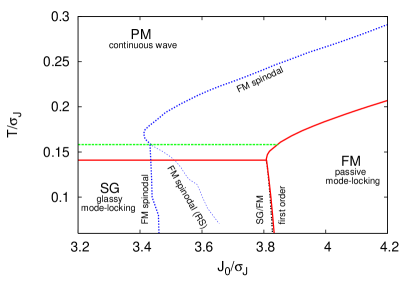
Figure 3: (Color online) Detail of the $J_{0},T$ phase diagram around the tricritical point. Full lines are thermodynamic transitions. Also the transition between the SG (1RSB) and the approximated RS solution for the FM phase is displayed (double-dotted line) showing no appreciable difference with the exact one. The dashed line represents the dynamic PM/SG transition. The dotted bold line represents the FM spinodal lines both inside the PM and the SG phases. The spinodal of the RS FM phase is shown as well (smaller dots).

Paramagnetic phase — For low ${\cal P}$ the only phase present is completely disordered: all order parameters are zero and we have a “paramagnet” (PM); for the random laser case this phase is expected to correspond to a noisy continuous wave emission, and all the mode-phases are uncorrelated. Actually, this phase exists for any degree of disorder and pumping, yet it becomes thermodynamically sub-dominant as ${\cal P}$ (or $\beta$) increases and, depending on the degree of disorder, the spin-glass or the ferromagnetic phases take over.
Glassy phase — For large disorder, as ${\cal P}$/$\beta$ grows, a discontinuous transition occurs from the PM to a spin-glass (SG) phase in which the phases $\phi$ are frozen but do not display any ordered pattern in space. First, along the line ${\cal P}_{d}=\sqrt{\bar{\beta}_{d}/R_{J}}$, in Fig. 1, or at $T/\sigma_{J}=1/\bar{\beta}_{d}=0.15447$ in Figs. 2, 3 (dashed lines) a dynamic transition occurs. Indeed, the lifetime of metastable states is infinite in the mean-field model and the dynamics gets stuck in the highest lying excited states. The thermodynamic state is, however, still PM. Fig. 3 displays a detail of the tricritical region where. There, besides thermodynamic transition lines, we also plot as dotted curves the lines at which the ferromagnetic phase first appears as metastable, i.e., the spinodal lines.

Figure 4: Complexity $\Sigma({\cal P})$ of the lowest lying glassy states in free energy between the values of the pumping rate corresponding to the dynamic and static transition from the PM to the SG phase at $R_{J}=0.5$.

Figure 5: Left: Complexity of the lowest lying glassy states in free energy $\Sigma({\cal P})$ between dynamic and static transition from the PM to the SG phase along $R_{J}=0.3,0.4$ and $0.5$ lines. The qualitative behavior is identical for any $R_{J}\gtrsim 0.3$. Right: $\Sigma$ vs. the effective temperature $T$ in $\sigma_{J}$ units.

Figure 6: $\Sigma(f)$ (left) and $\Sigma(m)$ (right) in the glassy phase at the static transition effective temperature, $T=0.14099$. This is the picture holding for any $R_{J}\gtrsim 0.3$.

Figure 7: $\Sigma(f)$ (left) and $\Sigma(m)$ (right) in the glassy phase at the static transition effective temperature, $T=0.15<T_{d}$. The lowest state free energy of metastable glassy states is denoted by $f_{1}$ (i.e., corresponding to $m=1$ in the right panel, see text). The free energy of maximum complexity is denoted by $f^{*}$, correspondingly $m^{*}$ in the right hand side plot.

In Fig. 4 we plot the complexity of the metastable glassy states of lowest free energy between the dynamic and the static transition. In the left panel of Fig. 5 $\Sigma({\cal P})$ is displayed for three different values of $R_{J}$; the threshold pumping for non-zero minimal complexity grows as the degree of disorder $R_{J}$ decreases, as well as the corresponding ${\cal P}$ range. In the right panel $\Sigma(T)$ is plotted and it is independent of $R_{J}$. In Figs. 6 and 7 we display two instances of the whole complexity curve both vs. $f$ and $m$ at $T=T_{s}$ and at a higher temperature $T<T_{d}$.
Across the full line ${\cal P}_{s}(R_{J})=\sqrt{\bar{\beta}_{s}/R_{J}}$, in Fig. 1 or, alternatively, across $T/\sigma_{J}=1/\bar{\beta}_{s}=0.14099$ in Fig. 2, a true thermodynamic phase transition from the continuous wave (paramagnetic) phase to the “glassy coherent light” (spin-glass) phase occurs. The order parameter $q_{1}$ (the Edwards-Anderson parameter $q_{\rm EA}$ Edwards and Anderson (1975)), discontinuously jumps at the transition from zero $q_{1}>q_{0}=0$, while $\tilde{m}=r_{0}=r_{1}=r_{d}=0$ (see Fig. VI, bottom panel). The SG phase exists for any value of $R_{J}$ and $\bar{\beta}>\bar{\beta}_{s}$.
In the stable SG phase, metastable states (with infinite lifetime) continue to exist so that the thermodynamic state is actually unreachable along a standard dynamics starting from random initial condition. In Fig. 9 we plot the typical behavior of the complexity versus the single state free energy at $T/\sigma_{J}=0.1$, qualitatively identical to the left panel of Fig. 6 displaying $\Sigma(f)$ at $T=T_{s}$.

Ferromagnetic phase — For weak disorder a random ferromagnetic (FM) phase turns out to dominate over both the SG and the PM phases. The transition PM/FM line is the standard passive ML threshold (see e.g. [Gordon and Fischer, 2002, 2003]) and it turns out to be first order in the Ehrenfest (i.e., thermodynamic) sense Leuzzi and Nieuwenhuizen (2007); Ehrenfest (1980). From Fig. 1 we see that it takes place at growing pumping rates ${\cal P}$ for increasing $R_{J}$ until it reaches the tricritical point with the SG phase. In the $(T,J_{0})$ plane it occurs at large - positive - $J_{0}$, cf. Fig.2
To precisely describe the FM phase in the 1RSB Ansatz we have to solve eleven coupled integral equations [Eqs. (51)-(55) and Eq. (59) ($\Sigma(m;\bm{Q}_{\rm sp}),\bm{\Lambda}_{\rm sp})=0$), cf. Eq. (61)]. In evaluating their solutions we have to consider that, in the region where the FM phase is thermodynamically dominant, both the PM and the SG solutions also satisfy the same set of equations. Besides, unfortunately, the basin of attraction of the latter two phases - in terms of initial conditions - is much broader than the FM one. Starting the iterative resolution from random initial conditions, determining the FM transition and spinodal lines becomes, thus, numerically demanding.
An approximation can be obtained by considering the Replica Symmetric (RS) solution for the FM phase (FM_rs). This reduces the number of independent parameters to seven ($q_{1}=q_{0}$, $r_{1}^{R,I}=r_{0}^{R,I}$, $r_{d}^{R,I}$ and $\tilde{m}^{R,I}$). The corresponding transition line is shown as a Figure 8: Discontinuity of the order parameters at the transition points for three values of $R_{J}$. Top Left panel: jump in $q_{0,1}$, at the PM/FM transition in ${\cal P}$ for small disorder, $R_{J}\simeq 0.1$; top right: discontinuities in $r_{0,1}$, ${\tilde{r}}$ and ${\tilde{m}}$ at the same transition. For such small $R_{J}$ the replica symmetry breaking is practically invisible: $q_{1}\simeq q_{0}$, $r_{1}\simeq r_{0}$ [to the precision of our computation, ${\cal O}(10^{-5})$]. Mid left panel (across tricritical region in Fig. 1: $q_{0,1}$ vs. ${\cal P}$ at $R_{J}\simeq 0.26$ where, increasing the pumping rate, first a PM/FM transition occurs followed by a FM/SG one. Mid right panel: $r_{0,1}$, $\tilde{r}$ and $\tilde{m}$ vs. ${\cal P}$ for the same interval. First order transition point are signaled by vertical lines. Left bottom panel: $q_{0,1}$ vs. ${\cal P}$ for large disorder, $R_{J}=0.4$ across the PM/SG random first order transition. Right bottom: $r_{0,1}$, $\tilde{r}$ and $\tilde{m}$ are always zero in the SG and in the PM phase. dashed-dotted line in Fig. 3, where, around the transition, we observe no practical difference with the exact SG/FM, even though the replica symmetry is clearly broken.

In Fig. VI we show the discontinuous behavior of the order parameters across various transitions. As disorder is small (top panel) one can observe that the RSB of the solution representing the passive mode-locking phase vanishes, at least for what concerns the limit of precision of our computation. As the degree of disorder takes values around the tricritical point the RSB is clearly visible (mid panel), both in the FM and in the SG phases. For increasing disorder the FM is absent ($R_{J}\gtrsim 0.263$) and at high pumping/low temperature only the glassy random laser phase remains.

Figure 9: Complexity vs. free energy curve is plotted in the SG phase (left) at $T/\sigma_{J}=0.1$ and in the FM phase (right).

We must necessarily implement the 1RSB Ansatz, though, to determine the not-vanishing extensive complexity which signals the presence of a large quantity of excited states with respect to ground states and study its behavior in $T$ and $R_{J}$. This, as anticipated, also implies the occurrence of a dynamic transition besides the thermodynamic one. In the phase diagrams, Figs. 1, 2, 3, this takes place between PM and SG, where the state structure always displays a non-trivial $\Sigma$, for any $\bar{\beta}>\bar{\beta}_{d}$. Whether an exclusively dynamic transition can occur as a precursor to the FM phase, as well, could not be directly established in the present work. Indeed, the region of expected dynamic transition lies beyond the spinodal FM line, already very difficult to obtain numerically because of the competition with the SG and PM solutions. However, the existence of a metastable FM phase (cf. spinodal line in Fig. 3) with an extensive complexity, cf. e.g., Figs. 9 and 10, might well correspond to an arrest of the dynamic relaxation towards equilibrium of the system.

Figure 10: Complexity curves of the FM phase at $R_{J}=3.54$ at temperatures between $T=0.082\sigma_{J}$ (right most) and $T=0.139\sigma_{J}$ (left most). Both the magnitude of the maximal complexity and the free energy interval in which $\Sigma(f)>0$ decrease. Notice that the equilibrium free energy decreases as temperature increases.

Figure 11: Top panel: free energy of the FM and SG phases vs. $R_{J}$ at $T=0.0785$. As the degree of disorder increases the system undergoes a first order phase transition from a ferromagnetic phase to a spin-glass. Mid panel: order parameters $r_{1},r_{0}$, $\tilde{r}$ and the magnetization $\tilde{m}$ are shown vs. $R_{J}$. Beyond the transition point their values drop to zero in the SG phase. Bottom panel: $q$ order parameters for the FM and the SG phase.

In the right inset of Fig. 9 we show, e.g., $\Sigma(f)$ in the FM phase at $(R_{J},{\cal P})=(0.28,5.92)$. This has to be compared with the SG complexity at the same temperature (left inset of Fig. 9) that is sensitively larger and does not depend on the $R_{J}$: the maximum complexity drops of about two orders of magnitude at the SG/FM transition, thus unveiling a corresponding high to low complexity transition.
In Fig. 11, at a relatively low temperature $T=0.0785$ we show the behavior of the 1RSB (equilibrium) free energy and order parameters across this SG (high complexity)/FM (low complexity) transition. The transition is first order in $R_{J}$.

VII Conclusion

We have reported on an extensive theoretical treatment of the thermodynamic and dynamic phases of nonlinear waves in a random systems. The approach allows to treat nonlinearity and an arbitrary degree of disorder on the same ground, and predict the existence of complex coherent phases detailed in a specific phase-diagram. The whole theoretical treatment is limited to the quenched-amplitude approximation, which allows to catch the basic phenomenology and to demonstrate the existence of phases with a not-vanishing complexity in a variety of physical systems, and specifically random lasers, finite temperature BEC and nonlinear optics. This approximation will be removed in future works, and novel exotic phases of light in nonlinear random system will be detailed.

Our theoretical work shows that the interplay of nonlinearity and disorder leads to the prediction of substantially innovative physical effects, which bridge the gap between fundamental mathematical models of statistical mechanics and nonlinear waves. This allows to identify frustration and complexity as the leading mechanisms for a coherent wave regime in nonlinear disordered systems. Natural extension of this work will be considering the quantum counterpart of the predicted transitions, and the analysis of out of equilibrium nonlinear waves dynamics.

Appendix A Replica computation of the thermodynamic properties

The replicated partition function of the system described by the Hamiltonian ${\cal H}[\{\phi_{j}\}]$, cf. Eq. (I.1), reads

$$Z^{n}_{J}=\int\prod_{a=1}^{n}\prod_{j=1}^{N}d\phi^{a}_{j}\exp\left[-\beta\sum_{a=1}^{n}{\cal H}[\{\phi_{j}^{a}\}]\right]$$ (63)

In order to compute the free energy of the system using the replica trick, cf. Eq. (39), Eq. (63) has to be averaged over the probability distribution of i.i.d. random bonds:

$$P(J)\equiv\sqrt{\frac{N^{3}}{2\pi\sigma_{J}^{2}}}\exp\left[-N^{3}\frac{(J-J_{0}/N^{3})^{2}}{2\sigma_{J}^{2}}\right]$$ (64)

Eq. (41), then reads

$${\overline{Z_{J}^{n}}}=\int{\cal D}\phi\exp\Biggl{\{}N\Biggl{[}\frac{\beta^{2}\sigma_{J}^{2}}{32}\sum_{a=1}^{n}\left(1+\left|\tilde{R}_{a}(\{\phi\})\right|^{4}\right)$$

$$\hskip 51.21504pt+\frac{\beta^{2}\sigma_{J}^{2}}{16}\sum_{a<b}\left(\left|Q_{ab}(\{\phi\})\right|^{4}+\left|R_{ab}(\{\phi\})\right|^{4}\right)$$

$$\hskip 119.50148pt+\frac{\beta J_{0}}{8}\sum_{a=1}^{n}\left|M_{a}(\{\phi\})\right|^{4}\Biggr{]}\Biggr{\}}$$

with

$${\cal D}\phi\equiv\prod_{a=1}^{n}\prod_{j=1}^{N}d\phi^{a}_{j}$$ (66)

and

$$Q_{ab}(\{\phi\})\equiv\frac{1}{N}\sum_{j=1}^{N}e^{\imath(\phi_{j}^{a}-\phi_{j}^{b})};\quad M_{a}(\{\phi\})\equiv\frac{1}{N}\sum_{j=1}^{N}e^{\imath\phi_{j}^{a}}$$

(67)

$$R_{ab}(\{\phi\})\equiv\frac{1}{N}\sum_{j=1}^{N}e^{\imath(\phi_{j}^{a}+\phi_{j}^{b})};\quad\tilde{R}_{a}(\{\phi\})\equiv\frac{1}{N}\sum_{j=1}^{N}e^{2\imath\phi_{j}^{a}}$$

(68)

where we used the Euler’s formula to represent the cosine and introduced abbreviations for the quantities Eqs. (67)-(68). We notice that the matrix $Q_{ab}$ is Hermitian. A further step is to introduce extra parameters - that will eventually result as the order parameters identifying the various phases of the system - by means of the following identities:

$$1=\prod_{a<b}^{1,n}N\int dq_{ab}\delta\left[N\left(Q_{ab}(\{\phi\})-q_{ab}\right)\right]$$ (69)

$$1=\prod_{a<b}^{1,n}N\int dr_{ab}\delta\left[N\left(R_{ab}(\{\phi\})-r_{ab}\right)\right]$$ (70)

$$1=\prod_{a=1}^{n}N\int d\tilde{r}_{a}\delta\left[N\left(\tilde{R}_{a}(\{\phi\})-\tilde{r}_{a}\right)\right]$$ (71)

$$1=\prod_{a=1}^{n}N\int d\tilde{m}_{a}\delta\left[N\left(M_{a}(\{\phi\})-\tilde{m}_{a}\right)\right]$$ (72)

$$\delta\left[N\left(Q_{ab}(\{\phi\})-q_{ab}\right)\right]=\int\frac{d\lambda_{ab}}{2\pi}e^{\Re\left[\bar{\lambda}_{ab}N\left(Q_{ab}(\{\phi\})-q_{ab}\right)\right]}$$

(73)

$$\delta\left[N\left(R_{ab}(\{\phi\})-r_{ab}\right)\right]=\int\frac{d\mu_{ab}}{2\pi}e^{\Re\left[\bar{\mu}_{ab}N\left(R_{ab}(\{\phi\})-r_{ab}\right)\right]}$$

(74)

$$\delta\left[N\left(\tilde{R}_{a}(\{\phi\})-\tilde{r}_{a}\right)\right]=\int\frac{d\tilde{\mu}_{a}}{2\pi}e^{\Re\left[{\bar{\tilde{\mu}}}_{a}N\left(\tilde{R}_{a}(\{\phi\})-\tilde{r}_{a}\right)\right]}$$

(75)

$$\delta\left[N\left(M_{a}(\{\phi\})-\tilde{m}_{a}\right)\right]=\int\frac{d\nu_{a}}{2\pi}e^{\Re\left[\bar{\nu}_{ab}N\left(M_{a}(\{\phi\})-\tilde{m}_{a}\right)\right]}$$

The two-index auxiliary variables $q_{ab},r_{ab}$, defined for distinct couples of replicas $a$ and $b$, with $a<b$, will be considered in the following as elements of symmetric matrices [cf. Eqs. (88) and (114) ], i.e., $q_{ab}=q_{ba}$ and $r_{ab}=r_{ba}$. In particular, since $Q_{ab}(\phi)=\bar{Q}_{ba}(\phi)$, Eq. (69) implies that $q_{ab}=\bar{q}_{ab}$ are real valued.
Denoting for shortness the sets of parameters by the “vectors” $\mathbf{Q}=\{q,r,\tilde{r},\tilde{m}\}$ and $\mathbf{\Lambda}=\{\lambda,\mu,\tilde{\mu},\nu\}$, this leads to

$${\overline{Z_{J}^{n}}}=\int{\cal D}\mathbf{Q}~{}{\cal D}\mathbf{\Lambda}~{}e^{-N~{}n~{}G\left[\mathbf{Q},\mathbf{\Lambda}\right]}$$ (76)

$$n~{}G\left[\mathbf{Q},\mathbf{\Lambda}\right]=n~{}A\left[\mathbf{Q},\mathbf{\Lambda}\right]+\log Z_{\phi}\left[\mathbf{\Lambda}\right]$$

$$n~{}A\left[\mathbf{Q},\mathbf{\Lambda}\right]\equiv-\frac{\beta^{2}\sigma_{J}^{2}}{32}\sum_{a=1}^{n}\Bigl{(}1+\left|\tilde{r}_{a}\right|^{4}\Bigr{)}-\frac{\beta J_{0}}{8}\sum_{a=1}^{n}\left|\tilde{m}_{a}\right|^{4}$$

$$\hskip 14.22636pt-\frac{\beta^{2}\sigma_{J}^{2}}{16}\sum_{a<b}^{1,n}\Bigl{(}\left|q_{ab}\right|^{4}+\left|r_{ab}\right|^{4}\Bigr{)}-\sum_{a<b}^{1,n}\Re\bigl{[}q_{ab}\bar{\lambda}_{ab}+r_{ab}\bar{\mu}_{ab}\bigr{]}$$

$$\hskip 28.45274pt-\sum_{a=1}^{n}\Re\bigl{[}\tilde{r}_{a}{\bar{\tilde{\mu}}}_{a}+\tilde{m}_{a}\nu_{a}\bigr{]}$$ (77)

$$Z_{\phi}\left[\mathbf{\Lambda}\right]\equiv\int\prod_{a=1}^{n}d\phi_{a}e^{-\beta{\cal H}_{\rm eff}[\{\phi\};\mathbf{\Lambda}]}$$ (78)

$$-\beta{\cal H}_{\rm eff}[\{\phi\};\mathbf{\Lambda}]\equiv\sum_{a<b}^{1,n}\Re\bigl{[}e^{\imath(\phi_{a}-\phi_{b})}\bar{\lambda}_{ab}+e^{\imath(\phi_{a}+\phi_{b})}\bar{\mu}_{ab}\bigr{]}$$

$$\hskip 56.9055pt+\sum_{a=1}^{n}\Re\bigl{[}e^{2\imath\phi_{a}}{\bar{\tilde{\mu}}}_{a}+e^{\imath\phi_{a}}\bar{\nu}_{a}\bigr{]}$$ (79)

with

$${\cal D}\mathbf{Q}\equiv\prod_{a<b}^{1,n}N^{2}dq_{ab}dr_{ab}\times\prod_{a=1}^{n}N^{2}d\tilde{r}_{a}d\tilde{m}_{a}$$

$${\cal D}\mathbf{\Lambda}\equiv\prod_{a<b}^{1,n}\frac{d\lambda_{ab}}{2\pi}\frac{d\mu_{ab}}{2\pi}\times\prod_{a=1}^{n}\frac{d\tilde{\mu}_{a}}{2\pi}\frac{d\nu_{a}}{2\pi}$$

The average replicated partition function integral can be estimated by the saddle point method for large $N$, i.e., by approximating

$$\int{\cal D}[\mathbf{X}]~{}e^{N~{}F[\mathbf{X}]}\simeq e^{N~{}F[\mathbf{X}_{\rm sp}]}$$

$$\frac{\partial F}{\partial X_{j}}\bigr{|}_{\mathbf{X}=\mathbf{X}_{\rm sp}}=0\quad\forall~{}j=1,\ldots,\mbox{\# parameters}$$

Denoting by $\langle\ldots\rangle_{\rm eff}$ the average over the measure $e^{-\beta{\cal H}_{\rm eff}}$, the saddle point equations are:

$$q_{ab} = \langle e^{\imath(\phi_{a}-\phi_{b})}\rangle_{\rm eff};\quad\lambda_{ab}=\frac{\beta^{2}\sigma_{J}^{2}}{4}\left|q_{ab}\right|^{2}q_{ab}\ \ \$$ (80)

$$r_{ab} = \langle e^{\imath(\phi_{a}+\phi_{b})}\rangle_{\rm eff};\quad\mu_{ab}=\frac{\beta^{2}\sigma_{J}^{2}}{4}\left|r_{ab}\right|^{2}r_{ab}\ \ \$$

$$\forall~{}a,b=1,\ldots,n;~{}a<b$$

$$\tilde{r}_{a\ } = \langle e^{2\imath\phi_{a}}\rangle_{\rm eff};\qquad\quad\tilde{\mu}_{a}=\frac{\beta^{2}\sigma_{J}^{2}}{8}\left|\tilde{r}_{a}\right|^{2}\tilde{r}_{a}$$ (82)

$$\tilde{m}_{a} = \langle e^{\imath\phi_{a}}\rangle_{\rm eff};\qquad\quad\ \nu_{a}=\frac{\beta J_{0}}{2}\left|\tilde{m}_{a}\right|^{2}\tilde{m}_{a}$$

$$\forall~{}a=1,\ldots,n$$

The diagonal values of the overlap matrices are set to zero. Eventually, according to Eq. (39), one has

$$\beta\Phi=-\frac{1}{N}\lim_{n\to 0}\frac{e^{-nNG\left[\mathbf{Q}_{\rm sp},\mathbf{\Lambda}_{\rm sp}\right]}-1}{n}=\lim_{n\to 0}G\left[\mathbf{Q}_{\rm sp},\mathbf{\Lambda}_{\rm sp}\right]$$ (84)

The parameters with a single replica index turn out not to depend on the specific replica. Indeed, Eqs. (82)-(A) might in principle be obtained by perturbing the original Hamiltonian with a small field coupled to a local function of the planar, XY, spins $S=e^{\imath\phi}$, independently from the possible introduction of replicas.

If the perturbation is $-k\sum_{j=1}^{N}S_{j}^{2}$ we obtain

$$\tilde{r}_{d}=-\frac{1}{N}\frac{\partial{\overline{\log Z_{J}}}}{\partial k}=\frac{1}{N}\sum_{j=1}^{N}{\overline{S_{j}^{2}}}\,\to\,{\overline{\langle S\rangle}}\quad\mbox{(as $N\to\infty$)}$$

(85)

that is valid for any replica, and, therefore independent from any replica index: $\tilde{r}_{d}=\tilde{r}_{a}$, $\forall a=1,\ldots,n$. In the replica formalism, the same quantity can equivalently be written, as

$$\tilde{r}_{d}=-\lim_{n\to 0}\frac{1}{nN}\frac{\partial{\overline{Z_{J}^{n}}}}{\partial k}=\lim_{n\to 0}\frac{1}{n}\sum_{a=1}^{n}\tilde{r}_{a}$$

and this trivially leads to the identification

$$\tilde{r}_{a}=\lim_{n\to 0}\frac{1}{n}\sum_{a=1}^{n}\tilde{r}_{a}=\tilde{r}_{d}$$ (86)

Similarly, perturbing Eq. (I.1) with $-h\sum_{j=1}^{N}S_{j}$ we get

$$\tilde{m} = -\frac{1}{N}\frac{\partial{\overline{\log Z_{J}}}}{\partial h}=\frac{1}{N}\sum_{j=1}^{N}{\overline{S_{j}}}$$ (87)

$$\tilde{m} = -\lim_{n\to 0}\frac{1}{nN}\frac{\partial{\overline{Z_{J}^{n}}}}{\partial h}=\lim_{n\to 0}\frac{1}{n}\sum_{a=1}^{n}\tilde{m}_{a}$$

Though no external ad hoc perturbation can be applied to the Hamiltonian Eq. (79) to reproduce two indices quantities, the same symmetry should apply, since all replicas of the original problem were introduced in the same way: the system is symmetric under replica exchange. This is called the replica symmetric (RS) Ansatz.

$$q_{ab}=q~{}~{}~{}\forall a\neq b~{};\qquad r_{ab}=r~{}~{}~{}\forall a\neq b$$ (88)

A.1 Replica Symmetric Ansatz

In this Ansatz Eqs. (78,79) become

$$Z_{\phi}^{\rm RS}=\int\prod_{a=1}^{n}d\phi_{a}e^{-\beta{\cal H}_{\rm eff}[\{\phi_{a}\}]}$$ (89)

$$\beta{\cal H}_{\rm eff}=\frac{\lambda^{R}}{2}\left(n-\left|\sum_{a=1}^{n}e^{\imath\phi_{a}}\right|^{2}\right)$$ (90)

$$-\Re\left[\frac{\bar{\mu}}{2}\left(\sum_{a=1}^{n}e^{\imath\phi_{a}}\right)^{2}+\left(\bar{\tilde{\mu}}-\frac{\bar{\mu}}{2}\right)\sum_{a=1}^{n}e^{2\imath\phi}+\bar{\nu}\sum_{a=1}^{n}e^{\imath\phi}\right]$$

The second term in the rhs can be rewritten as

$$\Re\left[\frac{\bar{\mu}}{2}\left(\sum_{a=1}^{n}e^{\imath\phi_{a}}\right)^{2}\right]=\Re\left[\frac{\mu}{2}\left(\sum_{a=1}^{n}e^{-\imath\phi_{a}}\right)^{2}\right]$$ (91)

$$=\Re\left[\frac{1}{4}\left(\sqrt{\bar{\mu}}\sum_{a=1}^{n}e^{\imath\phi_{a}}+\sqrt{\mu}\sum_{a=1}^{n}e^{-\imath\phi_{a}}\right)^{2}\right]$$

$$\ \ \ -\frac{|\mu|}{2}\left|\sum_{a=1}^{n}e^{\imath\phi_{a}}\right|^{2}$$

The squared terms in the exponent of the integrand can be linearized by using

$$e^{|w|^{2}/2}=\int\frac{d\zeta^{R}d\zeta^{I}}{2\pi}e^{-|\zeta|^{2}/2}e^{\Re(\bar{\zeta}w)}$$ (92)

$$e^{w_{R}^{2}/2}=\int\frac{dx}{\sqrt{2\pi}}e^{-x^{2}/2}e^{xw_{R}}$$ (93)

thus yielding

$$Z_{\phi}^{\rm RS}=\int{\cal D}p(x){\cal D}p(\zeta^{R}){\cal D}p(\zeta^{I})\biggl{[}\int_{0}^{2\pi}d\phi e^{{\cal L}(\phi;x,\zeta)}\biggr{]}^{n}$$ (94)

$${\cal L}(\phi;x,\zeta)\equiv\Re\biggl{[}e^{\imath\phi}\left(\bar{\zeta}\sqrt{\lambda-|\mu|}+x{\sqrt{2\bar{\mu}}}+\bar{\nu}\right)$$ (95)

$$\hskip 113.81102pt+e^{2\imath\phi}\left({\bar{\tilde{\mu}}}-\frac{\bar{\mu}}{2}\right)\biggr{]}$$

$${\cal D}p(w)=\frac{dw}{\sqrt{2\pi}}e^{-w^{2}/2}$$ (96)

The replicated free energy eventually reads:

$$\beta\Phi=-\frac{\beta^{2}\sigma_{J}^{2}}{32}\left[1-|q|^{4}-|r|^{4}+|\tilde{r}|^{4}\right]$$ (97)

$$-\frac{\beta J_{0}}{8}|\tilde{m}|^{4}+\frac{\lambda^{R}}{2}(1-q^{R})-\frac{1}{2}\Re\left[\bar{\mu}r-2{\bar{\tilde{\mu}}}{\tilde{r}}-2{\bar{\nu}}\tilde{m}\right]$$

$$-\int{\cal D}p(x){\cal D}p(\zeta^{R}){\cal D}p(\zeta^{I})\log\int_{0}^{2\pi}d\phi~{}e^{{\cal L}(\phi;x,\zeta)}$$

Deriving w.r.t. to $Q$’s parameter we obtain the specification of Eqs. (80-A) for the replica overlap parameters $q$, $r$ and for $\tilde{r}$ and $\tilde{m}$

$$\lambda = \frac{\beta^{2}\sigma_{J}^{2}}{4}q^{3}\ \ \$$ (98)

$$\mu = \frac{\beta^{2}\sigma_{J}^{2}}{4}\left|r\right|^{2}r\ \ \$$ (99)

$$\tilde{\mu} = \frac{\beta^{2}\sigma_{J}^{2}}{8}\left|\tilde{r}\right|^{2}\tilde{r}$$

$$\nu = \frac{\beta J_{0}}{2}\left|\tilde{m}\right|^{2}\tilde{m}$$

Taking the derivative of $\beta\Phi$ in Eq. (97) w.r.t. $\tilde{\mu}$ and $\nu$ we obtain

$$\tilde{r}_{d} = \langle\langle e^{2\imath\phi}\rangle_{\cal L}\rangle_{x,\zeta}$$ (100)

$$\tilde{m} = \langle\langle e^{\imath\phi}\rangle_{\cal L}\rangle_{x,\zeta}$$ (101)

where we define

$$\langle\ldots\rangle_{\cal L}\equiv\frac{\int_{0}^{2\pi}d\phi\ldots~{}e^{{\cal L}(\phi;x,\zeta)}}{\int_{0}^{2\pi}d\phi~{}e^{{\cal L}(\phi;x,\zeta)}}$$ (102)

Deriving $G$ w.r.t. $\lambda$ and $\mu$ and equating to zero we obtain

$$q^{R} = \left<c_{\cal L}^{2}+s_{\cal L}^{2}\right>_{x,\zeta}$$ (103)

$$r = \left<c_{\cal L}^{2}-s_{\cal L}^{2}+2\imath~{}c_{\cal L}s_{\cal L}\right>_{x,\zeta}$$

$$c_{\cal L}\equiv\langle\cos\phi\rangle_{\cal L}\qquad s_{\cal L}\equiv\langle\sin\phi\rangle_{\cal L}$$

after having integrated by part in the Gaussian measures. To help the non-expert reader to easily derive the self-consistency equations we exemplify the calculation of Eq. (80).

$$2\frac{\partial G}{\partial\lambda^{R}}=0=1-q^{R}$$ (105)

$$\ \ \ -\left<\left(\zeta^{R}c_{\cal L}+\zeta^{I}s_{\cal L}\right)\right>_{x,\zeta}/\sqrt{\lambda^{R}-|\mu|}$$

The latter term can be simplified by integrating by part

$$\int_{-\infty}^{\infty}{\cal D}p(y)~{}y~{}F(y)=\int_{-\infty}^{\infty}{\cal D}p(y)~{}\frac{\partial F(y)}{\partial y}$$ (106)

with $y=\zeta^{R},\zeta^{I}$ in Eq. (A.1), yielding

$$\left<\zeta^{R}c_{\cal L}+\zeta^{I}s_{\cal L}\right>_{x,\zeta}=\sqrt{\lambda^{R}-|\mu|}\times$$ (107)

$$\quad\left<\cos^{2}\phi-c_{\cal L}^{2}+\sin^{2}\phi-s_{\cal L}^{2}\right>_{x,\zeta}$$

The self-consistency equation can thus be rewritten as, cf. Eq. (51),

$$1-q^{R}=1-\left<c_{\cal L}^{2}+s_{\cal L}^{2}\right>_{x,\zeta}$$

$$q^{R}=\left<c_{\cal L}^{2}\right>_{x,\zeta}+\left<s_{\cal L}^{2}\right>_{x,\zeta}$$

We recall that since $q_{ab}$ is real, and so is $\lambda_{ab}$, cf. Eq. (80), in the RS Ansatz the equations $q^{I}=\lambda^{I}=0$.

Before deriving Eq. (A.1), we rewrite the part of Eq. (95) involving the integrating variable $x$ as:

$$\Re\biggl{[}e^{\imath\phi}x{\sqrt{2\bar{\mu}}}\biggr{]}=$$ (108)

$$\qquad x\sqrt{|\mu|}\Biggl{(}\cos\phi\sqrt{1+\frac{\mu^{R}}{|\mu|}}+\sin\phi\sqrt{1-\frac{\mu^{R}}{|\mu|}}\Biggr{)}$$

In determining the above expression one can use, e.g., the trigonometric law of tangents to yield

$$\frac{1}{2}\arctan\frac{\mu^{I}}{\mu^{R}}=\arctan\sqrt{\frac{1-\mu^{R}/|\mu|}{1+\mu^{R}/|\mu|}}$$ (109)

and the relationships between trigonometric and inverse trigonometric functions:

$$\sin[\arctan(\theta)]=\frac{\theta}{\sqrt{1+\theta^{2}}}$$

$$\cos[\arctan(\theta)]=\frac{1}{\sqrt{1+\theta^{2}}}$$

Using Eq. (A.1), together with Eqs. (100) and (103), we have:

$$2\frac{\partial G}{\partial\mu^{R}}=0=r_{d}^{R}-r^{R}+\frac{\mu^{R}}{|\mu|}(1-q)$$ (110)

$$\ \ \ -\left<x\left(c_{\cal L}\sqrt{1+\frac{\mu^{R}}{|\mu|}}+s_{\cal L}\sqrt{1-\frac{\mu^{R}}{|\mu|}}\right)\right>_{x,\zeta}/\sqrt{|\mu|}$$

Integrating by part with Eq. (106), $y=x$, we find

$$\left<x\left(c_{\cal L}\sqrt{1+\frac{\mu^{R}}{|\mu|}}+s_{\cal L}\sqrt{1-\frac{\mu^{R}}{|\mu|}}\right)\right>_{x,\zeta}$$ (111)

$$\hskip 56.9055pt=\sqrt{|\mu|}\Biggl{<}\biggl{[}\langle\cos 2\phi\rangle_{\cal L}-c_{\cal L}^{2}+s_{\cal L}^{2}$$

$$\hskip 110.96556pt+\frac{\mu^{R}}{|\mu|}\left(1-c_{\cal L}^{2}-s_{\cal L}^{2}\right)\biggr{]}\Biggr{>}_{x,\zeta}$$

and eventually one obtains the real part of Eq. (A.1). The imaginary part of the self-consistency equation for $r$ is analogously determined from $\frac{\partial G}{\partial\mu^{I}}=0$.

Above a given critical temperature (depending on $J_{0}$) the solution to Eqs. (100,101,103,A.1) is paramagnetic, i.e., $q=r=\tilde{m}=\tilde{r}=0$ and the free energy is

$$\beta\Phi_{PM}=-\frac{\bar{\beta}^{2}}{32}-\log 2\pi$$ (112)

Below $T_{c}(J_{0})$, depending on the value of $J_{0}$ the solution can either be ferromagnetic $\tilde{m}\neq 0$ or spin-glass $\tilde{m}=0$. The latter solutions are, however, not stable against fluctuations in the space of replica overlaps and, thus, we have to try an Ansatz different from Eq. (88) to provide a self-consistent thermodynamics.

A.2 One step of Replica Symmetry Breaking

In order to obtain a thermodynamically consistent result the symmetry cannot be conserved. We are in presence of a spontaneous Replica Symmetry Breaking. The way to break the symmetry must be a-priori hypothesized, since there has been found, so far, no way to deduce it. The correct way to express the elements of the overlap matrices is called Parisi Ansatz Parisi (1979, 1980) and, depending on the kind of system, can consist of one or more RSB’s. According to what happens in other spin models with $p$-body quenched random interactions ($p$ being larger than $2$), the right Ansatz for the matrices of our model is the one-step RSB, that is, we have a $n\times n$ matrix divided in square blocks of $m\times m$ elements

$$q_{ab}=q_{1};\quad r_{ab}=r_{1}\ \ \ \mbox{if}~{}I\left(\frac{a}{m}\right)=I\left(\frac{b}{m}\right)$$ (113)

$$q_{ab}=q_{0};\quad r_{ab}=r_{0}\ \ \ \mbox{if}~{}I\left(\frac{a}{m}\right)\neq I\left(\frac{b}{m}\right)$$ (114)

For instance, for $n=6$ and $m=3$.

$q_{\left(\alpha\beta\right)}=\left(\begin{array}[]{clrrrr}0&q_{1}&q_{1}&q_{0}&q_{0}&q_{0}\\ q_{1}&0&q_{1}&q_{0}&q_{0}&q_{0}\\ q_{1}&q_{1}&0&q_{0}&q_{0}&q_{0}\\ q_{0}&q_{0}&q_{0}&0&q_{1}&q_{1}\\ q_{0}&q_{0}&q_{0}&q_{1}&0&q_{1}\\ q_{0}&q_{0}&q_{0}&q_{1}&q_{1}&0\end{array}\right)$

The one replica index observables are instead still RS, as exemplified in Eqs. (85-87). Now, let us write the ”vectorial” replica index

$$a\to\mathbf{a}=(a_{1},a_{2})$$

$$\phi_{a}\to\phi_{\mathbf{a}}=\phi_{a_{1},a_{2}}$$

$$\sum_{a=1}^{n}O_{a}=\sum_{a_{1}=1}^{n/m}\sum_{a_{2}=1}^{m}O_{a_{1}a_{2}}$$

Take a 1RSB matrix $K_{ab}$ and two replicated observables $g_{a}$ and $h_{a}$. The following expressions hold for the sum of a generic product

$$2\sum_{a<b}K_{ab}g_{a}h_{b}=K_{ab}g_{a}h_{b}$$

$$= K_{1}\sum_{a_{1}=1}^{n/m}\sum_{a_{2}\neq b_{2}}^{1,m}g_{a_{1}a_{2}}h_{a_{1}b_{2}}+K_{0}\sum_{a_{1}\neq b_{1}}^{1,n/m}\sum_{a_{2}b_{2}}^{1,m}g_{a_{1}a_{2}}h_{b_{1}b_{2}}$$

$$= K_{1}\sum_{a_{1}=1}^{n/m}\sum_{a_{2},b_{2}}^{1,m}g_{a_{1}a_{2}}h_{a_{1}b_{2}}-K_{1}\sum_{a_{1}=1}^{n/m}\sum_{a_{2}=1}^{m}g_{a_{1}a_{2}}h_{a_{1}a_{2}}$$

$$+K_{0}\sum_{a_{1},b_{1}}^{1,n/m}\sum_{a_{2},b_{2}}^{1,m}g_{a_{1}a_{2}}h_{b_{1}b_{2}}-K_{0}\sum_{a_{1}=1}^{n/m}\sum_{a_{2},b_{2}}^{1,m}g_{a_{1}a_{2}}h_{a_{1}b_{2}}$$

If we take $g=\bar{h}$

$$2\sum_{a<b}K_{ab}|g_{a}|^{2} = (K_{1}-K_{0})\sum_{a_{1}=1}^{n/m}\left|\sum_{a_{2}=1}^{m}g_{a_{1}a_{2}}\right|^{2}$$ (116)

$$-K_{1}\sum_{a=1}^{n}\left|g_{a}\right|^{2}+K_{0}\left|\sum_{a=1}^{n}g_{a}\right|^{2}$$

If we take $g=h$

$$2\sum_{a<b}K_{ab}|g_{a}|^{2} = (K_{1}-K_{0})\sum_{a_{1}=1}^{n/m}\left(\sum_{a_{2}=1}^{m}g_{a_{1}a_{2}}\right)^{2}$$ (117)

$$-K_{1}\sum_{a=1}^{n}\left(g_{a}\right)^{2}+K_{0}\left(\sum_{a=1}^{n}g_{a}\right)^{2}$$

Substituting into Eqs. (78,79) both Eq. (116) - with $K=\bar{\lambda}$ and $g=\bar{h}=e^{\imath\phi}$ - and Eq. (117) - with $K=\bar{\mu}$ and $g=h=e^{\imath\phi}$ - one obtains

$$Z_{\phi}^{1RSB} = \int\prod_{a_{1}=1}^{n/m}\prod_{a_{2}=1}^{m}e^{-\beta{\cal H}_{\rm eff}[\{\phi_{a_{1}a_{2}}\}}]$$ (118)

$$\beta{\cal H}_{\rm eff} = \Re\Bigl{[}-\frac{\Delta\bar{\lambda}}{2}\sum_{a_{1}=1}^{n/m}\left|\sum_{a_{2}=1}^{m}e^{\imath\phi_{a_{1}a_{2}}}\right|^{2}$$

$$\qquad-n\frac{\bar{\lambda}_{1}}{2}+\frac{\bar{\lambda}_{0}}{2}\left|\sum_{a=1}^{n}e^{\imath\phi_{a}}\right|^{2}$$

$$\qquad+\frac{\Delta\bar{\mu}}{2}\sum_{a_{1}=1}^{n/m}\left(\sum_{a_{2}=1}^{m}e^{\imath\phi_{a_{1}a_{2}}}\right)^{2}$$

$$\qquad-\frac{\bar{\mu}_{1}}{2}\sum_{a=1}^{n}e^{2\imath\phi}+\frac{\bar{\mu}_{0}}{2}\left(\sum_{a=1}^{n}e^{\imath\phi_{a}}\right)^{2}$$

$$\qquad\quad+{\bar{\tilde{\mu}}}\sum_{a=1}^{n}e^{2\imath\phi}+\bar{\nu}\sum_{a=1}^{n}e^{\imath\phi}\Bigr{]}$$

$$\Delta\bar{\lambda}=\bar{\lambda}_{1}-\bar{\lambda}_{0}\qquad\Delta\bar{\mu}=\bar{\mu}_{1}-\bar{\mu}_{0}$$

Using the identities

$$\Re[(ab)^{2}]=\Re[(\bar{a}\bar{b})^{2}]=\Re\left[\frac{(ab+\bar{a}\bar{b})^{2}}{2}-|a||b|\right]$$ (120)

$$e^{A_{R}|g|^{2}/2}=\int\frac{d\zeta_{R}d\zeta_{I}}{2\pi}e^{-|\zeta|^{2}/2}e^{\Re[\bar{\zeta}\sqrt{A_{R}}g]}$$ (121)

$$e^{\Re[A~{}g^{2}]/2}=\int_{-\infty}^{\infty}\frac{dx}{\sqrt{2\pi}}e^{-x^{2}/2}e^{x\Re[\sqrt{A}g]}$$ (122)

where $A$ is complex and $A_{R}$ is real, we can linearize the dependence on $e^{\imath\phi}$ in the partition function Eq. (118) using Gaussian integral expressions:

$$\Re\left[\frac{\bar{\lambda}_{0}}{2}\left|\sum_{a=1}^{n}e^{\imath\phi_{a}}\right|^{2}+\frac{\bar{\mu}_{0}}{2}\left(\sum_{a=1}^{n}e^{\imath\phi_{a}}\right)^{2}\right]$$ (123)

$$=\log\int{\cal D}[\mathbf{0}]\exp\Re\Bigl{[}\bar{\zeta}_{0}\sqrt{\lambda_{0}^{R}-|\mu_{0}|}\sum_{a=1}^{n}e^{\imath\phi_{a}}$$

$$+\frac{x_{0}}{\sqrt{2}}\left(\sqrt{\bar{\mu}_{0}}\sum_{a=1}^{n}e^{\imath\phi_{a}}+\sqrt{\mu_{0}}\sum_{a=1}^{n}e^{-\imath\phi_{a}}\right)\Bigr{]}$$

$$\Re\left[\frac{\Delta\bar{\lambda}}{2}\left|\sum_{a_{2}=1}^{m}e^{\imath\phi_{a_{1}a_{2}}}\right|^{2}+\frac{\Delta\bar{\mu}}{2}\left(\sum_{a_{2}=1}^{m}e^{\imath\phi_{a_{1}a_{2}}}\right)^{2}\right]$$ (124)

$$=\log\int{\cal D}[\mathbf{1}]\exp\Re\Bigl{[}\bar{\zeta}_{1}\sqrt{\Delta\lambda^{R}-|\Delta\mu|}\sum_{a_{2}=1}^{m}e^{\imath\phi_{a_{1}a_{2}}}$$

$$+\frac{x_{1}}{\sqrt{2}}\Bigl{(}\sqrt{\Delta\bar{\mu}}\sum_{a_{2}=1}^{m}e^{\imath\phi_{a_{1}a_{2}}}+\sqrt{\Delta\mu}\sum_{a_{2}=1}^{m}e^{-\imath\phi_{a_{1}a_{2}}}\Bigr{)}\Bigr{]}$$

where we defined the Gaussian measures:

$${\cal D}p(\zeta_{k}^{R,I})=\frac{d\zeta_{k}^{R,I}}{\sqrt{2\pi}}e^{-\left(\zeta_{k}^{R,I}\right)^{2}/2}$$ (125)

$${\cal D}p(x_{k})=\frac{dx_{k}}{\sqrt{2\pi}}e^{-x_{k}^{2}/2}$$ (126)

$${\cal D}[\mathbf{k}]={\cal D}p(\zeta_{k}^{R}){\cal D}p(\zeta_{k}^{I}){\cal D}p(x_{k})$$ (127)

Eq. (118) becomes

$$Z_{\phi}^{1RSB}=e^{-n\lambda_{1}^{R}/2}\times$$ (128)

$$\qquad\int{\cal D}[\mathbf{0}]\prod_{a_{1}=1}^{n/m}\Bigl{\{}\int{\cal D}[\mathbf{1}]\int{\cal D}\phi\prod_{a_{2}=1}^{m}e^{{\cal L}(\phi_{a_{1}a_{2}};\mathbf{0},\mathbf{1})}\Bigr{\}}$$

$${\cal L}(\psi;\mathbf{0},\mathbf{1})\equiv\Re\Bigl{[}e^{\imath\psi}\Bigl{(}\bar{\zeta}_{1}\sqrt{\Delta\lambda^{R}-|\Delta\mu|}$$ (129)

$$+\bar{\zeta}_{0}\sqrt{\lambda_{0}^{R}-|\mu_{0}|}+2x_{1}\sqrt{\frac{\Delta\bar{\mu}}{2}}+2x_{0}\sqrt{\frac{\bar{\mu}_{0}}{2}}+\bar{\nu}\Bigr{)}$$

$$\hskip 113.81102pt+e^{2\imath\psi}\left({\bar{\tilde{\mu}}}-\frac{\bar{\mu}_{1}}{2}\right)\Bigr{]}$$

cf. Eq. (46). In the $n\to 0$ limit the ’phase contribution’ to the replicated free energy is:

$$-\lim_{n\to 0}\frac{1}{n}\log Z_{\phi}^{1RSB}=\frac{\lambda_{1}^{R}}{2}$$ (130)

$$\qquad-\frac{1}{m}\int{\cal D}[\mathbf{0}]\log\int{\cal D}[\mathbf{1}]\left[\int d\phi~{}e^{{\cal L}(\phi;\mathbf{0},\mathbf{1})}\right]^{m}$$

and the free energy is

$$\beta\Phi=\lim_{n\to 0}G_{\rm 1RSB}[\mathbf{Q}_{\rm sp};\mathbf{\Lambda}_{\rm sp}]$$ (131)

$$\ \ =-\frac{\beta^{2}\sigma_{J}^{2}}{32}\Bigl{[}1-(1-m)\left(|q_{1}|^{4}+|r_{1}|^{4}\right)$$

$$\quad-m\left(|q_{0}|^{4}+|r_{0}|^{4}\right)+|\tilde{r}|^{4}\Bigr{]}$$

$$\quad-\frac{1}{2}\Re\Bigl{[}(1-m)(\bar{\lambda}_{1}q_{1}+\bar{\mu}_{1}r_{1})+m(\bar{\lambda}_{0}q_{0}+\bar{\mu}_{0}r_{0})\Bigr{]}$$

$$\quad-\frac{\beta J_{0}}{8}|\tilde{m}|^{4}+\Re\Bigl{[}{\bar{\tilde{\mu}}}\tilde{r}+\bar{\nu}\tilde{m}\Bigr{]}-\lim_{n\to 0}\frac{1}{n}\log Z^{\rm 1RSB}_{\phi}$$

Saddle point equations. Deriving $G/n$ with respect to the parameters we obtain the twelve self-consistency equations determining the order parameter values at given external pumping intensity and amount of disorder.

• Deriving w.r.t. to $Q$’s parameter we obtain the specification of Eqs. (80-A) for each 1RSB replica matrix sector and for $\tilde{r}$ and $\tilde{m}$, cf. Eqs. (49,50),

  $$\lambda_{0,1} = \frac{\beta^{2}\sigma_{J}^{2}}{4}q_{0,1}|q_{0,1}|^{2}\ \ \$$ (132)

  $$\mu_{0,1} = \frac{\beta^{2}\sigma_{J}^{2}}{4}\left|r_{0,1}\right|^{2}r_{0,1}\ \ \$$ (133)

  $$\tilde{\mu} = \frac{\beta^{2}\sigma_{J}^{2}}{8}\left|\tilde{r}\right|^{2}\tilde{r}$$ (134)

  $$\nu = \frac{\beta J_{0}}{2}\left|\tilde{m}\right|^{2}\tilde{m}$$ (135)

• Deriving w.r.t $\tilde{\mu}$ and $\nu$ we obtain Eqs. (55), where we define

  $$\langle\ldots\rangle_{\cal L}\equiv\frac{\int_{0}^{2\pi}d\phi\ldots~{}e^{{\cal L}(\phi;\mathbf{0},\mathbf{1})}}{\int_{0}^{2\pi}d\phi~{}e^{{\cal L}(\phi;\mathbf{0},\mathbf{1})}}$$ (136)

  $$c_{\cal L}\equiv\langle\cos\phi\rangle_{\cal L}\qquad;\qquad s_{\cal L}\equiv\langle\sin\phi\rangle_{\cal L}$$ (137)

• Deriving $G$ w.r.t. $\lambda_{0,1}$ and $\mu_{0,1}$ and equating to zero we obtain Eqs. (51-54), after having integrated by part in the Gaussian measures. To help the non-expert reader to easily derive the self-consistency equations we exemplify the calculation of Eq. (51).

  $$2\frac{\partial G}{\partial\lambda_{1}^{R}}=0=1-(1-m)q_{1}^{R}$$ (138)

  $$\ \ \ -\int{\cal D}[\mathbf{0}]\left<\zeta_{1}^{R}c_{\cal L}+\zeta_{1}^{I}s_{\cal L}\right>_{m}/\sqrt{\Delta\lambda^{R}-|\Delta\mu|}$$

  The latter term can be simplified by integrating by part

  $$\int_{-\infty}^{\infty}{\cal D}p(y)yF(y)=\int_{-\infty}^{\infty}{\cal D}p(y)\frac{\partial F(y)}{\partial y}$$ (139)

  with $y=\zeta_{1}^{R},\zeta_{1}^{I}$ in Eq. (• ‣ A.2), yielding

  $$\left<\zeta_{1}^{R}c_{\cal L}+\zeta_{1}^{I}s_{\cal L}\right>_{m}=\sqrt{\Delta\lambda^{R}-|\Delta\mu|}\times$$ (140)

  $$\quad\left<\cos^{2}\phi-(1-m)c_{\cal L}^{2}+\sin^{2}\phi-(1-m)s_{\cal L}^{2}\right>_{m}$$

  The self-consistency equation can thus be rewritten as, cf. Eq. (51),

  $$1-(1-m)q_{1}^{R}=1-(1-m)\int{\cal D}[\mathbf{0}]\left<c_{\cal L}^{2}+s_{\cal L}^{2}\right>_{m}$$

  $$q_{1}^{R}=\left<\left<c_{\cal L}^{2}\right>_{m}\right>_{0}+\left<\left<s_{\cal L}^{2}\right>_{m}\right>_{0}$$ (141)

  Eqs. (52-54)) are analogously derived. We notice that since from the equations $\partial G/\partial\lambda_{0,1}^{I}=0$ one obtains $q_{0,1}^{I}=0$ the values of the $q$ overlap are real-valued and so are the values of $\lambda$.

References

- Schwartz et al. (2007) T. Schwartz, G. Bartal, S. Fishman, and M. Segev, Nature 446, 52 (2007).
- Roati et al. (2008) G. Roati, C. D’Errico, L. Fallani, M. Fattori, C. Fort, M. Zaccanti, G. Modugno, M. Modugno, and M. Inguscio, Nature 453, 895 (2008).
- Billy et al. (2008) J. Billy, V. Josse, Z. Zuo, A. Bernard, B. Hambrecht, P. Lugan, D. Clement, L. Sanchez-Palencia, P. Bouyer, and A. Aspect, Nature 453, 891 (2008).
- Conti et al. (2007) C. Conti, L. Angelani, and G. Ruocco, Phys.Rev.A 75, 033812 (2007).
- Shadrivov et al. (2010) I. V. Shadrivov, K. Y. Bliokh, Y. P. Bliokh, V. Freilikher, and Y. S. Kivshar, Phys. Rev. Lett. 104, 123902 (2010).
- Wiersma (2008) D. S. Wiersma, Nature Physics 4, 359 (2008).
- Bamba et al. (2010) M. Bamba, S. Pigeon, and C. Ciuti, Phys. Rev. Lett. 104, 213604 (2010).
- Bertolozzo et al. (2010) U. Bertolozzo, S. Residori, and P. Sebbah, ArXiv e-prints (2010), eprint 1003.4931.
- Bienaimé et al. (2010) T. Bienaimé, S. Bux, E. Lucioni, P. W. Courteille, N. Piovella, and R. Kaiser, Phys. Rev. Lett. 104, 183602 (2010).
- Bodyfelt et al. (2010) J. D. Bodyfelt, T. Kottos, and B. Shapiro, Phys. Rev. Lett. 104, 164102 (2010).
- Conti (2005) C. Conti, Phys. Rev. E 72, 066620 (2005).
- Conti et al. (2006) C. Conti, M. Peccianti, and G. Assanto, Opt. Lett. 31, 2030 (2006).
- Folli and Conti (2010) V. Folli and C. Conti, Phys. Rev. Lett. 104, 193901 (2010).
- Skipetrov (2003) S. E. Skipetrov, Phys. Rev. E 67, 016601 (2003).
- Zaitsev and Deych (2009) O. Zaitsev and L. Deych, arXiv:0906.3449 (2009).
- Cao (2003) H. Cao, Waves in Random Media and Complex Media 13, R1 (2003).
- Tureci et al. (2008) H. E. Tureci, L. Ge, S. Rotter, and A. D. Stone, Science 320, 643 (2008).
- van der Molen et al. (2006) K. L. van der Molen, A. P. Mosk, and A. Lagendijk, Physical Review A 74, 053808 (2006).
- El-Dardiry et al. (2010) R. G. S. El-Dardiry, A. P. Mosk, O. L. Muskens, and A. Lagendijk, Phys. Rev. A 81, 043830 (2010).
- Conti et al. (2008) C. Conti, M. Leonetti, A. Fratalocchi, L. Angelani, and G. Ruocco, Phys. Rev. Lett. 101, 143901 (2008).
- Weill et al. (2010a) R. Weill, B. Levit, A. Bekker, O. Gat, and B. Fischer, Opt. Express 18, 16520 (2010a).
- Weill et al. (2010b) R. Weill, B. Fischer, and O. Gat, Phys. Rev. Lett. 104, 173901 (2010b).
- Suret et al. (2010) P. Suret, S. Randoux, H. R. Jauslin, and A. Picozzi, Phys. Rev. Lett. 104, 054101 (2010).
- Bortolozzo et al. (2009) U. Bortolozzo, J. Laurie, S. Nazarenko, and S. Residori, J. Opt. Soc. Am. B 26, 2280 (2009).
- Turitsyn et al. (2010) S. K. Turitsyn, S. A. Babin, A. E. El-Taher, P. Harper, D. V. Churkin, S. I. Kablukov, J. D. Ania-Castanon, V. Karalekas, and E. V. Podivilov, Nat Photon 4, 231 (2010).
- Haus (2000) H. A. Haus, IEEE J. Quantum Electron. 6, 1173 (2000).
- Leuzzi et al. (2009) L. Leuzzi, C. Conti, V. Folli, L. Angelani, and G. Ruocco, Phys. Rev. Lett. 102, 083901 (2009).
- Kirkpatrick and Selman (1994) S. Kirkpatrick and B. Selman, Science 264, 1297 (1994).
- Monasson et al. (1999) R. Monasson, R. Zecchina, S. Kirkpatrick, and et al, Nature 400, 133 (1999).
- Mézard et al. (2002) M. Mézard, G. Parisi, and R. Zecchina, Science 297, 812 (2002).
- Mézard and Montanari (2009) M. Mézard and A. Montanari, Information, Physics, and Computation (Oxford University Press, 2009).
- Conti and Fratalocchi (2008) C. Conti and A. Fratalocchi, Nat. Physics 4, 794 (2008).
- Haus (1984) H. A. Haus, Waves and Fields in Optoelectronics (Prentice-Hall, Englewood Cliffs, N. J., 1984).
- Sakoda (2001) K. Sakoda, Optical Properties of Photonic Crystals (Springer-Verlag, Berlin, 2001).
- Hackenbroich et al. (2001) G. Hackenbroich, C. Viviescas, B. Elattari, and F. Haake, Phys. Rev. Lett. 86, 5262 (2001).
- Hackenbroich et al. (2003) G. Hackenbroich, C. Viviescas, and F. Haake, Phys. Rev. A 68, 063805 (2003).
- Angelani et al. (2006a) L. Angelani, C. Conti, G. Ruocco, and F. Zamponi, Phys. Rev. Lett. 96, 065702 (2006a).
- Angelani et al. (2006b) L. Angelani, C. Conti, G. Ruocco, and F. Zamponi, Phys. Rev. B 74, 104207 (2006b).
- Yariv (1991) A. Yariv, Quantum Electronics (Saunders College, San Diego, 1991).
- Lamb (1964) W. E. Lamb, Phys. Rev. 134, A1429 (1964).
- Weigt et al. (2009) M. Weigt, R. White, H. Szurmant, J. Hoch, and T. Hwa, PNAS 106, 67 (2009).
- Mora et al. (2010) T. Mora, A. Walczak, W. Bialek, C. Callan, and G. CurtisJr., PNAS 107, 5405 (2010).
- Meystre and SargentIII (1998) P. Meystre and M. SargentIII, Elements of Quantum Optics (Springer, 1998).
- Wiersma and Cavalieri (2001) D. S. Wiersma and S. Cavalieri, Nature 414, 708 (2001).
- Leonetti and Conti (2010) M. Leonetti and C. Conti, J. Opt. Soc. Am. 27, 1446 (2010).
- Dalfovo et al. (1999) F. Dalfovo, S. Giorgini, L. Pitaevskii, and S. Stringari, Rev. Mod. Phys. 71, 463 (1999).
- Stoof (1999) H. Stoof, Journ. of Low Temp. Physics 114, 11 (1999).
- Duine and Stoof (2001) R. A. Duine and H. T. C. Stoof, Phys. Rev. A 65, 013603 (2001).
- Duine et al. (2004) R. A. Duine, B. W. A. Leurs, and H. T. C. Stoof, Phys. Rev. A 69, 053623 (2004).
- Lifshitz (1964) T. M. Lifshitz, Adv. Phys. 13, 483 (1964).
- Leuzzi and Parisi (2001) L. Leuzzi and G. Parisi, J. Stat. Phys. 103, 679 (2001).
- Angelani et al. (2007) L. Angelani, C. Conti, L. Prignano, G. Ruocco, and F. Zamponi, Phys. Rev. B 76, 064202 (2007).
- Gordon and Fischer (2003) A. Gordon and B. Fischer, Opt. Comm. 223, 151 (2003).
- Barrat et al. (1990) J.-L. Barrat, J.-N. Roux, and J.-P. Hansen, Chem. Phys. 149, 197 (1990).
- Hasen and Yip (1995) J.-P. Hasen and S. Yip, Transp. Theory Sta. Phys. 24, 1149 (1995).
- Kob and Andersen (1994) W. Kob and H. Andersen, Phys. Rev. Lett. 73, 1376 (1994).
- Kob and Andersen (1995a) W. Kob and H. Andersen, Phys. Rev. E 51, 4626 (1995a).
- Kob and Andersen (1995b) W. Kob and H. Andersen, Phys. Rev. E 52, 4134 (1995b).
- Sciortino et al. (1999) F. Sciortino, W. Kob, and P. Tartaglia, Phys. Rev. Lett. 83, 3214 (1999).
- Mézard and Parisi (1999) M. Mézard and G. Parisi, Phys. Rev. Lett. 82, 747 (1999).
- Coluzzi et al. (2000) B. Coluzzi, G. Parisi, and P. Verrocchio, Phys. Rev. Lett. 84, 306 (2000).
- Marinari et al. (1994a) E. Marinari, G. Parisi, and F. Ritort, J. Phys. A 27, 7615 (1994a).
- Marinari et al. (1994b) E. Marinari, G. Parisi, and F. Ritort, J. Phys. A 27, 7647 (1994b).
- Cugliandolo et al. (1995) L. Cugliandolo, J. Kurchan, and G. Parisi, Phys. Rev. Lett. 74, 1012 (1995).
- Sherrington and Kirkpatrick (1975) D. Sherrington and S. Kirkpatrick, Phys. Rev. Lett. 35, 1792 (1975).
- Parisi (1979) G. Parisi, Phys. Rev. Lett. 43, 1754 (1979).
- Parisi (1980) G. Parisi, J. Phys. A 13, L115 (1980).
- Mézard et al. (1987) M. Mézard, G. Parisi, and M. A. Virasoro, Spin glass theory and beyond (World Scientific, Singapore, 1987).
- Mézard et al. (1986) M. Mézard, G. Parisi, and M. Virasoro, Europhys. Lett. 1, 77 (1986).
- Guerra (2003) F. Guerra, Comm. Math. Phys. 233, 1 (2003).
- Talagrand (2006) M. Talagrand, Ann. Math. 163, 221 (2006).
- Mézard et al. (1984) M. Mézard, G. Parisi, N. Sourlas, G. Toulose, and M. Virasoro, Phys. Rev. Lett. 52, 1156 (1984).
- Castellani and Cavagna (2005) T. Castellani and A. Cavagna, J. Stat. Mech. P05012 (2005).
- Leuzzi and Nieuwenhuizen (2007) L. Leuzzi and T. M. Nieuwenhuizen, Thermodynamic of the glassy state (Taylor & Francis, 2007).
- Gardner (1985) E. Gardner, Nucl. Phys. B 257, 747 (1985).
- Crisanti and Sommers (1992) A. Crisanti and H.-J. Sommers, Zeit. Phys. B 87, 341 (1992).
- Thouless et al. (1977) D. Thouless, P. Anderson, and R. Palmer, Phil. Mag. 35, 593 (1977).
- Bray and Moore (1980) A. J. Bray and M. A. Moore, J. Phys. C: Solid State Phys. 13, L469 (1980).
- Crisanti et al. (2003a) A. Crisanti, L. Leuzzi, G. Parisi, and T. Rizzo, Phys. Rev. B 68, 174401 (2003a).
- Crisanti et al. (2003b) A. Crisanti, L. Leuzzi, and T. Rizzo, Eur. Phys. J. B 36, 129 (2003b).
- Annibale et al. (2003) A. Annibale, A. Cavagna, I. Giardina, and G. Parisi, J. Phys. A 36, 10937 (2003).
- Crisanti et al. (2004a) A. Crisanti, L. Leuzzi, G. Parisi, and T. Rizzo, Phys. Rev. B 70, 064423 (2004a).
- Crisanti et al. (2004b) A. Crisanti, L. Leuzzi, G. Parisi, and T. Rizzo, Phys. Rev. Lett. 92, 127203 (2004b).
- Aspelmeier et al. (2004) T. Aspelmeier, A. Bray, and M. Moore, Phys. Rev. Lett. 92, 087203 (2004).
- Crisanti et al. (2005) A. Crisanti, L. Leuzzi, and T. Rizzo, Phys. Rev. B 71, 094202 (2005).
- Müller et al. (2006) M. Müller, L. Leuzzi, and A. Crisanti, Phys. Rev. B 74, 134431 (2006).
- Edwards and Anderson (1975) S. Edwards and P. Anderson, J. Phys. F 5, 965 (1975).
- Gordon and Fischer (2002) A. Gordon and B. Fischer, Phys. Rev. Lett. 89, 103901 (2002).
- Ehrenfest (1980) P. Ehrenfest, Proc. Roy. Acad. Amsterdam 36, 154 (1980).