Density functional theory for a model quantum dot:
Beyond the local-density approximation

Abstract

We study both static and transport properties of model quantum dots, employing density functional theory as well as (numerically) exact methods. For the lattice model under consideration the accuracy of the local-density approximation generally is poor. For weak interaction, however, accurate results are achieved within the optimized effective potential method, while for intermediate interaction strengths a method combining the exact diagonalization of small clusters with density functional theory is very successful. Results obtained from the latter approach yield very good agreement with density matrix renormalization group studies, where the full Hamiltonian consisting of the dot and the attached leads has to be diagonalized. Furthermore we address the question whether static density functional theory is able to predict the exact linear conductance through the dot correctly—with, in general, negative answer.

I Introduction

Density functional theory (DFT) is an efficient tool for determining the electronic structure of solids. While originally developed for continuum systems with Coulomb interaction,hohenberg1964 ; kohn1965 DFT has also been applied to lattice models, such as the Hubbard model or models of spinless fermions.gunnarsson1986 ; schonhammer1987 ; schonhammer1995 ; lima2003 These lattice models often allow for exact solutions—either analytically or based on numerics—which hence can serve as benchmarks for assessing the quality of approximations.

Very popular in solid-state applications is the local-density approximation (LDA) where the exchange-correlation energy of the inhomogeneous system under consideration is constructed via a local approximation from the homogeneous electron system. schwin2008 Recently a lattice version of LDA has been suggested for one-dimensional systems, where the underlying homogeneous system can be solved using the Bethe ansatz. For example, it has been demonstrated that the Bethe ansatz LDA describes well the low-frequency, long-wavelength excitations of the interacting one-dimensional system, i.e., of a Luttinger liquid.schenk2008 ; dzierzawa2009

On the other hand LDA often fails in correlated systems and systematic improvements beyond the LDA are difficult. In this article we focus on a model of spinless fermions describing interacting electrons on a quantum dot. In a first step we compare the equilibrium properties of the system, i.e., the number of particles on the dot as a function of the gate voltage obtained within different approximations for the exchange-correlation energy: the LDA and the optimized effective potential (OEP) approach. Furthermore we suggest a novel method, where the exchange-correlation energy is obtained via the exact diagonalization of a small cluster that is composed of the strongly interacting region and a few additional sites.

In the second step we compute the linear conductance through the dot. A general motivation for this study is recent progress in the field of molecular electronics, where DFT-based calculations are a standard tool to calculate electrical conductances, brandbyge2002 ; rocha2006 ; koentopp2008 however the conceptional limitations of the approach are not very well understood yet. More specifically we were motivated by the model studies in Refs. [schmitteckert2008, ] and [mera2010, ]. Mera et al. mera2010 stressed that static DFT reproduces the conductance of an interacting system correctly if there exists a Friedel sum rule that relates the conductance with the equilibrium density. Schmitteckert and Evers schmitteckert2008 compared conductances obtained from a density matrix renormalization group calculation with those obtained within static DFT. Close to resonances both conductances were in very good agreement, while off-resonance there was a considerable discrepancy. This discrepancy is due to a exchange-correlation contribution to the voltage difference between the two reservoirs, koentopp2008 $U_{xc}$. One of the questions we will address is whether $U_{xc}$ depends on the distance between the interacting region and the reservoirs.

In the following section we will introduce the model under investigation. In Sec. III, devoted to static density functional theory, we discuss the approximations used to obtain the exchange-correlation energy. Section IV is devoted to transport: We rederive the Meir-Wingreen formula for the conductance starting from the dynamical density-density response function, and we apply the formula to calculate the conductance for our model. The final section contains a summary as well as our conclusions.

II The model

We study a model where a chain of $N$ lattice sites is coupled to two reservoirs

$$\hat{H}=\hat{H}_{L}+\hat{H}_{LC}+\hat{H}_{C}+\hat{H}_{CR}+\hat{H}_{R}.$$ (1)

The Hamiltonian of the chain reads

$$\hat{H}_{C} = -\sum_{l=1}^{N-1}t_{l,l+1}\left(\hat{c}^{+}_{l}\hat{c}_{l+1}+\hat{c}^{+}_{l+1}\hat{c}_{l}\right)+\sum_{l=1}^{N}v_{l}\hat{n}_{l}$$ (2)

$$+\sum_{l=1}^{N-1}V_{l,l+1}\left(\hat{n}_{l}-\frac{1}{2}\right)\left(\hat{n}_{l+1}-\frac{1}{2}\right)$$

where $\hat{c}^{+}_{l}$ and $\hat{c}_{l}$ are fermion creation and annihilation operators, $\hat{n}_{l}=\hat{c}^{+}_{l}\hat{c}_{l}$ counts the fermions on lattice site $l$. The hopping matrix elements $t_{l,l+1}$ are chosen such that the system resembles a quantum dot that is weakly coupled to left and right leads, cf. Fig. 1, and are explicitly given by

$$t_{l,l+1}=\left\{\begin{array}[]{ll}t&\ l=1,\ldots,m-1,m+6,\ldots,N-1\\ t^{\prime}&\ l=m\ \ \ {\rm and}\ \ \ l=m+5\\ t_{\rm dot}&\ l=m+1,\ldots,m+4\end{array}\right.$$ (3)

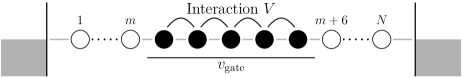
Figure 1: Schematic view of the model under consideration: A quantum dot (full circles) attached to left and right leads, each of them consisting of $m$ non-interacting sites (open circles) and a reservoir described by a continuum of states (shaded regions). The electrons on the dot (site $m+1$ to $m+5$) interact and their potential energy can be tuned by a gate voltage.

In the following we choose $t^{\prime}=0.2t$ and $t_{\rm dot}=0.5t$. The interaction strength and the potentials are constant within the quantum dot, $V_{l,l+1}=V$ and $v_{l}=v_{\rm gate}$, and zero outside. The reservoirs, chosen to be non-interacting fermions, are described by

$$\hat{H}_{L/R}=\sum_{k}\epsilon_{k}\hat{c}_{kL/R}^{+}\hat{c}_{kL/R},$$ (4)

and finally the coupling between the chain and the left reservoir reads

$$\hat{H}_{LC}=-\sum_{k}t_{k}\left(\hat{c}_{kL}^{+}\hat{c}_{1}+\hat{c}_{1}^{+}\hat{c}_{kL}\right)$$ (5)

and analogously for $\hat{H}_{CR}$. The hopping parameters $t_{k}$ are fine-tuned such that an electron at the Fermi energy is not back-scattered at the interface between the chain and the reservoirs, schmitteckert2008 $t_{k}=\sqrt{t/\pi N(\epsilon_{k})}$ where $N({\epsilon_{k}})$ is the density of states in the reservoirs. Up to this point our model is the same as the model studied by Schmitteckert and Evers [schmitteckert2008, ]. In contrast to [schmitteckert2008, ], however, we replace the discrete levels in the reservoirs by a continuum of a wide and flat band, which then leads to

$$\Gamma_{L/R} = 2\pi\sum_{k}|t_{k}|^{2}\delta(\epsilon_{F}-\epsilon_{k})$$ (6)

$$= \left.2\pi|t_{k}|^{2}N(\epsilon_{k})\right|_{k=k_{F}}=2t.$$ (7)

Notice that in the continuum limit the density of states in the reservoirs goes to infinity, and thus—in order to keep $\Gamma_{L/R}$ constant—the coupling strength between the states in the reservoirs and the chain goes to zero.

III Static density functional theory

The lattice version of DFT relies on the fact that there is a one-to-one correspondence between local potentials $\{v_{i}\}$ and the ground-state expectation values of the site occupations $\{n_{i}\}$. Therefore it is—in principle—possible to express all quantities that can be obtained from the ground-state wave function as a function of the densities. The site occupations as a function of the potentials can be found from derivatives of the ground-state energy with respect to the local potential

$$n_{i}=\frac{\partial E_{0}}{\partial v_{i}}.$$ (8)

In order to determine the potentials from the densities it is convenient to define the function

$$F(\{n_{i}\})={\rm min}_{\Psi\to\{n_{i}\}}\langle\Psi|\hat{T}+\hat{V}|\Psi\rangle,$$ (9)

where $\Psi\to\{n_{i}\}$ indicates that the minimization is constrained to such wave functions $\Psi$ that yield the given site occupations $\{n_{i}\}$. Here $\hat{T}$ and $\hat{V}$ are the kinetic and the interaction parts of the Hamiltonian, respectively. The ground-state energy is obtained by minimizing the function

$$E(\{n_{i}\})=F(\{n_{i}\})+\sum_{i}v_{i}n_{i}$$ (10)

with respect to $n_{i}$. When we minimize $E$ under the constraint of a constant particle number we obtain the potential up to an additive constant (the Lagrange multiplier):

$$v_{i}=-\frac{\partial F}{\partial n_{i}}+\lambda.$$ (11)

A major step towards the practical implementation of DFT is to employ a non-interacting auxiliary Hamiltonian $\hat{H}^{s}$ (Kohn-Sham Hamiltonian) in order to calculate the density profile,

$$\hat{H}^{s}=\hat{T}+\sum_{i}v_{i}^{s}\hat{n}_{i},$$ (12)

where the potentials $v_{i}^{s}$ have to be chosen such that in the ground-state of $H^{s}$ the site occupations $n_{i}$ are the same as in the interacting model. In analogy to the interacting system, the ground-state energy of the Kohn-Sham system is found by minimizing

$$E^{s}(\{n_{i}\})=F^{s}(\{n_{i}\})+\sum_{i}v_{i}^{s}n_{i}.$$ (13)

Combining (10) and (13) yields

$$E(\{n_{i}\})=E^{s}(\{n_{i}\})+E^{\rm HXC}(\{n_{i}\})+\sum_{i}(v_{i}-v_{i}^{s})n_{i},$$ (14)

with the Hartree-exchange-correlation energy defined by

$$E^{\rm HXC}(\{n_{i}\})=F(\{n_{i}\})-F^{s}(\{n_{i}\}).$$ (15)

The condition that both $E$ and $E^{s}$ are minimal for the same set of site occupations $n_{i}$ requires that

$$v_{i}^{s}=v_{i}+\frac{\partial E^{\rm HXC}}{\partial n_{i}}.$$ (16)

Up to this point no approximations have been employed. However to determine $E^{\rm HXC}$ at a given density exactly is as demanding as finding the ground state energy for a given potential. The hope is that there exist good approximations for $E^{\rm HXC}$ that are accessible with low numerical cost but still allow good estimates for the ground-state energy and density. Here and in the following we will compare three different approximations: the local-density approximation, the optimized effective potential (so-called exact exchange) approximation, and finally a method based on the exact diagonalization of small clusters.

III.1 Local density approximation

In the LDA one writes $E^{\rm HXC}$ as the sum of the (non-local) Hartree energy plus an exchange-correlation energy which depends only on the local density,

$$E^{\rm HXC}_{\rm LDA}(\{n_{i}\})=V\sum_{i}n_{i}n_{i+1}+\sum_{i}\epsilon_{\rm XC}(n_{i}).$$ (17)

The local exchange-correlation energy $\epsilon_{\rm XC}(n)$ is determined from the ground-state energy density of a homogeneous system at the same density. For the one-dimensional lattice models this quantity can be calculated using the Bethe ansatz, see Refs. [lima2003, ; schenk2008, ]. Notice that in the Hamiltonian we study the interaction strength depends on position, and an ambiguity arises how to determine the exchange-correlation potential for those sites which interact only with one neighbor. For simplicity we used in our numerical implementation of the LDA the same function $\epsilon^{\rm xc}(n)$ for all interacting lattice sites, i.e., number $m+1$ to $m+5$.

III.2 Optimized effective potential

In the OEP approach the Hartree-exchange-correlation energy is

$$E^{\rm HXC}_{\rm OEP}(\{n_{i}\})=V\sum_{i}n_{i}n_{i+1}+E^{\rm X}(\{n_{i}\})$$ (18)

with the Fock-like exchange energy

$$E^{\rm X}=-V\sum_{i}\langle\hat{c}^{+}_{i}\hat{c}_{i+1}\rangle\langle\hat{c}^{+}_{i+1}\hat{c}_{i}\rangle.$$ (19)

We calculate the ground state expectation values $\langle\hat{c}^{+}_{i}\hat{c}_{i+1}\rangle$ etc. for a non-interacting system coupled to reservoirs using the Green’s function technique, see section IV. The Kohn-Sham equations (16) are most conveniently solved by iteration. Starting with an initial guess for the potentials $v_{i}^{s}$ we calculate the corresponding site occupations $n_{i}$ and the Hartree-exchange-correlation energy $E^{\rm HXC}$. Since in the OEP approach $E^{\rm HXC}$ depends only implicitly on $n_{i}$ we rewrite Eq. (16) using

$$\frac{\partial E^{\rm HXC}}{\partial n_{i}}=\sum_{j}\frac{\partial E^{\rm HXC}}{\partial v_{j}^{s}}\frac{\partial v_{j}^{s}}{\partial n_{i}}$$ (20)

where the derivatives of $E^{\rm HXC}$ with respect to the $v_{j}^{s}$ are calculated numerically and $\partial v_{j}^{s}/\partial n_{i}$ is obtained by matrix inversion from $\partial n_{i}/\partial v_{j}^{s}$. Finally we obtain a new set of Kohn-Sham potentials $v_{i}^{s}$. The whole procedure is repeated until convergence, i.e., until the difference between old and new potentials is smaller than some given cutoff.

The fact that we use a continuum of states to describe the reservoirs simplifies the task to solve Eq. (16) considerably: Since the states in the reservoirs are only infinitesimally weakly coupled to the dot, the Hartree-exchange-correlation potential in the reservoirs disappears, so that the number of potentials $v_{i}^{s}$ to be determined self-consistently equals the chain length $N$.

III.3 Exact diagonalization

In our model Hamiltonian electrons interact only in a spatially confined region. In the non-interacting regions we find numerically (e.g., within the OEP approach, see Fig. 6 below; compare also Ref. [schmitteckert2008, ] for density matrix renormalization group (DMRG) results) only small exchange-correlation potentials. This finding motivated us to use the exchange-correlation energy of a small cluster consisting of the interacting region plus a small number of non-interacting sites as an approximation for the exchange-correlation energy of the system attached to reservoirs:

$$E^{\rm HXC}_{\rm ED}(\{n_{i}\})=F_{\rm ED}(\{n_{i}\})-F_{\rm ED}^{s}(\{n_{i}\})$$ (21)

where $F_{\rm ED}(\{n_{i}\})$ and $F_{\rm ED}^{s}(\{n_{i}\})$ are exact on the small cluster and can be obtained by numerical diagonalization.

In this approach we have to fine-tune the local potentials of three different Hamiltonians such that all the three yield the same local densities: (i) a cluster of interacting electrons with potentials $u_{i}$, (ii) a cluster of non-interacting electrons with potentials $u_{i}^{s}$, and (iii) the Kohn-Sham Hamiltonian of the extended quantum dot attached to reservoirs with $v_{i}^{s}=v_{i}+v_{i}^{\rm HXC}$ where $v_{i}^{\rm HXC}=u_{i}-u_{i}^{s}$ on the cluster sites and zero outside. Again, in a practical scheme the fine-tuning procedure is performed by iteration. The task to determine the potentials $u_{i}$ that correspond to a given set of site occupations $n_{i}$ is nontrivial for an interacting system and limits the cluster size in our approach to approximately 12 to 14 sites.

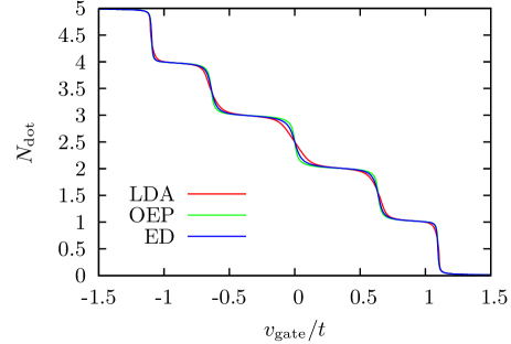
Figure 2: Particle number on the dot, $N_{\rm dot}$, as function of the gate voltage, $v_{\rm gate}$, for $V/t=0.25$ obtained within density functional theory with three different approximations for the exchange-correlation energy: the local-density approximation (LDA), optimized effective potential (OEP) and a method based on the exact diagonalization of short chains (ED). Here the chains have a length of nine lattice sites.

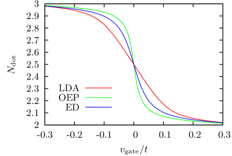
Figure 3: $N_{\rm dot}$ as function of $v_{\rm gate}$ around to the central step for $V/t=0.25$; for this interaction strength OEP is still close to the exact result.

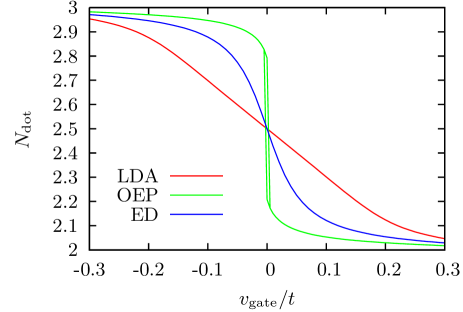
Figure 4: $N_{\rm dot}$ as function of $v_{\rm gate}$ for $V/t=0.5$. Solving the OEP equations iteratively as a function of gate voltage two solutions are found close to $v_{\rm gate}=0$.

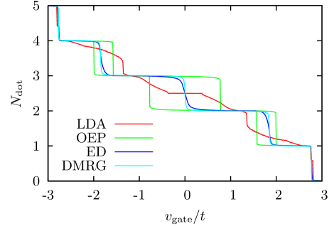
Figure 5: $N_{\rm dot}$ as function of $v_{\rm gate}$ for $V/t=2$. For comparison we also include the DMRG results of [schmitteckert2008, ].

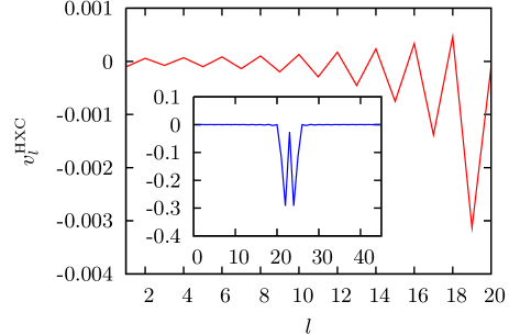
Figure 6: Hartree-exchange-correlation potential $v^{\rm HXC}_{l}$ in OEP for a long chain with $m=20$ non-interacting sites attached on each side of the five-site quantum dot with parameters $v_{\rm gate}/t=0.5$ and $V/t=0.5$. In the figure, $v^{\rm HXC}_{l}$ is shown for the non-interacting sites $l=1,\ldots,m$ and for the whole chain in the inset.

III.4 Results

In the following we focus on the particle number in the interacting region, $N_{\rm dot}$, as function of the gate voltage, $V_{\rm gate}$, comparing results for the three aforementioned approaches LDA, OEP, and ED, respectively. The data are obtained for a chain of nine sites, i.e., the five-site quantum dot plus two non-interacting sites on each side of it. Fig. 2 shows $N_{\rm dot}$ for weak interaction strength, $V/t=0.25$. The three curves nearly coincide with exception of the regions close to the steps, in particular around $V_{\rm gate}=0$. Here, as pointed out in Fig. 3, the step appears steeper in OEP and flatter in LDA compared to ED.

This trend continues at stronger interaction, $V/t=0.5$, where in OEP the particle number even jumps close to $V_{\rm gate}=0$ with a small hysteresis region of two stable solutions, while the LDA step flattens out even more, as displayed in Fig. 4.

In the strong coupling regime (Fig. 5) where $V/t=2$, comparison with the exact densities obtained from DMRG calculations schmitteckert2008 shows that LDA and OEP fail completely, while the ED results agree reasonably well with the exact data. Note however that the DMRG data are for a five-site quantum dot with two non-interacting sites attached on the right and three on the left, and that the reservoirs are described by a finite set of the order of 100 discrete levels instead of a continuum. From the above observations we conclude that in DFT calculations for lattice models LDA and OEP results are reliable in the weak interaction regime. In particular, it can be shown that the OEP density profile is exact to linear order in the interaction strength $V$. On the other hand, for strongly correlated systems more sophisticated methods like the ED cluster approach are required, even for static properties.

As already mentioned in Sec. III.C, far from the interacting region the potential $v_{l}^{\rm HXC}$ becomes very small. This is explicitly demonstrated in Fig. 6: In the leads the Hartree-exchange-correlation potential, $v_{l}^{\rm HXC}$, within OEP, is found to be about three orders of magnitude smaller than in the interacting region (see inset).

IV Transport

DFT as presented in the previous sections is a ground state theory. However generalizations are available which allow to calculate densities at finite temperature and under non-equilibrium conditions runge1984 and thus—via the continuity equation—the current through the quantum dot. The goal of this section is to calculate the DC-conductance of the quantum dot when a small voltage difference is applied. We will extract the DC-conductance from a calculation of the dynamic density response function, and the connection to the standard Meir-Wingreen formula meir92 will be made.

IV.1 Conductance from density response

We start with the current flowing from the left reservoir into the dot, which is given by the time derivative of the particle number in the reservoir,

$$I=e\dot{N}_{L}=e\sum_{k}\dot{n}_{kL},$$ (22)

i.e., $I(\omega)=-ie\omega N_{L}(\omega)$, where $-e$ is the electron charge. The frequency dependent variation in the particle number $N_{L}(\omega)$ appears as a response to a perturbation in the (single particle) Hamiltonian of the form

$$\delta\hat{H}^{s}=\sum_{\alpha}\hat{n}_{\alpha}\delta v_{\alpha}^{s},$$ (23)

where $\delta v_{\alpha}^{s}=\delta v_{\alpha}^{\rm ext}+\delta v_{\alpha}^{\rm HXC}$ is the sum of an external potential and the induced Hartree-exchange-correlation potential. The summation $\alpha$ includes both reservoir, $\alpha=kL,kR$ and chain degrees of freedom, $\alpha=l$. The variation of the density at site $\beta$ is then

$$\delta n_{\beta}(\omega)=-i\sum_{\alpha}\int\frac{d\epsilon}{2\pi}{\cal G}_{\epsilon+\omega}(\beta,\alpha)\delta v_{\alpha}^{s}(\omega){\cal G}_{\epsilon}(\alpha,\beta),$$ (24)

where $\cal G_{\epsilon}(\alpha,\beta)$ is the (zero temperature) Green’s function of the single-particle Hamiltonian. It is useful to distinguish the Green’s function of the reservoirs from the Green’s function of the chain, and in the following we will use the symbols $g_{\epsilon}(kL)$ for the (left) reservoir Green’s function and $G_{\epsilon}(l,l^{\prime})$ for a chain Green’s function. The latter is given by

$$G_{\epsilon}(l,l^{\prime})=G^{0}_{\epsilon}(l,l^{\prime})+\sum_{m}G^{0}_{\epsilon}(l,m)\Sigma_{\epsilon}(m)G_{\epsilon}(m,l^{\prime}),$$ (25)

were $G^{0}_{\epsilon}(l,l^{\prime})$ is the bare Green’s function, i.e., the one for $t_{k}=0$, and the self-energy $\Sigma_{\epsilon}(m)$ appears due to the coupling to the reservoirs. For our model Hamiltonian $\Sigma_{\epsilon}(m)$ is non-zero only on the first and last site of the chain, $m=1,N$. The explicit expression for the first site is

$$\Sigma_{\epsilon}(1)=\sum_{k}|t_{k}|^{2}g^{0}_{\epsilon}(kL),$$ (26)

where

$$g^{0}_{\epsilon}(kL)=\frac{1}{\epsilon-\epsilon_{k}+i\delta\,{\rm sgn}(\epsilon-\mu)},\quad\delta=0^{+}$$ (27)

is the bare Green’s function of state $k$ in the left lead. For energies close to the chemical potential and for our special choice of the couplings $t_{k}$ the self-energy then assumes the value $\Sigma_{\epsilon}(1)=-it\,{\rm sgn}(\epsilon-\mu)$. The Green’s function for the states in the left reservoir finally is

$$g_{\epsilon}(kL)=g^{0}_{\epsilon}(kL)+g^{0}_{\epsilon}(kL)\,t_{k}\,G_{\epsilon}(1,1)\,t_{k}\,g^{0}_{\epsilon}(kL).$$ (28)

The variation of the particle number in the reservoirs can be represented graphically as

(29)

where the full line denotes a reservoir Green’s function, $g^{0}_{\epsilon}(kL)$ or $g^{0}_{\epsilon}(kR)$, the broken line is the chain Green’s function $G_{\epsilon}(l,l^{\prime})$ and the cross corresponds to a hopping process between reservoir and chain. In order to calculate the DC conductance of the system we have to evaluate these diagrams for small but finite frequency, and we have to identify contributions that diverge as $1/\omega$ as $\omega$ goes to zero. Such divergences are found in diagrams c), d) and e). In all three cases the diverging contribution arises from the region in the $\epsilon$-integration where $\epsilon<\mu<\epsilon+\omega$. For diagram c), for instance, the relevant contribution is

$$\delta N_{L}^{c)} = -i\int_{\mu-\omega}^{\mu}\frac{d\epsilon}{2\pi}G_{\epsilon+\omega}(1,1)$$

$$\times\sum_{k}t_{k}^{2}\left(\frac{1}{\epsilon+\omega-\epsilon_{k}+i\delta}\right)^{2}\frac{1}{\epsilon-\epsilon_{k}-i\delta}\delta v_{kL}^{s}.$$

In the next step the $k$-summation in the second line is replaced by an integral. Clearly the dominant contribution to the $k$-integration comes from a small region around the Fermi energy. Assuming that neither the potential $\delta v_{kL}^{s}$ nor the coupling $t_{k}$ are singular around the Fermi momentum we find $\sum_{k}(\dots)=i\Gamma_{L}\delta v^{s}_{kL}/\omega^{2}$, where the potential has to be evaluated at the Fermi energy. The variation of the particle number in the left reservoir hence is

$$\delta N_{L}^{c)}=\frac{\delta v^{s}_{kL}}{2\pi\omega}\Gamma_{L}G^{R}_{\mu}(1,1).$$ (31)

The retarded chain Green’s function at the chemical potential, $G^{R}_{\mu}(1,1)$, appears since $\epsilon+\omega>\mu$ in Eq. (IV.1) and we consider the limit $\omega\to 0$.

Using similar arguments for the diagrams d) and e), we find

$$\delta N_{L}^{d)} = -\frac{\delta v_{kL}^{s}}{2\pi\omega}\Gamma_{L}G^{A}_{\mu}(1,1)$$ (32)

$$\delta N_{L}^{e)} = \frac{i\delta v_{kL}^{s}}{2\pi\omega}\left[\Gamma_{L}G^{R}_{\mu}(1,1)\Gamma_{L}G^{A}_{\mu}(1,1)\right]$$ (33)

$$+\frac{i\delta v_{kR}^{s}}{2\pi\omega}\left[\Gamma_{L}G^{R}_{\mu}(1,N)\Gamma_{R}G^{A}_{\mu}(N,1)\right].$$

Using finally the relation

$$G^{R}_{\mu}(1,1)-G^{A}_{\mu}(1,1) = -iG^{R}_{\mu}(1,1)\Gamma_{L}G^{A}_{\mu}(1,1)$$ (34)

$$-iG^{R}_{\mu}(1,N)\Gamma_{R}G^{A}_{\mu}(N,1)$$

the complete singular contribution to the density in the reservoir reads

$$\delta N_{L}=(\delta v_{kR}^{s}-\delta v_{kL}^{s})\frac{i}{2\pi\omega}\Gamma_{L}G^{R}_{\mu}(1,N)\Gamma_{R}G^{A}_{\mu}(N,1).$$ (35)

This enables us to write the current as the product of a conductance $G$ and a voltage $U^{\rm tot}$,

$$I=-ie\omega\delta N_{L}=GU^{\rm tot},$$ (36)

where the expression for the conductance agrees with the standard Meir-Wingreen formula for non-interacting electrons,

$$G=\frac{e^{2}}{2\pi\hbar}\Gamma_{L}G^{R}_{\mu}(1,L)\Gamma_{R}G^{A}_{\mu}(L,1),$$ (37)

and the voltage is the sum of an externally applied voltage and an exchange-correlation contribution, $U^{\rm tot}=U^{\rm ext}+U^{\rm xc}$, with

$$eU^{\rm ext}=\delta v^{\rm ext}_{kR}-\delta v^{\rm ext}_{kL},\quad eU^{\rm xc}=\delta v^{\rm HXC}_{kR}-\delta v^{\rm HXC}_{kL}.$$ (38)

Notice that only the exchange-correlation potentials in the reservoirs but not in the chain contribute to the total voltage. Our result is thus consistent with [stefanucci2004, ] where it has been shown that the exact current can be expressed in terms of a Landauer-type formula landauer1957 in which the electro-chemical potential of the leads is shifted by the voltage-induced variation of the exchange correlation potential, and with the statements of Refs. [mera2010, ; koentopp2006, ] that static DFT gives the exact linear-response conductance provided that the dynamic exchange-correlation potential vanishes deep inside the leads.

Notice that $U^{\rm xc}$ is a purely dynamic effect that cannot be captured by any adiabatic approximation. However, $U^{\rm xc}$ can be assessed via reverse engineering: If we know the exact static densities and the exact conductance, then the ratio of the exact conductance and the DFT conductance, Eq. (37), is equal to the ratio of the total and the external voltage, $G^{\rm exact}/G=U^{\rm tot}/U^{\rm ext}$.

IV.2 Results

Figure 7 shows the conductance as a function of the gate voltage in the case of a weak interaction $V=0.25t$. One observes five resonances at the gate voltages where the particle number on the dot changes, compare Fig. 2. LDA overestimates the width of the resonances just as it overestimates the width of the steps in the particle number. We also include OEP and Hartree-Fock (HF) results in the figure. For weak interaction both methods predict identical charge densities, for the present interaction strength the difference in particle number on the dot is for the two methods less than $7\cdot 10^{-3}$. Also the conductances are close to each other.

In Fig. 8 we show the region close to zero gate voltage in more detail. Near the resonance HF and OEP are almost indistinguishable, however far from the resonance a significantly different conductance is found. This difference is due to the exchange-correlation contribution to the voltage, $U^{\rm xc}$. To substantiate this point we analyze the correction to the conductance to first order in the interaction strength $V$. In this case HF yields the exact conductance.

However, as demonstrated in Fig. 9 the conductances obtained by OEP and HF differ—although the densities are identical. Figure 9 has been obtained for a chain length $N=9$, but we have checked that even for much longer chains (up to $N=25$) there is no visible change in the results. This means that $U^{\rm xc}$ remains nonzero even far from the interacting region.

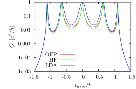
Figure 7: Conductance $G$ as function of $v_{\rm gate}$ for $V/t=0.25$. The OEP and LDA curves are obtained within static density functional theory as explained in the text. “HF” corresponds to a self-consistent Hartree-Fock calculation.

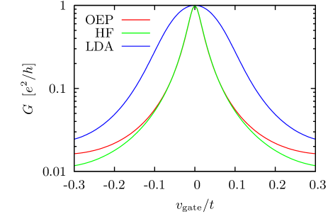
Figure 8: Conductance $G$ as function of $v_{\rm gate}$ close to the central peak for $V/t=0.25$.

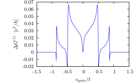
Figure 9: Linear contribution $G^{(1)}$ of the expansion of the conductance $G=G^{(0)}+G^{(1)}V/t+G^{(2)}(V/t)^{2}+\ldots$ in powers of the interaction strength. The difference between the OEP result and the exact HF conductance, $\Delta G^{(1)}=G^{(1)}_{\rm OEP}-G^{(1)}_{\rm HF}$, is plotted as function of $v_{\rm gate}$.

Figure 10 shows the conductance for the relatively strong interaction strength $V=2t$, comparing LDA, ED and the numerically exact conductance obtained with the DMRG in Ref. [schmitteckert2008, ]. Although the position of the resonances is not bad in LDA the method predicts conductances that differ several orders of magnitude from the exact results. The ED results are considerably better. Near the resonances ED predicts conductances that are close to the DMRG values.

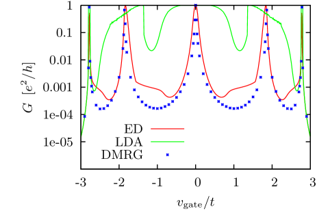
Figure 10: Conductance $G$ as function of $v_{\rm gate}$ for $V/t=2$; the DMRG data are taken from Ref.  [schmitteckert2008, ].

V Summary and Conclusions

We studied the ground state density profile and the conductance of a model quantum dot comparing DFT and exact results. The electron density in the ground state can be obtained reliably using non-local exchange-correlation potentials. While for weak interaction the OEP approach gives good results, in the case of intermediate or strong interaction strengths a non-local potential extracted from the exact diagonalization of small clusters (DFT+ED) works well.

For the conductance our results are not so clear-cut. In our simple model we find five well separated resonances as a function of the gate voltage. Static DFT reproduces very well the position and the width of these resonances. However, in contrast to model cases where the Friedel sum rule allows to express the conductance in terms of the equilibrium charge density, compare Ref. [mera2010, ], in our model system such a sum rule is not valid. As a consequence the DFT conductance is not exact, and we find pronounced deviations in the conductance valleys between the resonances.

As the origin of these discrepancies we have identified a dynamical exchange-correlation correction to the applied voltage, which is non-zero even when the reservoirs are far from the interacting region. We believe that this finding is related to “ultra-non-locality” which is an inherent problem in time-dependent density functional theory vignale1996 ; sai2005 .

We thank C. Schuster for fruitful discussions as well as the Deutsche Forschungsgemeinschaft (TRR80) for financial support.

References

- (1) P. Hohenberg and W. Kohn, Phys. Rev. 136, B864 (1964).
- (2) W. Kohn and L. J. Sham, Phys. Rev. 140, A1133 (1965).
- (3) O. Gunnarsson and K. Schönhammer, Phys. Rev. Lett. 56, 1968 (1986).
- (4) K. Schönhammer and O. Gunnarsson, J. Phys. C 20, 3675 (1987).
- (5) K. Schönhammer, O. Gunnarsson, and R. M. Noack, Phys. Rev. B 52, 2504 (1995).
- (6) N. A. Lima, M. F. Silva, L. N. Oliveira, and K. Capelle, Phys. Rev. Lett. 90, 146402 (2003).
- (7) U. Schwingenschlögl and C. Schuster, Ann. Phys. (Berlin) 520, 525 (2008).
- (8) S. Schenk, M. Dzierzawa, P. Schwab, and U. Eckern, Phys. Rev. B 78, 165102 (2008).
- (9) M. Dzierzawa, U. Eckern, S. Schenk, and P. Schwab, Phys. Status Solidi B 246, 941 (2009).
- (10) M. Brandbyge, J.-L. Mozos, P. Ordejon, J. Taylor, and K. Stokbro, Phys. Rev. B 65, 165401 (2002).
- (11) A. R. Rocha, V. M. Garcia-Suarez, S. Bailey, C. Lambert, J. Ferrer, and S. Sanvito, Phys. Rev. B 73, 085414 (2006).
- (12) M. Koentopp, C. Chang, K. Burke, and R. Car, J. Phys.: Condens. Matter 20, 083203 (2008).
- (13) P. Schmitteckert and F. Evers, Phys. Rev. Lett. 100, 086401 (2008).
- (14) H. Mera, K. Kaasbjerg, Y. M. Niquet, and G. Stefanucci, Phys. Rev. B 81, 035110 (2010).
- (15) E. Runge and E. K. U. Gross, Phys. Rev. Lett. 52, 997 (1984).
- (16) Y. Meir and N. S. Wingreen, Phys. Rev. Lett. 68, 2512 (1992).
- (17) G. Stefanucci and C.-O. Almbladh, Europhysics Lett. 67, 14 (2004).
- (18) R. Landauer, IBM J. Res. Develop. 1, 223 (1957).
- (19) M. Koentopp, K. Burke, and F. Evers, Phys. Rev. B 73, 121403(R) (2006).
- (20) G. Vignale and W. Kohn, Phys. Rev. Lett. 77, 2037 (1996).
- (21) N. Sai, M. Zwolak, G. Vignale, and M. Di Ventra, Phys. Rev. Lett. 94, 186810 (2005).