Non-symmetrized hyperspherical harmonic basis for $A$–bodies

Abstract

The use of the hyperspherical harmonic (HH) basis in the description of bound states in an $A$-body system composed by identical particles is normally preceded by a symmetrization procedure in which the statistic of the system is taken into account. This preliminary step is not strictly necessary; the direct use of the HH basis is possible, even if the basis has not a well defined behavior under particle permutations. In fact, after the diagonalization of the Hamiltonian matrix, the eigenvectors reflect the symmetries present in it. They have well defined symmetry under particle permutation and the identification of the physical states is possible, as it will be shown in specific cases. The problem related to the large degeneration of the basis is circumvented by constructing the Hamiltonian matrix as a sum of products of sparse matrices. This particular representation of the Hamiltonian is well suited for a numerical iterative diagonalization, where only the action of the matrix on a vector is needed. As an example we compute bound states for systems with $A=3-6$ particles interacting through a short-range central interaction. We also consider the case in which the potential is restricted to act in relative $s$-waves with and without the inclusion of the Coulomb potential. This very simple model predicts results in qualitative good agreement with the experimental data and it represents a first step in a project dedicated to the use of the HH basis to describe bound and low energy scattering states in light nuclei.

I Introduction

The ab initio description of light nuclear systems, starting from the nucleon-nucleon (NN) interaction, requires well established methods to solve the Schrödinger equation. Among them, the Green function Monte Carlo (GFMC) method has been extensively used to describe light nuclei up to $A=10$ and the no-core shell model (NCSM) up to $A=12$ gfmc ; ncsm . In the $A\leq 4$ systems, well established methods for treating both bound and scattering states exist as the Faddeev equations ($A=3$) and the Faddeev-Yakubovsky equations ($A=4$) in configuration or momentum space, and the Hyperspherical Harmonic (HH) expansion. All these methods have proven to be of great accuracy and they have been tested using different benchmarks benchmark1 ; benchmark2 ; benchmark3 .

The HH method provides a systematic way of constructing a complete basis for the expansion of the $A$-particle wave function and its use in the $A>4$ systems has been subject of intense investigations over the last years. In the specific case of application to nuclear physics, the wave function has to be antisymmetric and, therefore, the HH basis has been managed to produce basis states having well defined properties under particle permutations. Different schemes to construct hyperspherical functions with an arbitrary permutational symmetry are given in Refs. novo94 ; barnea95 ; barnea99 . Recently, a procedure for constructing HH functions in terms of a single particle basis has been proposed in Ref. timofeyuk:08 .

In a different approach, the authors have used the HH basis, without a previous symmetrization procedure, to describe bound states in three- and four-particle systems mario . It has been observed that the eigenvectors of the Hamiltonian matrix reflects the symmetries present in it, even if it has been constructed using the non-symmetrized basis. The only requirement was to include all the HH basis elements having the same grand angular quantum number $K$. It is a property of the HH basis that basis elements having well defined behavior under particle permutation can be constructed as a linear combination of HH elements having the same value of $K$. Therefore, if the Hamiltonian commutes with the group of permutations of $A$ objects, $S_{A}$, the diagonalization procedure generates eigenvectors having well defined permutation symmetry that can be organized in accordance with the irreducible representations of $S_{A}$. Moreover, identifying those eigenvectors with the desired symmetry, the corresponding energies can be considered variational estimates. In particular, in Ref. mario , it was possible to identify a subset of eigenvectors and eigenvalues corresponding exactly to those that would be obtained performing the preliminary symmetrization of the states. It should be noticed that the simplicity of using the HH basis without a preliminary antisymmetrization step, has to be counterbalanced with the large dimension of the matrices to be diagonalized. However, at present, different techniques are available to treat (at least partially) this problem.

In the present article we continue the study of the non-symmetrized HH basis, extending the applications to systems with $A>4$. In pursuit of this goal, we have developed a particular representation of the Hamiltonian matrix, which is systematic with respect to the number of particles and well suited for a numerical implementation. As mentioned, one of the main problem in using the HH basis is its large degeneracy, resulting in very large matrices. On the other hand, the potential energy matrix, expressed as a sum of pairwise interactions, cannot connect arbitrary basis elements differing in some specific quantum numbers. This means that in some representation each pairwise-interaction term has to be represented by a sparse matrix. For example, the matrix representation of the potential $V(1,2)$, constructed in terms of basis elements in which the quantum numbers of particles $(1,2)$ are well defined, is sparse in $A\geq 3$ systems. In fact, its matrix elements connecting basis elements with different quantum numbers labelling states which do not involve particles $(1,2)$ are zero. A problem arises when the matrix elements of the generic term $V(i,j)$, defining the interaction between particles $(i,j)$, has to be calculated using basis elements in which the quantum numbers of particles $(i,j)$ are not well defined. One operative way to solve this problem consists in rotating the basis to a system of coordinates in which particles $(i,j)$ have well defined quantum numbers. This makes the matrix $V(i,j)$ sparse. However, we would like the rotation matrix to be sparse too, which in general it is not true. This last problem is solved noticing that the rotation matrix can be expressed as a product of sparse matrices, each one representing a rotation which involves a permutation of particles of successive numbering. After these manipulations the potential energy matrix results in a sum of products of sparse matrices suitable for numerical implementations.

An advantage in using the non-symmetrized HH basis appears when symmetry breaking terms are present in the Hamiltonian. In the case of the nuclear Hamiltonian with charge-symmetry breaking terms, this means that different total isospin components $T$ are present in the wave function. For example, the three-nucleon bound state wave function includes $T=1/2,3/2$ components and the four-nucleon bound state wave function includes $T=0,1,2$ components, requiring the inclusion of different spatial symmetries in the wave function. Therefore, considering all the possible spin and isospin components, the number of HH states having well defined spatial symmetries, necessary to construct the wave function, and the dimension of the non-symmetrized basis is comparable. High isospin components are in general a small part of the total wave function. They are difficult to include in the antisymmetrized basis since appreciably increases the number of basis elements and, at the same time, they improve very little the description of the state. In practical cases they are disregarded, or partially included, with the consequence that the occupation probabilities of the high isospin states are not always well determined (see Ref. viviani05 ). Conversely, using the non-symmetrized basis, all the isospin components are automatically generated. As an example we will show results for $A=3-6$ systems using short-range central interactions with and without the inclusion of the Coulomb potential.

To summarize, in this paper we present the implementation of the non-symmetrized HH basis for $A$-body system using the factorization of the potential energy matrix mentioned before. In order to give a detailed description of this construction, we consider only spatial degrees of freedom; accordingly, we show examples using a central interaction. The diagonalization of the Hamiltonian produces eigenvectors organized in multiplets of the dimension of the corresponding irreducible representation of $S_{A}$, and the different symmetries will be identified using the appropriate Casimir operator. Not all the states belonging to a particular representation can be antisymmetrized using the spin-isospin functions of $A$ nucleons and, therefore, these states are not physical. It should be noticed that the physical states could appear in very high positions of the spectrum, in particular this is the case for $A>4$ systems. On the other hand, the iterative methods, as the Lanczos method, used to search selected eigenvalues and eigenvectors of large matrices are more efficient for the extreme ones. To this respect, we have found very convenient to use the symmetry-adapted Lanczos method proposed in Ref. slanczos , which restricts the search to those states having a particular symmetry. When possible, comparisons to different results in the literature will be done. Since we have in mind the description of light nuclear systems using realistic interactions, this study can be considered a preliminary step in the use of this technique.

The paper is organized as follows; section II is devoted to a brief description of the HH basis. In sections III the expression for the potential energy matrix in terms of HH states is given. In section IV the results for the models proposed are shown. Section V includes a brief discussion of the results and the perspectives of the present work.

II The Harmonic Hyperspherical basis for $A$ bodies

In this section we introduce the notation and we present a brief overview of the properties of the HH basis.

II.1 Basic properties of the HH basis

In accord with Ref.mario , we start with the following definition of the Jacobi coordinates for an $A$ body system with Cartesian coordinates $\mathbf{r}_{1}\dots\mathbf{r}_{A}$

$$\mathbf{x}_{N-j+1}=\sqrt{\frac{2m_{j+1}M_{j}}{(m_{j+1}+M_{j})m}}\,(\mathbf{r}_{j+1}-\mathbf{X}_{j})\,,\qquad j=1,\dots,N\,,$$ (1)

where $m$ is a reference mass, $N=A-1$, and where we have defined

$$M_{j}=\sum_{i=1}^{j}m_{i}\,,\qquad\mathbf{X}_{j}=\frac{1}{M_{j}}\sum_{i=1}^{j}m_{i}\mathbf{r}_{i}\,.$$ (2)

Let us note that if all the masses are equal, $m_{i}=m\,$, Eq. (1) simplifies to

$$\mathbf{x}_{N-j+1}=\sqrt{\frac{2j}{j+1}}\,(\mathbf{r}_{j+1}-\mathbf{X}_{j})\,,\qquad j=1,\dots,N\,.$$ (3)

For a given set of Jacobi coordinates $\mathbf{x}_{1},\dots,\mathbf{x}_{N}$, we can introduce the hyperradius $\rho$

$$\rho=\bigg{(}\sum_{i=1}^{N}x_{i}^{2}\bigg{)}^{1/2}=\bigg{(}2\sum_{i=1}^{A}(\mathbf{r}_{i}-\mathbf{X})^{2}\bigg{)}^{1/2}=\bigg{(}\frac{2}{A}\sum_{j>i}^{A}(\mathbf{r}_{j}-\mathbf{r}_{i})^{2}\bigg{)}^{1/2}\,,$$ (4)

and the hyperangular coordinates $\Omega_{N}$

$$\Omega_{N}=(\hat{x}_{1},\dots,\hat{x}_{N},\phi_{2},\dots,\phi_{N})\,,$$ (5)

with the hyperangles $\phi_{i}$ defined via

$$\cos\phi_{i}=\frac{x_{i}}{\sqrt{x_{1}^{2}+\dots+x_{i}^{2}}}\,,\qquad i=2,\dots,N\,.$$ (6)

The radial components of the Jacobi coordinates can be expressed in terms of the hyperspherical coordinates

$$x_{N}=\rho\cos\phi_{N}$$ (7)

$$x_{N-1}=\rho\sin\phi_{N}\cos\phi_{N-1}$$

$$\qquad\vdots$$

$$x_{i}=\rho\sin\phi_{N}\cdots\sin\phi_{i+1}\cos\phi_{i}$$

$$\qquad\vdots$$

$$x_{2}=\rho\sin\phi_{N}\cdots\sin\phi_{3}\cos\phi_{2}$$

$$x_{1}=\rho\sin\phi_{N}\cdots\sin\phi_{3}\sin\phi_{2}\,.$$

Using the above hyperspherical angles $\Omega_{N}$, the surface element becomes

$$d\Omega_{N}=\sin\theta_{1}\,d\theta_{1}\,d\varphi_{1}\prod_{j=2}^{N}\sin\theta_{j}\,d\theta_{j}\,d\varphi_{j}(\cos\phi_{j})^{2}(\sin\phi_{j})^{3j-4}d\phi_{j}\,,$$ (8)

and the Laplacian operator

$$\Delta=\sum_{i=1}^{N}\nabla_{\mathbf{x}_{i}}^{2}=\left(\frac{\partial^{2}}{\partial\rho^{2}}+\frac{3N-1}{\rho}\frac{\partial}{\partial\rho}+\frac{\Lambda_{N}^{2}(\Omega_{N})}{\rho^{2}}\right)\,,$$ (9)

where the $\Lambda_{N}^{2}(\Omega_{N})$ is the generalization of the angular momentum and is called grand angular operator.

The HH functions ${\mathcal{Y}}_{[K]}(\Omega_{N})$ are the eigenvectors of the grand angular momentum operator

$$\bigg{(}\Lambda_{N}^{2}(\Omega_{N})+K(K+3N-2)\bigg{)}{\mathcal{Y}}_{[K]}(\Omega_{N})=0\,.$$ (10)

They can be expressed in terms of the usual harmonic functions $Y_{lm}(\hat{x})$ and of the Jacobi polynomials $P_{n}^{a,b}(z)$. In fact, the explicit expression for the HH functions is

$${\mathcal{Y}}_{[K]}(\Omega_{N})=\left[\prod_{j=1}^{N}Y_{l_{j}m_{j}}(\hat{x}_{j})\right]\left[\prod_{j=2}^{N}\,{}^{(j)}\!{\mathcal{P}}_{K_{j}}^{\alpha_{l_{j}},\alpha_{K_{j-1}}}(\phi_{j})\right]\,,$$ (11)

where $[K]$ stands for the set of quantum numbers $l_{1},\dots,l_{N},m_{1},\dots,m_{N},n_{2},\dots,n_{N}$, and the hyperspherical polynomial is

$${}^{(j)}{\mathcal{P}}_{K_{j}}^{\alpha_{l_{j}},\alpha_{K_{j-1}}}(\phi_{j})={\mathcal{N}}_{n_{j}}^{\alpha_{l_{j}},\alpha_{K_{j}}}(\cos\phi_{j})^{l_{j}}(\sin\phi_{j})^{K_{j-1}}P^{\alpha_{K_{j-1}},\alpha_{l_{j}}}_{n_{j}}(\cos 2\phi_{j})\,,$$ (12)

with the $K_{j}$ quantum numbers defined as

$$K_{j}=\sum_{i=1}^{j}(l_{i}+2n_{i})\,,\qquad n_{1}=0\,,\qquad K\equiv K_{N}\,.$$ (13)

The normalization factor is

$${\cal N}_{n}^{\alpha\beta}=\sqrt{\frac{2(2n+\alpha+\beta+1)n!\,\Gamma(n+\alpha+\beta+1)}{\Gamma(n+\alpha+1)\Gamma(n+\beta+1)}}\,,$$ (14)

where, for the special choice of hyperangles given by Eq. (7), $\alpha_{K_{j}}=K_{j}+3j/2-1$ and $\alpha_{l_{j}}=l_{j}+1/2$. The quantum number $K\equiv K_{N}$ is also known as the grand angular momentum.

The HH functions are normalized

$$\int d\Omega_{N}\bigg{(}{\mathcal{Y}}_{[K^{\prime}]}(\Omega_{N})\bigg{)}^{*}{\mathcal{Y}}_{[K]}(\Omega_{N})=\delta_{[K],[K^{\prime}]}\,,$$ (15)

moreover, the HH basis is complete

$$\sum_{[K]}\bigg{(}{\mathcal{Y}}_{[K]}(\Omega_{N})\bigg{)}^{*}{\mathcal{Y}}_{[K]}(\Omega^{\prime}_{N})=\delta^{3N-1}(\Omega^{\prime}_{N}-\Omega_{N})\,.$$ (16)

With the above definitions, the HH functions do not have well defined total orbital angular momentum $L$ and $z$-projection $M$. It is possible to construct HH functions having well defined values of $LM$ by coupling the functions $Y_{l_{j}m_{j}}(\hat{x}_{j})$. This can be achieved using different coupling schemes. Accordingly, we can define the following HH function

$${\mathcal{Y}}^{LM}_{[K]}(\Omega_{N})=\left[\prod_{j=2}^{N}\,{}^{(j)}{\mathcal{P}}_{K_{j}}^{\alpha_{l_{j}},\alpha_{K_{j-1}}}(\phi_{j})\right]\bigg{[}Y_{l_{1}}(\hat{x}_{1})\otimes Y_{l_{2}}(\hat{x}_{2})|_{L_{2}}\ldots\otimes Y_{l_{N-1}}(\hat{x}_{N-1})|_{L_{N-1}}\otimes Y_{l_{N}}(\hat{x}_{N})\bigg{]}_{LM}\,,$$ (17)

having well defined values of $LM$, with the particular coupling scheme in which particles $(1,2)$ are coupled to $L_{2}$, which in turns, with $l_{3}$, is coupled to $L_{3}$ and so on, generating $N-2$ intermediate $L_{i}$-values. The set of quantum numbers $[K]$ includes the $n_{2}\ldots n_{N}$ indices of the Jacobi polynomials, the $l_{1}\ldots l_{N}$ angular momenta of the particles and the intermediate couplings $L_{2}\ldots L_{N-1}$.

In the definition of the hyperspherical coordinates in terms of the radial components of the Jacobi coordinates it is useful to introduce the hyperspherical tree structure vilenkin . For example, the particular choice of Eq. (7), in the coupling scheme of Eq.( 17),corresponds to the one depicted in Fig. 1, where we can also read the above-mentioned angular-momentum coupling scheme. However, other definitions are possible, and the corresponding hyperspherical functions can be related using the ${\cal T}$-coefficients tt1 ; tt2 . Schematically, these coefficients relate the following tree structures

$$\begin{minipage}{108.405pt} \includegraphics[width=433.62pt]{treeDX} \end{minipage}=\sum_{\tilde{n}_{i-1}=0}^{N_{i}}{\cal T}^{\alpha_{K_{i-2}}\alpha_{l_{i-1}}\alpha_{l_{i}}}_{n_{i-1}\tilde{n}_{i-1}K_{i}}\begin{minipage}{108.405pt} \includegraphics[width=433.62pt]{treeSX} \end{minipage}\,,$$ (18)

and play the same rôle of three-momenta recoupling as the $6j$ coefficients, but for the grand-angular momenta. Here $K_{i}=K_{i-1}+l_{i}+2n_{i}=\tilde{K}_{i-1}+l_{i}+2\tilde{n}_{i}$ The explicit definition of the coefficients is

$${\cal T}^{\alpha_{K_{i-2}}\alpha_{l_{i-1}}\alpha_{l_{i}}}_{n_{i-1}\tilde{n}_{i-1}K_{i}}= \frac{{\cal N}_{n_{i-1}}^{\alpha_{K_{i-2}}\alpha_{l_{i-1}}}\,{\cal N}_{n_{i}}^{\alpha_{K_{i-1}}\alpha_{l_{i}}}\begin{pmatrix}n_{i-1}+\alpha_{K_{i-2}}\\ n_{i-1}\end{pmatrix}}{{\cal N}_{\tilde{n}_{i-1}}^{\alpha_{l_{i-1}}\alpha_{l_{i}}}\,{\cal N}_{\tilde{n}_{i}}^{\alpha_{K_{i-2}}\alpha_{\tilde{K}_{i-1}}}\begin{pmatrix}\tilde{n}_{i}+\alpha_{K_{i-2}}\\ \tilde{n}_{i}\end{pmatrix}}\left(\frac{1}{2}\right)^{n_{i-1}}$$ (19)

$$\frac{2\tilde{n}_{i-1}+\alpha_{l_{i}}+\alpha_{l_{i-1}}+1}{2^{\alpha_{l_{i}}+\alpha_{l_{i-1}}+1}}\frac{\tilde{n}_{i-1}!\,\Gamma(\tilde{n}_{i-1}+\alpha_{l_{i}}+\alpha_{l_{i-1}}+1)}{\Gamma(\tilde{n}_{i-1}+\alpha_{l_{i}}+1)\Gamma(\tilde{n}_{i-1}+\alpha_{l_{i-1}}+1)}$$

$$\int_{-1}^{1}dy\,(1-y)^{\alpha_{l_{i-1}}+n_{i-1}}(1+y)^{\alpha_{l_{i}}}P_{n_{i}}^{\alpha_{K_{i-1}}\alpha_{l_{i}}}\left(y\right)P_{\tilde{n}_{i-1}}^{\alpha_{l_{i-1}}\alpha_{l_{i}}}\left(y\right)\,.$$

In this expression the value of the coefficients $\alpha_{j}$ depend on the value of the partial grand angular momentum $K_{j}$ or partial angular momentum $l_{j}$, which labels the node or the leave respectively, and on the topology of the hyperspherical tree. Having in mind that in a binary tree a node and its child nodes form a sub-binary tree with ${\cal N}_{\alpha_{j}}$ nodes and ${\cal L}_{\alpha_{j}}$ leaves the coefficients read

$$\alpha_{j}=j+{\cal N}_{\alpha_{j}}+\frac{1}{2}{\cal L}_{\alpha_{j}}\,.$$ (20)

Furthermore, the integral in Eq. (19) can be rewritten as an hypergeometrical function using the following identity:

$$\int_{-1}^{1}dy\,(1-y)^{\tau}(1+y)^{\beta}P_{n}^{(\alpha,\beta)}(y)P_{m}^{(\rho,\sigma)}(y)=\frac{\Gamma(\alpha-\tau+n)\Gamma(\beta+n+1)\Gamma(\rho+m+1)\Gamma(\tau+1)}{\Gamma(\rho+1)\Gamma(\alpha-\tau)\Gamma(\beta+\tau+n+2)}$$ (21)

$$\times\frac{2^{\beta+\tau+1}}{m!n!}\;\;{}_{4}F_{3}\begin{bmatrix}-m,\rho+\sigma+m+1,\tau+1,\tau+1,\tau-\alpha+1\\ \rho+1,\beta+\tau+n+2,\tau-\alpha-n+1\end{bmatrix}\,.$$

For the sake of completeness, we also report the notation we use for the recoupling of three angular momenta

$$\Big{[}[Y_{l_{i-2}}({\hat{x}}_{i-2})Y_{l_{i-1}}({\hat{x}}_{i-1})]_{L_{i-1}}Y_{l_{i}}({\hat{x}}_{i})\Big{]}_{L_{i}}=\sum_{\widetilde{L}_{i-1}}T^{l_{i-2}l_{i-1}l_{i}}_{L_{i-1}\widetilde{L}_{i-1}L_{i}}\left[Y_{l_{i-2}}({\hat{x}}_{i-2})[Y_{l_{i-1}}({\hat{x}}_{i-1})Y_{l_{i}}({\hat{x}}_{i})]_{\widetilde{L}_{i-1}}\right]_{L_{i}}\,,$$ (22)

where we have defined

$$T^{l_{i-2}l_{i-1}l_{i}}_{L_{i-1}\tilde{L}_{i-1}L_{i}}=(-1)^{l_{i-2}+l_{i-1}+l_{i}+L_{i}}\sqrt{2L_{i-1}+1}\,\sqrt{2\tilde{L}_{i-1}+1}\begin{Bmatrix}l_{i-2}&l_{i-1}&L_{i}\\ l_{i}&L_{i}&\tilde{L}_{i-1}\end{Bmatrix}\,.$$ (23)

Both $T$- and ${\cal T}$-coefficients have particular relevance in the construction of HH functions with arbitrary permutational symmetry barnea99 ; barnea97 .

II.2 Rotation matrices between HH basis elements of different Jacobi coordinates

The Jacobi coordinates explicitly depend on the way of numbering the A particles. In particular, for an equal mass system, we have selected a successive order in Eq. (3) starting from the definition of $\mathbf{x}_{N}=\mathbf{r}_{2}-\mathbf{r}_{1}$. In the following we will refer to this set as the reference Jacobi set. However, different choices are possibles, starting for example from $\mathbf{x}_{N}=\mathbf{r}_{j}-\mathbf{r}_{i}$, with the related HH functions depending differently on the particle variables. In general, the Jacobi coordinates can be defined from a permutation $\{p\equiv p_{1}\ldots p_{A}\}$ of the $A$ particles, $\mathbf{r}_{p_{1}}\ldots\mathbf{r}_{p_{A}}$, resulting in a re-definition of the Jacobi coordinates in which $\mathbf{r}_{i}$, on Eq. (3), is changed to $\mathbf{r}_{p_{i}}$. The associated HH functions, ${\mathcal{Y}}^{LM}_{[K]}(\Omega^{p}_{N})$, are still defined by Eq. (17). The explicit indication of the index $p$ of the permutation allows to trace back the dependence on the particle variables. It is a general property of the HH basis that elements constructed using a permutation $p$ in the arrangement of the particles can be expressed as a linear combination of HH basis elements defined using some other order, both having the same grand angular quantum number. In our case, we use the HH basis constructed with the reference Jacobi set to express bases constructed with other arrangements. Accordingly, the property reads

$${\mathcal{Y}}^{LM}_{[K]}(\Omega^{p}_{N})=\sum_{[K^{\prime}]}C^{p,LM}_{[K][K^{\prime}]}{\mathcal{Y}}^{LM}_{[K^{\prime}]}(\Omega_{N})\,,$$ (24)

where the sum runs over all quantum numbers compatible with the condition $K=K^{\prime}$. As indicated, in the transformation the total angular momentum $LM$ is conserved. For a given number of particles, $N_{K}$ denotes the number of HH functions having the same value of $K$. Consequently, the coefficients of the transformation $C^{LM}_{[K][K^{\prime}]}$ form a matrix of dimension $N_{K}\times N_{K}$. For $A=3$ these matrix elements are the Raynal-Revai coefficients rr , whose expression is explicitly known. For $A>3$ the coefficients cannot be given in a close form, and a few methods have been derived for their calculations novo94 ; krivec90 ; viv98 ; efros95 .

Here we are interested in a particular set of coefficients relating the reference HH basis to a basis in which the ordering of two adjacent particles have been transposed. It is easy to verify that there are $A-1$ sets of Jacobi coordinates of this kind based on the following ordering of the particles: $(\mathbf{r}_{1},\ldots,\mathbf{r}_{A},\mathbf{r}_{A-1})$, $(\mathbf{r}_{1},\ldots,\mathbf{r}_{A-1},\mathbf{r}_{A-2},\mathbf{r}_{A}),\ldots,$ $(\mathbf{r}_{1},\mathbf{r}_{3},\mathbf{r}_{2},\ldots,\mathbf{r}_{A})$, $(\mathbf{r}_{2},\mathbf{r}_{1},\ldots,\mathbf{r}_{A})$. This last ordering results in a Jacobi set in which all the Jacobi vectors are equal to those of the reference set except the last one, $\mathbf{x}_{N}$, which is now $\mathbf{x}^{\prime}_{N}=\mathbf{r}_{1}-\mathbf{r}_{2}$. The other $A-2$ orderings lead to $N-1$ Jacobi sets that differ, with respect to the original Jacobi set, in the definition of two Jacobi vectors. In fact, given the transposition between particles $j,j+1$, only the Jacobi vectors $\mathbf{x}_{i}$ and $\mathbf{x}_{i+1}$, with $i=N-j+1$, are different. We label them $\mathbf{x}^{\prime}_{i}$ and $\mathbf{x}^{\prime}_{i+1}$, and explicitly they are

$$\mathbf{x}^{\prime}_{i} =-\frac{1}{j}\,\mathbf{x}_{i}+\frac{\sqrt{(j+1)^{2}-2(j+1)}}{j}\,\mathbf{x}_{i+1}$$ (25)

$$\mathbf{x}^{\prime}_{i+1} =\frac{\sqrt{(j+1)^{2}-2(j+1)}}{j}\,\mathbf{x}_{i}+\frac{1}{j}\,\mathbf{x}_{i+1}\,,$$

with $i=1,\ldots,N-1$. The value $i=1$ corresponds to the transposition of the pair $(\mathbf{r}_{A-1},\mathbf{r}_{A})$, whereas the value $i=N-1$ corresponds to the transposition of the pair $(\mathbf{r}_{2},\mathbf{r}_{3})$. Let us call ${\mathcal{Y}}^{LM}_{[K]}(\Omega^{i}_{N})$ the HH basis element constructed in terms of a set of Jacobi coordinates in which the $i$-th and $i+1$-th Jacobi vectors are given from Eq.( 25) with all the other vectors equal to the original ones (transposed basis). The case $i=N$ corresponds to the special case, mentioned before, in which all the vectors are equal except $\mathbf{x}_{N}$. The coefficients

$${\mathcal{A}}^{i,LM}_{[K][K^{\prime}]}=\int d\Omega_{N}[{\mathcal{Y}}^{LM}_{[K]}(\Omega_{N})]^{*}{\mathcal{Y}}^{LM}_{[K^{\prime}]}(\Omega^{i}_{N})\,,$$ (26)

are the matrix elements of a matrix ${\mathcal{A}}^{LM}_{i}$ that allows to express the transposed HH basis elements in terms of the reference basis. They are a particular case of the general $C^{p,LM}_{[K][K^{\prime}]}$ defined in Eq.( 24) and, therefore, the total angular momentum as well as the grand angular quantum number $K$ are conserved in the above integral ($K=K^{\prime}$). The coefficients ${\mathcal{A}}^{i,LM}_{[K][K^{\prime}]}$ can be calculated analytically using the $T$- and ${\cal T}$- coupling coefficients and the Raynal-Revai matrix elements novo94 ; tt1 ; tt2 . In fact, we have seen that only two Jacobi coordinates are changed in the construction of the transposed HH basis (see Eq. (25)). If the two coordinates are directly coupled both in grand-angular and angular space, as is the case for the pair $\mathbf{x}_{1}$ and $\mathbf{x}_{2}$, corresponding to $i=1$, the coefficient reduces to the Raynal-Revai coefficient. Explicitly,

$${\mathcal{A}}^{1,LM}_{[K][K^{\prime}]}=\delta_{K,K^{\prime}}\left[\prod_{i=3}^{N}\delta_{l_{i},l^{\prime}_{i}}\delta_{L_{i-1},L^{\prime}_{i-1}}\delta_{K_{i-1},K^{\prime}_{i-1}}\right]{\cal R}^{K_{2},L_{2}}_{l_{2}l_{1},l^{\prime}_{2}l^{\prime}_{1}}\,,$$ (27)

with

$${\cal R}^{K,L}_{l_{2}l_{1},l^{\prime}_{2}l^{\prime}_{1}}= \int(\cos\phi\sin\phi)^{2}d\phi\;^{(2)}{\cal P}^{l_{2},l_{1}}_{K}(\phi)\int d\hat{x}_{1}d\hat{x}_{2}[Y_{l_{1}}(\hat{x}_{1})\otimes Y_{l_{2}}(\hat{x}_{2})]^{*}_{LM}$$ (28)

$$\times\;^{(2)}{\cal P}^{l^{\prime}_{2},l^{\prime}_{1}}_{K}(\phi^{\prime})[Y_{l^{\prime}_{1}}(\hat{x}^{\prime}_{1})\otimes Y_{l^{\prime}_{2}}(\hat{x}^{\prime}_{2})]_{LM}\,,$$ (29)

whose analytic form has been given in Ref. rr . When $2\leq i\leq N-1$, we still have a transformation between only two Jacobi coordinates, and the coefficients read

$${\mathcal{A}}^{i,LM}_{[K][K^{\prime}]}=\left[\prod_{j=1}^{i-1}\delta_{l_{j},l^{\prime}_{j}}\prod_{k=2}^{i-1}\delta_{L_{k},L^{\prime}_{k}}\delta_{K_{k},K^{\prime}_{k}}\right]\,^{(i)}\!{\cal A}^{L_{i-1}K_{i-1},L_{i+1}K_{i+1}}_{l_{i},l^{\prime}_{i},l_{i+1},l^{\prime}_{i+1},L_{i}K_{i},L^{\prime}_{i}K^{\prime}_{i}}\left[\prod_{j=i+2}^{N}\delta_{l_{j},l^{\prime}_{j}}\prod_{k=i+1}^{N}\delta_{L_{k},L^{\prime}_{k}}\delta_{K_{k},K^{\prime}_{k}}\right]\,,$$ (30)

where $L_{N}=L$ and $K_{N}=K$. From the conservation of partial angular and grand angular momenta and the fact that $x_{i}^{2}+x_{i+1}^{2}=x^{\prime 2}_{i}+x^{\prime 2}_{i+1}$, the matrices ${}^{(i)\!}\!{\cal A}$ can be obtained from a three-dimensional integral. However, as has been shown in Ref. tt2 , they can be reduced to Raynal-Revai coefficients using the $T$- and ${\cal T}$-coefficients to recouple the quantum numbers relative to the Jacobi variables $\mathbf{x}_{i}$ and $\mathbf{x}_{i+1}$. The final expression is

$${}^{(i)}\!{\cal A}^{L_{i-1}K_{i-1},L_{i+1}K_{i+1}}_{l_{i},l^{\prime}_{i},l_{i+1},l^{\prime}_{i+1},L_{i}K_{i},L^{\prime}_{i}K^{\prime}_{i}}=\sum_{\tilde{L}_{i}}T^{L_{i-1}l_{i}l_{i+1}}_{L_{i}{\tilde{L}_{i}}L_{i+1}}\;T^{L_{i-1}l^{\prime}_{i}l^{\prime}_{i+1}}_{L^{\prime}_{i}{\tilde{L}_{i}}L_{i+1}}\sum_{\tilde{n}_{i}}{\cal T}^{\alpha_{K_{i-1}}\alpha_{l_{i}}\alpha_{l_{i+1}}}_{n_{i}\tilde{n}_{i}K_{i+1}}{\cal T}^{\alpha_{K_{i-1}}\alpha_{l^{\prime}_{i}}\alpha_{l^{\prime}_{i+1}}}_{n^{\prime}_{i}\tilde{n}_{i}K_{i+1}}{\cal R}^{\tilde{K}_{i},\tilde{L}_{i}}_{l_{i+1}l_{i},l^{\prime}_{i+1}l^{\prime}_{i}}\,,$$ (31)

where $\tilde{K}_{i}=l_{i}+l_{i+1}+2\tilde{n}_{i}$. Finally, the case $i=N$ corresponds to the transposition of particles $(1,2)$ resulting in $\mathbf{x}^{\prime}_{N}=-\mathbf{x}_{N}$ and the coefficient reduces to a simple phase factor

$${\mathcal{A}}^{N,LM}_{[K][K^{\prime}]}=(-1)^{l_{N}}\delta_{[K],[K^{\prime}]}\,.$$ (32)

We are now interested in obtaining the rotation coefficients between the reference HH basis and a basis in which the last Jacobi vector is defined as $\mathbf{x}^{\prime}_{N}=\mathbf{r}_{j}-\mathbf{r}_{i}$, without loosing generality we consider $j>i$. A generic rotation coefficient of this kind can be constructed as successive products of the ${\mathcal{A}}^{k,LM}_{[K][K^{\prime}]}$ coefficients. For $j\geq 3$, if $\mathbf{x}_{N-j+2}$ is the last Jacobi vector in which particle $j$ appears, at maximum $2(j-2)$ factors have to be included in the product. To see this, we start discussing the case $j=3$ resulting in two different bases, one having the vector $\mathbf{x}^{\prime}_{N}=\mathbf{r}_{3}-\mathbf{r}_{1}$ and the other the vector $\mathbf{x}^{\prime}_{N}=\mathbf{r}_{3}-\mathbf{r}_{2}$. The rotation coefficient that relates the basis having the vector $\mathbf{x}^{\prime}_{N}=\mathbf{r}_{3}-\mathbf{r}_{1}$ to the reference basis, is ${\mathcal{A}}^{N-1,LM}_{[K][K^{\prime}]}$ since it corresponds to the transposition of particles $(2,3)$. In the second case we have to consider the transpositions of particles $(2,3)$ and $(1,2)$ and, the coefficients results the same as before times the phase given by the coefficient ${\mathcal{A}}^{N,LM}_{[K][K^{\prime}]}$. Therefore, in the case $j=3$, the rotation coefficients includes at maximum the multiplication of two ${\cal A}$-coefficients. There are three vectors $\mathbf{x}^{\prime}_{N}=\mathbf{r}_{j}-\mathbf{r}_{i}$ with $j=4$. When $i=1$ or $i=2$, the transposition $(3,4)$ leads to the previous case and two and three factors are needed respectively. For the case $\mathbf{x}^{\prime}_{N}=\mathbf{r}_{4}-\mathbf{r}_{3}$, the intermediate transposition $(2,3)$ is needed with the consequence that the rotation coefficient includes four factors, and so on.

Defining ${\mathcal{Y}}^{LM}_{[K]}(\Omega^{ij}_{N})$ the HH basis element constructed in terms of a set of Jacobi coordinates in which the $N$-th Jacobi vector is defined $\mathbf{x}^{\prime}_{N}=\mathbf{r}_{j}-\mathbf{r}_{i}$, the rotation coefficient relating this basis to the reference basis can be given in the following form

$${\mathcal{B}}^{ij,LM}_{[K][K^{\prime}]}=\int d\Omega[{\mathcal{Y}}^{LM}_{[K]}(\Omega_{N})]^{*}{\mathcal{Y}}^{LM}_{[K]}(\Omega^{ij}_{N})=\left[{\mathcal{A}}^{LM}_{i_{1}}\cdots{\mathcal{A}}^{LM}_{i_{n}}\right]_{[K][K^{\prime}]}\,.$$ (33)

The particular values of the indices $i_{1},\ldots,i_{n}$, labelling the matrices ${\mathcal{A}}^{LM}_{i_{1}},\ldots,{\mathcal{A}}^{LM}_{i_{n}}$, depend on the pair $(i,j)$. The number of factors cannot be greater than $2(j-2)$ and it increases, at maximum, by two units from $j$ to $j+1$. The matrix

$${\mathcal{B}}_{ij}^{LM}={\mathcal{A}}^{LM}_{i_{1}}\cdots{\mathcal{A}}^{LM}_{i_{n}}\,,$$ (34)

is written as a product of the sparse matrices ${\mathcal{A}}^{LM}_{i}$’s, a property which is particularly well suited for a numerical implementation of the potential energy matrix as is discussed in the next section.

III The potential energy matrix in terms of the ${\cal A}$-coefficients

The potential energy of an $A$-body system constructed in terms of two-body interactions reads

$$V=\sum_{i<j}V(i,j)\;\;\;.$$ (35)

Considering the case of a central two-body interaction, its matrix elements in terms of the HH basis of Eq.(17) are

$$V_{[K][K^{\prime}]}(\rho)=\sum_{i<j}\langle{\cal Y}^{LM}_{[K]}(\Omega_{N})|V(i,j)|{\cal Y}^{LM}_{[K^{\prime}]}(\Omega_{N})\rangle\,.$$ (36)

In each element $\langle{\cal Y}^{LM}_{[K]}|V(i,j)|{\cal Y}^{LM}_{[K^{\prime}]}\rangle$ the integral is understood on all the hyperangular variables and depends parametrically on $\rho$. Explicitly, for the pair $(1,2)$, it results

$$V^{(1,2)}_{[K][K^{\prime}]}(\rho)=\langle{\cal Y}^{LM}_{[K]}(\Omega_{N})|V(1,2)|{\cal Y}^{LM}_{[K^{\prime}]}(\Omega_{N})\rangle=$$ (37)

$$\delta_{l_{1},l^{\prime}_{1}}\cdots\delta_{l_{N},l^{\prime}_{N}}\delta_{L_{2},L^{\prime}_{2}}\cdots\delta_{L_{N},L^{\prime}_{N}}\delta_{K_{2},K^{\prime}_{2}}\cdots\delta_{K_{N},K^{\prime}_{N}}$$

$$\times\int d\phi_{N}(\cos\phi_{N}\sin\phi_{N})^{2}\;{}^{(N)}{\cal P}^{l_{N},K_{N-1}}_{K_{N}}(\phi_{N})V(\rho\cos\phi_{N})\;{}^{(N)}{\cal P}^{l_{N},K_{N-1}}_{K^{\prime}_{N}}(\phi_{N})\,.$$

The above formula shows that for $A>2$ the matrix representation of $V(1,2)$ is sparse in this basis. Using the rotation coefficients, a general term of the potential $V(i,j)$ results

$$V^{(i,j)}_{[K][K^{\prime}]}(\rho)=\langle{\cal Y}^{LM}_{[K]}(\Omega_{N})|V(i,j)|{\cal Y}^{LM}_{[K^{\prime}]}(\Omega_{N})\rangle=$$ (38)

$$\sum_{[K^{\prime\prime}][K^{\prime\prime\prime}]}{\cal B}^{ij,LM}_{[K^{\prime\prime}][K]}{\cal B}^{ij,LM}_{[K^{\prime\prime\prime}][K^{\prime}]}\langle{\cal Y}^{LM}_{[K^{\prime\prime}]}(\Omega^{ij}_{N})|V(i,j)|{\cal Y}^{LM}_{[K^{\prime\prime\prime}]}(\Omega^{ij}_{N})\rangle\,.$$

It should be noticed that

$$\langle{\cal Y}^{LM}_{[K]}(\Omega_{N})|V(1,2)|{\cal Y}^{LM}_{[K^{\prime}]}(\Omega_{N})\rangle=\langle{\cal Y}^{LM}_{[K]}(\Omega^{ij}_{N})|V(i,j)|{\cal Y}^{LM}_{[K^{\prime}]}(\Omega^{ij}_{N})\rangle\,,$$ (39)

therefore Eq.(38) results

$$V^{(i,j)}_{[K][K^{\prime}]}(\rho)=\langle{\cal Y}^{LM}_{[K]}(\Omega_{N})|V(i,j)|{\cal Y}^{LM}_{[K^{\prime}]}(\Omega_{N})\rangle=$$ (40)

$$\sum_{[K^{\prime\prime}][K^{\prime\prime\prime}]}{\cal B}^{ij,LM}_{[K^{\prime\prime}][K]}{\cal B}^{ij,LM}_{[K^{\prime\prime\prime}][K^{\prime}]}V^{(1,2)}_{[K^{\prime\prime}][K^{\prime\prime\prime}]}(\rho)\,,$$

or, in matrix notation,

$$V_{ij}(\rho)=[{\cal B}^{LM}_{ij}]^{t}\,V_{12}(\rho)\,{\cal B}^{LM}_{ij}\,.$$ (41)

The complete potential matrix energy results

$$\sum_{ij}V_{ij}(\rho)=\sum_{ij}[{\cal B}^{LM}_{ij}]^{t}\,V_{12}(\rho)\,{\cal B}^{LM}_{ij}\,.$$ (42)

The matrices ${\cal B}^{LM}_{ij}$ are block matrices with each block labelled by the grand angular momentum $K$. Moreover, each block is constructed as a product of the sparse matrices ${\mathcal{A}}^{LM}_{i}$ as defined in Eq.(34). On the other hand the matrix $V_{12}(\rho)$, defined in Eq.(37), couples different values of $K$ but it is diagonal in the quantum numbers related to particles $3,\ldots,A$.

Each term of the sum in Eq.(42) results in a product of sparse matrices, a property which allows an efficient implementation of matrix-vector product, key ingredient in the solution of the Schrödinger equation using iterative methods.

IV Results for $A=3-6$ systems

In this section we present results for $A=3-6$ systems obtained by a direct diagonalization of the Hamiltonian of the system. The corresponding Hamiltonian matrix is obtained using the following orthonormal basis

$$\langle\rho\,\Omega\,|\,m\,[K]\rangle=\bigg{(}\beta^{(\alpha+1)/2}\sqrt{\frac{m!}{(\alpha+m)!}}\,L^{(\alpha)}_{m}(\beta\rho)\,{\text{e}}^{-\beta\rho/2}\bigg{)}{\cal Y}^{LM}_{[K]}(\Omega_{N})\,,$$ (43)

where $L^{(\alpha)}_{m}(\beta\rho)$ is a Laguerre polynomial with $\alpha=3N-1$ and $\beta$ a variational non-linear parameter. The matrix elements of the Hamiltonian are obtained after integrations in the $\rho,\Omega$ spaces. They depend on the indices $m,m^{\prime}$ and $[K],[K^{\prime}]$ as follows

$$\langle m^{\prime}\,[K^{\prime}]|H|\,m\,[K]\rangle=-\frac{\hbar^{2}\beta^{2}}{m}(T^{(1)}_{m^{\prime}m}-K(K+3N-2)T^{(2)}_{m^{\prime}m})\delta_{[K^{\prime}][K]}$$ (44)

$$+\sum_{ij}\left[\sum_{[K^{\prime\prime}][K^{\prime\prime\prime}]}{\cal B}^{ij,LM}_{[K][K^{\prime\prime}]}{\cal B}^{ij,LM}_{[K^{\prime\prime\prime}][K^{\prime}]}V^{m,m^{\prime}}_{[K^{\prime\prime}][K^{\prime\prime\prime}]}\right]\,.$$

The matrices $T^{(1)}$ and $T^{(2)}$ have an analytical form and are given in Ref. mario . The matrix elements $V^{m,m^{\prime}}_{[K][K^{\prime}]}$ are obtained after integrating the matrix $V_{12}(\rho)$ in $\rho$-space (we will call the corresponding matrix $V_{12}$). Introducing the diagonal matrix $D$ such that $\langle[K^{\prime}]\,|\,D\,|[K]\rangle=\delta_{[K],[K^{\prime}]}K(K+3N-2)$, and the identity matrix $I$ in $K$-space, we can rewrite the Hamiltonian schematically as

$$H=-\frac{\hbar^{2}\beta^{2}}{m}({}^{(1)}T\otimes I+{}^{(2)}T\otimes D)+\sum_{ij}[{\cal B}^{LM}_{ij}]^{t}\,V_{12}\,{\cal B}^{LM}_{ij}\,,$$ (45)

in which the tensor product character of the kinetic energy is explicitly given. A scheme to diagonalize such a matrix is given in the Appendix.

We choose as central potential the Volkov potential

$$V(r)=V_{R}\,{\rm e}^{-r^{2}/R^{2}_{1}}+V_{A}\,{\rm e}^{-r^{2}/R^{2}_{2}}\,,$$ (46)

with $V_{R}=144.86$ MeV, $R_{1}=0.82$ fm, $V_{A}=-83.34$ MeV, and $R_{2}=1.6$ fm. The nucleons are considered to have the same mass chosen to be equal to the reference mass $m$ and corresponding to $\hbar^{2}/m=41.47~{}\text{MeV\,fm}^{-2}$. With this parametrization of the potential, the two-nucleon system has a binding energy $E_{2N}=0.54592\;$MeV and a scattering length $a_{2N}=10.082\;$fm. This potential has been used several times in the literature making its use very useful to compare different methods barnea99 ; varga95 ; viviani05 ; timo02 . The use of central potentials in general produces too much binding, in particular the $A=5$ system results bounded. Conversely, the use of the $s$-wave version of the potential produces a spectrum much closer to the experimental situation. This is a direct consequence of the weakness of the nuclear interaction in $p$-waves. Accordingly, we analyze both versions of the potential, the central Volkov potential and the $s$-wave projected potential. The results are obtained after a direct diagonalization of the Hamiltonian matrix of Eq.(44) including $m_{max}+1$ Laguerre polynomials with a fix value of $\beta$, and all HH states corresponding to maximum value of the grand angular momentum $K_{max}$. The scale parameter $\beta$ can be used as a non-linear parameter to study the convergence in the index $m=0,1,\ldots,m_{max}$, with $m_{max}$ the maximum value considered. In the present analysis the convergence will be studied with respect to the index $K_{max}$, therefore, the number of Laguerre polynomials at each step, $m_{max}+1$, will be sufficiently large to guarantee independence from $\beta$ of the physical eigenvalues and eigenvectors. We found that $m_{max}+1\approx 20$ Laguerre polynomials (with proper values of $\beta$) were sufficient for an accuracy of $0.1$% in the calculated eigenvalues.

IV.1 Symmetries of the eigenvectors

Fixing the total angular momentum and parity $J^{\pi}$ of the state we want to describe, the diagonalization of the Hamiltonian produces eigenvectors with well-defined-permutation symmetry. Since we are using a central potential, the total angular momentum $L$ and total spin $S$ are good quantum numbers. Accordingly, our basis is identified by $(L,S,T)J^{\pi}$, where $T$ is the total isospin of the state, and the parity corresponds to consider even or odd $K$ values in the expansion. The eigenvalues appear either in singlets, corresponding to symmetric or antisymmetric eigenvectors, or in multiplets, corresponding to mixed symmetry eigenvectors. The identification of the symmetry of each eigenvector can be done applying to it the Casimir operator

$$C(A)=\sum_{i<j}P(i,j)\,,$$ (47)

where $P(i,j)$ is the permutation operator of particles $(i,j)$. Using the results of the preceding section, the representation of the Casimir operator in the HH basis results

$$C(A)=\sum_{i<j}{\cal B}^{LM}_{ij}(-1)^{L_{N}}B^{LM}_{ij}\,.$$ (48)

As discussed in Ref. novo95 , this Casimir operator corresponds to the class sum $[(2)]_{A}$ of the group of permutation of $A$ objects $S_{A}$ and the corresponding eigenvalues $\lambda$ for the different symmetries $[{\bm{\lambda}}]$ are given in that reference up to $A=5$. The eigenvectors of the Hamiltonian are also eigenvectors of this Casimir operator, therefore the application of the Casimir operator to a specific eigenvector $\Psi^{L^{\pi}}_{n}([{\bm{\lambda}}])$ results

$$C(A)\Psi^{L^{\pi}}_{n}([{\bm{\lambda}}])=\lambda\Psi^{L^{\pi}}_{n}([{\bm{\lambda}}])\,.$$ (49)

The different symmetries characterizing the spatial eigenvector are identified by $\lambda$. The physical state of $A$ nucleons is obtained after multiplying $\Psi^{L^{\pi}}_{n}([{\bm{\lambda}}])$ by the proper spin-isospin state in order to obtain an antisymmetric state.

IV.2 $A=3,4$ systems

In Ref. mario the binding energies $E_{0}(3)$ and $E_{0}(4)$ corresponding to the ground states of the $A=3,4$ systems has been studied using the Volkov potential. Here we extend the analysis to some more states of the spectrum using, in addition, the $s$-wave version of the potential. In particular the $A=3$ system present a very shallow excited state. This is a consequence of the very shallow two-nucleon binding energy $E_{2N}$ and the large value of the scattering lenth $a_{2N}$ that this potential produces. It is known that when the two-body system presents these characteristics, the three-body system could show a certain numbers of bound states close to the two-body threshold called Efimov states (see Ref. hammer and reference therein). In the present case, this behavior is a consequence of the parametrization of the Volkov potential that has been tuned to approximate the binding energy of the $A=3$ system. In doing that, the binding energy of the $A=2$ system results to be much lower than the experimental deuteron binding energy. Despite this unrealistic situation, here we are interested in studying the HH expansion for systems with $A>4$. The analysis of the $A=3,4$ systems serves as a basis for establishing the different thresholds that appear in the description of those systems.

In Table 1 the $A=3$ results for the state $(L,S,T)J^{\pi}=(0,1/2,1/2)1/2^{+}$ are given using the complete potential as well as its $s$-wave version. The ground state binding energy $E_{0}$ converges at the level of $0.1$ keV with $K_{max}=40$ and, fixing the non-linear parameter $\beta=2\;{\rm fm}^{-1}$, with $m_{max}=24$. For the sake of comparison the results of the stochastic variational model (SVM) of Ref. varga95 and those from Ref. barnea99 are given in the table. The convergence of the binding energy $E_{1}$ of the shallow state at the same level of accuracy necessitates a much larger basis. The maximum grand angular quantum number has been increased up to $K_{max}=320$ and, with $\beta=1\;{\rm fm}^{-1}$, the maximum degree of Laguerre polynomials used was $m_{max}=32$. Above $K_{max}=60$ only symmetric states with $l_{1}=l_{2}=0$ have been considered. This very different pattern of convergence in the two binding energies, $E_{0}$ and $E_{1}$, has been observed before barletta09 ; prl09 . Moreover, the pattern of convergence of the all-waves and $s$-wave potentials is similar. Since the structure of these states corresponds mostly to have the particles in a relative $l=0$ state, there is only a small decrease in energy for $E_{0}$, of about $35$ keV, when the $s$-wave potential is considered. In the excited state $E_{1}$ this difference is even less, of about $0.5$ keV, giving both versions of the potential very close values. This is a manifestation of the particular structure of the Efimov state in which the third particle orbitates around the $l=0$ state of the other two in a very far orbit. Increasing the attraction of the two-body potential, the two-body binding energy $E_{2N}$ increases faster than the $E_{1}$ energy and, at some point, the Efimov state starts to be above the two-body threshold (see for example Ref. barletta01 ). When realistic forces are used to describe the three-nucleon system there is no observation of an excited state, in agreement with the experimental situation. However the effective range function presents a pole close to the two-body threshold kievsky97 , that can be interpreted as an Efimov-like state embedded in the continuum. When the Coulomb interaction is included, the ground state binding energy results $E_{0}=7.7594$ MeV (all-waves potential) and $E_{0}=7.7254$ MeV ($s$-wave potential). In both cases the isospin components $T=1/2$ and $3/2$ are automatically included. With the repulsion induced by the Coulomb potential the excited state is not any more bounded.

The $L=0$ state of the $A=4$ system is firstly analyzed. The spatially symmetric state of four nucleons can be antisymmetrized using the $S=0,T=0$ spin-isospin functions. In Table 2 the pattern of convergence, in terms of $K_{max}$, is shown for the first two levels of the $(L,S,T)J^{\pi}=(0,0,0)0^{+}$ state using both versions of the Volkov potential. The ground state binding energy $E_{0}$ converges at the level of $1-2$ keV for $K_{max}=40$ whereas the convergence of the excited state binding energy $E_{1}$ has been estimated at the level of $50$ keV. For both types of potentials the excited state results to be bounded with respect to the $3+1$ threshold. For the sake of comparison the results of the SVM and those from Ref. barnea99 are shown in the table. In order to compare the results to the experimental value of the $\alpha$-particle, $B({}^{4}{\rm He})=28.30$ MeV, the last four columns of the table show the results including the Coulomb potential between the two protons. The obtained values of $29.60$ MeV (all-waves potential) and $29.43$ MeV ($s$-wave potential) show a pronounced overbinding. This is the usual situation when central interactions are used to describe the ⁴He nucleus and it is at variance to the case in which realistic NN forces are used. When the Coulomb potential is included the excited state appears slightly above the $3+1$ threshold. In the case of the all-waves potential the lowest threshold, corresponding to a $p$-³H configuration, is at $8.465$ MeV whereas for the $s$-wave potential it results to be at $8.431$ MeV. The $n$-³He thresholds are at $7.759$ MeV and $7.725$ MeV respectively. Though the convergence for $E_{1}$ was not completely achieved, the description is close to the experimental observation of a $0^{+}$ resonance between both thresholds and centered 395 keV above the $p$-³H threshold.

Let us consider the negative parity $L=1$ state. The lowest level corresponds to the $[\bm{3\;1}]$ irreducible representation and can be antisymmetrized using the $S=1,T=0$ or $S=0,T=1$ spin-isospin functions of four nucleons. Accordingly, using a central potential, the $J^{\pi}=0^{-},1^{-},2^{-}$ states are degenerated. The results are given in Table 3. We can observe that the all-wave potential produces a bound state at approximate $10.4$ MeV far from the experimental observation of a $0^{-}$ resonance $800$ keV above the $0^{+}$ resonance. Conversely, using the $s$-wave potential the level results to be unbounded. It appears at approximate $1.4$ MeV above the 3+1 threshold and at approximate $1.3$ MeV above the $0^{+}$ resonance in better agreement with the experimental situation. When the Coulomb potential between the two protons is considered the triple degeneracy of the $[\bm{3\;1}]$ representation breaks in three different levels, $E_{0}$, $E_{1}$, $E_{2}$, showed in the last three columns of the table. The state corresponding to the $E_{0}$ level is formed by an antisymmetric proton pair times a symmetric neutron pair and can be completely antisymmetrized with the spin state of the two protons having $S_{p}=1$ and the spin state of the two neutrons having $S_{n}=0$, having total spin $S=1$. The state corresponding to the $E_{1}$ level is formed by a symmetric proton pair times a symmetric neutron pair and can be completely antisymmetrized with the spin of the two protons $S_{p}=0$ and the spin of the two neutrons $S_{n}=0$, having total spin $S=0$. Finally, the state corresponding to the $E_{2}$ level is formed by a symmetric proton pair times an antisymmetric neutron pair and can be completely antisymmetrized with the spin of the two protons $S_{p}=0$ and the spin of the two neutrons $S_{n}=1$, having total spin $S=1$. The first and third level are mostly $T=0$ and can be identified with the $(J^{\pi},T)=(0^{-},0)$ and $(2^{-},0)$ resonances whereas the $E_{1}$ level is mostly $T=1$ and can be identify with the $(1^{-},1)$ resonance, observed in the low energy spectrum of ⁴He tilley92 .

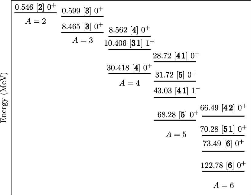
Figure 2: Calculated levels for $A=2-6$ using the all-waves Volkov potential.

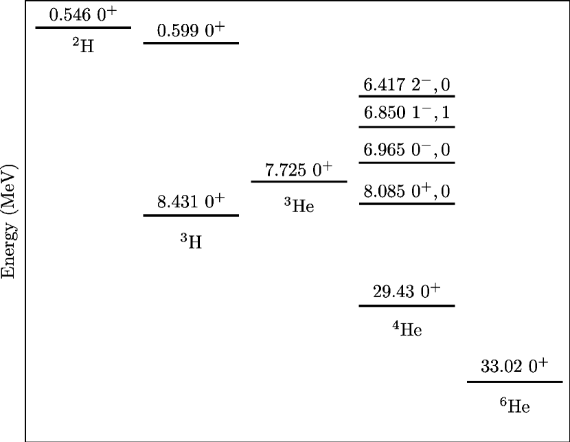
Figure 3: Calculated levels for $A=2,3,4$ and 6, using the $s$-wave Volkov potential with the inclusion of Coulomb interaction for He isotopes. In this case the $A=5$ system results unbounded.

We can conclude that besides its simplicity, the $s$-wave potential describes the $A=4$ system better than the complete potential and, in some cases, in reasonable agreement with the experiment. From a technical point of view we were able to describe the $L=0$ ground and first excited states and the first level of the $L=1$ state using the non-symmetrized HH functions. In particular the convergence of the $L=0$ first excited state, $E_{1}$, presents some difficulties since its energy results to be very close to the threshold. When the Coulomb interaction is taken into account this level moves to the continuum and it appears as a resonance between the two $3+1$ thresholds, in agreement with the experimental data. The $s$-wave potential describes better also the negative parity resonances; moreover, in order to accurately extract their position and width, the present method can be combined with the procedure developed for example in Ref. witala99 . The computed states for $A=3,4$ are collected in Figs. 2,3.

IV.3 $A=5,6$ systems

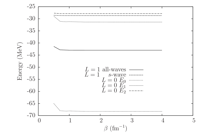
Figure 4: The $A=5$, $L=0$ levels, given in Table 4, denoted as $E_{0},E_{1},E_{2}$ and the $L=1$ levels given in Table 5, denoted as all-waves and s-wave, are shown as functions of the non-linear parameter $\beta$, at $K_{max}=16$ ($L=0$ levels) and $K_{max}=17$ ($L=1$ levels), respectively.

In the case of systems with $A>4$ the spatially-symmetric state cannot be antisymmetrized using the corresponding spin-isospin functions. Therefore, it is interesting to study the symmetry of the different levels in the $A=5$ system when the non-symmetrized basis is used. For the positive parity $L=0$ state, using the Volkov potential, we found that the deepest two levels correspond to a completely symmetric state (the irreducible representation of $S_{5}$ $[\bm{5}]$) as expected. As mentioned, they cannot be antisymmetrized using the spin-isospin functions of five particles and, therefore, they do not represent physical states for five nucleons. The third level belongs to the irreducible representation of $S_{5}$ $[\bm{4\;1}]$; it can be antisymmetrized using the $A=5$ spin-isospin functions having $S=1/2,T=1/2$, and accordingly it represents the lowest level of the $(L,S,T)J^{\pi}=(0,1/2,1/2)1/2^{+}$ state of five nucleons. The convergence of these three states in terms of $K_{max}$ is given in Table 4. The first two levels, representing bosonic bound states, present a good convergence with $K$ (in particular the deepest level). The convergence of the $[\bm{4\;1}]$ state shows that it does not describe a bound state, in agreement with the fact that the $A=5$ nucleus does not exist. In fact its energy results to be above the threshold of $30.42$ MeV describing an ⁴He nucleus plus a fifth nucleon far away (here the Coulomb interaction has not been included). For the three levels, their stability as a function of the non-linear parameter $\beta$ is shown in Fig. 4.

The negative parity $L=1$ state corresponds to the $(L,S,T)J^{\pi}=(1,1/2,1/2)1/2^{-}$ and $(1,1/2,1/2)3/2^{-}$ states which are degenerate using the Volkov potential. Its deepest level cannot be spatially-symmetric, and in fact it belongs to the $[\bm{4\;1}]$ representation; as before, it can be antisymmetrized using the $S=1/2,T=1/2$ spin-isospin functions of five nucleons. In Table 5 the convergence of this level is shown in terms of $K_{max}$ for the all-waves potential as well as its $s$-wave reduction. From the table we can observe that the all-waves version of the potential predicts a very deep bound state, at $43.03$ MeV, whereas the $s$-wave reduction does not. Using the $s$-wave potential, the $A=5$ systems results to be unbounded in agreement with the experimental observation. From this analysis we can conclude that the fact that the $A=5$ nucleus does not exist is the result of a delicate balance between the Pauli principle, the short range character of the NN interaction and its weakness in $p$-waves. The $s$-wave potential, used in the present analysis, represents the extreme case in which the interaction in $p$-waves is considered zero. For these two levels, their stability as a function of the non-linear parameter $\beta$ is shown in Fig. 4 as the solid line (all-waves) and long dashed line (s-wave) respectively. In the last three columns of the table, the three levels obtained considering the $s$-wave Volkov potential plus the Coulomb interaction between two protons are shown. The inclusion of the Coulomb interaction breaks the degeneracy of the quartet-$[\bm{4\;1}]$ state, producing three different states that can be identified by the residual $S_{2}\otimes S_{3}$ symmetry of the two-protons and three-neutrons sub-systems. The lowest two states $E_{0}$ and $E_{1}$ belong to the $[\bm{1}^{2}]\otimes[\bm{3}]$ and $[\bm{2}]\otimes[\bm{3}]$ representations of $S_{2}\otimes S_{3}$ and cannot be antisymmetrized with respect to the three neutrons. The third level, $E_{2}$, is a doublet state since corresponds to a mixed symmetry of the three neutrons and it is symmetric in the two protons. Its belongs to the $[\bm{2}]\otimes[\bm{2\;1}]$ representation and it can be antisymmetrized with the spin state of the two protons having $S_{p}=0$ and the spin state of the three neutrons having $S_{n}=1/2$. Physically this state is describing a scattering state between a neutron and an $\alpha$-particle in $J^{\pi}=1/2^{-}$ and $3/2^{-}$. In the present study we are limiting the description to bound states, however, using the method described in Ref. kievsky10 it would be possible to compute phase-shifts using the $L=0,1$ bound-like states. The extension of the method to describe scattering states is in progress.

In the case of the $A=6$ system we concentrate the analysis in the $(L,S,T)J^{\pi}=(0,0,1)0^{+}$ and $(0,1,0)1^{+}$ states. Using a central potential, and disregarding the Coulomb interaction, these two states are degenerate. Including the Coulomb interaction between two protons, the first state has the quantum numbers of ⁶He. A direct diagonalization of the six body Hamiltonian using the non-symmetrized HH basis, with the Volkov potential, produces a spectrum in which the first two levels belongs to the $[\bm{6}]$ irreducible representation of $S_{6}$. They are completely symmetric and cannot be antisymmetrized using the $A=6$ spin-isospin functions. The third level belongs to the $[\bm{5\;1}]$ representation and it cannot be antisymetrized too. The fourth level belongs to the $[\bm{4\;2}]$ representation, and it is the first one that can be symmetrized using the $A=6$ spin-isospin functions having $S=0,T=1$ or $S=1,T=0$. The convergence pattern of these four levels in terms of $K_{max}$ are shown in Table 6 indicated by $E_{i}$, $i=1,\ldots,4$. Similar to the $A=5$ case, the Volkov potential acting in all waves predicts large binding energies. In particular the binding energy of the physical state results to be $\approx 67$ MeV. Using the $s$-wave potential a much more reasonable value of $\approx 34$ MeV is obtained for this level. The corresponding convergence is shown in the last column of Table 6 indicated by $E^{s}_{3}$. It should be noticed that in the computation of the spectrum using the $s$-wave potential the $E^{s}_{3}$ is not anymore the fourth level. Other levels belonging to the $[\bm{6}]$ and $[\bm{5\;1}]$ representation gain more energy than the $[\bm{4\;2}]$ level, making difficult its correct identification. However, it is possible to restrict the search of the eigenvectors to those having a particular symmetry using a symmetry-adapted Lanczos method slanczos (a description of the iterative method used is given in the Appendix). Essentially, starting with a vector having the desired symmetry, after each iteration of the matrix-vector product, the new vector is projected onto the sub-space of the selected symmetry. Following Ref. slanczos , an intermediate purification step is also implemented. This method has the characteristic of finding eigenvalues corresponding to eigenvectors of one particular symmetry simplifying the search procedure and the identification of the eigenvectors.

When the Coulomb interaction between two protons is considered the degeneracy of the $[\bm{4\;2}]$ level (of dimension 9) is broken and four different states appear. It is possible to identify the physical state looking at the symmetry of the four neutrons. One of the states belongs to the $[\bm{4}]$ representation, two belong to the $[\bm{3\;1}]$ representation and the last one belongs to the $[\bm{2}^{2}]$ representation of $S_{4}$. This last state is the only one that can be antisymmetrized using the spin functions of four neutrons having $S_{n}=0$. Moreover, the proton state is spatially symmetric and therefore can be antisymmetrized with the spin function $S_{p}=0$ making a total $S=0$ state. The convergence of this state is given in the last column of Table 6. It should be noticed that this state is embedded in a very dense spectrum. In order to follow this state in the projected Lanczos method a projection-purification procedure is performed. Essentially the vector, after each matrix vector product, is projected on antisymmetric states between particles (3,4) and (5,6). In this way the level belonging to the $[\bm{2}]\otimes[\bm{2}^{2}]$ representation of $S_{2}\otimes S_{4}$ results to be the lowest one. The results obtained for the different levels are collected in Figs. 2,3.

V Conclusions

In this work we have developed a technique devoted to describe bound states in an $A$-body system without imposing a particular requirement due to the intrinsic statistic of the particles. However, the final aim of the method is to found wave functions that fulfill this requirement.

Starting with the non-symmetrized HH basis set, we have diagonalized the Hamiltonian of the $A$-body system using that basis at fixed values of $K$. We have observed that the eigenvectors reflect the symmetries present in the Hamiltonian and, in particular, if the system is composed by identical particles, the eigenvectors belong to the different irreducible representations of the permutation group of $A$ objects, $S_{A}$. Using a Casimir operator, it was possible to identify those eigenvectors having the required symmetry of the system and, accordingly, study the convergence (in terms of $K$) of the corresponding eigenvalues. The direct use of the non-symmetrized HH basis has important consequences from a technical point of view. The size of the basis is much bigger than the one limited to a subspace having a particular symmetry. However, it should be noticed that a system of nucleons includes spatial, spin and isospin degrees of freedom, all of them coupled by the NN potential, with the consequence that different spatial symmetries are present in an $A$-nucleon wave function. Although the construction of HH basis elements having different spatial symmetries is possible (see for example Ref. barnea99 ), the necessity of including the different symmetries in the description enlarges the dimension of the basis and makes it comparable to the case in which the non-symmetrized basis is used. This is particularly important when one wants to consider the description of the small components of the wave function induced by symmetry breaking terms in the potential, as for example high isospin components.

The method here presented is based in a particular implementation of the potential energy matrix constructed as a sum of products of sparse matrices. This allows to efficiently use iterative algorithms in which the matrix-vector product is a key element. However the iterative methods are well suited to calculate the deepest levels of the spectrum. In our formulation, due to the presence of different symmetries, the physical states could appear very high in the spectrum or in a zone with a high density of levels. In this case we found very convenient to use the symmetry-adapted Lanczos method slanczos . Using the particular form of the permutation operator $P(i,j)$ in terms of the sparse matrices (see Eq.(48)), it was possible to project the vector in the iterative procedure to be antisymmetric in selected pairs of particles. In this way the desired symmetry becomes the lowest state of the spectrum. Though this mechanism is not as fast as searching for the true lowest state of the complete spectrum, it is much faster than searching for certain numbers of levels in high position of the spectrum.

We should also stress that the sparse matrices ${}^{(i)}{\cal A}$ defined in Eq.(31) have the property of being constructed as products of the angular $T$-coefficients, the tree ${\cal T}$-coefficients and the Raynal-Revai coefficients. Whereas the latters couples quantum number belonging to the $[K]$ and $[K^{\prime}]$ sets, the $T$- and ${\cal T}$-coefficients perform a recoupling of quantum numbers inside $[K]$ or $[K^{\prime}]$. Moreover the Raynal-Revai coefficients ${\cal R}^{K,L}_{l_{2}l_{1},l^{\prime}_{2}l^{\prime}_{1}}$ couple quantum numbers belonging to three particles (see Eq.(29)). As the number of particles $A$ increases, more values of the quantum numbers $K,L$ are accessible and this makes the size of the ${}^{(i)}{\cal A}$ matrices to increase, though slowly with the number of particles $A$. Furthermore, going from a system with $A$ particles to $A+1$, the number of potential terms increase by $A$ and the number of factors in the matrix ${\cal B}_{ij}^{LM}$ of Eq.(34) increases at maximum of the same quantity. The computational effort increases roughly linear with $A$ and this fact makes feasible the application of the method for increasing values of $A$ as has been demonstrated in the present work. Our expectation is that the present technique could be extended to treat systems up to $A=8$. The calculations presented here have been obtained using a sequential code. We expect that an opportune parallelization of the code (which is under study) will increase the potentiality of the method.

We have limited the analysis to consider a central potential, the Volkov potential, used several times in the literature. Though the use of a central potential leads to an unrealistic description of the light nuclei structures, the study has served to analyze the characteristic of the method: the capability of the diagonalization procedure to construct the proper symmetry of the state and the particular structure, in terms of products of sparse matrices, of the Hamiltonian matrix. The success of this study makes feasible the extension of the method to treat interactions depending on spin and isospin degrees of freedom as the realistic NN potentials. A preliminary analysis in this direction has been done mario09 . To this respect it is important to notice that the information of the potential is given in the matrix $V_{12}$ defined in Eq.(37). Once this matrix is given, the method remains the same, with the basis enlarged to include spin and isospin degrees of freedom if required. Using the Volkov potential we have shown that it was possible to identify all the physical states and the corresponding thresholds in order to interpret the level as bounded or belonging to the continuum. Furthermore, the results obtained using the Volkov potential up to $A=6$ compare well with other techniques. A few characteristic of the $A=3-6$ systems using the Volkov potential are the following. Due to its particular parametrization a shallow state appears in the $A=3,4$ systems when the Coulomb interaction is not considered. In the $A=3$ this state has the characteristic of an Efimov state. When the Coulomb interaction is considered these states move to the continuum. The Volkov potential acting in all waves produces large binding energies as $A$ increases. Accordingly we have included in the analysis the $s$-wave version of the potential. In agreement with the experimental observations, this version predicts in reasonable positions the $A=4$ $0^{+}$ and $0^{-}$ resonances and no bound states in the $A=5$ system. It also predicts reasonable binding energies in the $A=6$ system. The extension of the method to consider realistic potentials is in progress.

VI Appendix

The diagonalization of the Hamiltonian is obtained by means of an iterative algorithm which requires only the action of the Hamiltonian matrix on a given vector. We used the Lanczos algorithm in the version invented by Cullum and Willoughby cullum which is particularly sparing with memory use. In principle, the iterative procedure should preserve the permutation symmetry of the input vector, as the Hamiltonian commutes with the group elements. However, the round-off errors generate components also in the other irreducible representations. To circumvent this problem, we have used a symmetry adapted Lanczos (SAL) developed in Ref. slanczos in which a projection operator is applied after each iterative step. Starting from a random initial vector, in the usual Lancsoz recurrence formula

$$\beta_{i+1}{\bm{v}}_{i+1}=H{\bm{v}}_{i}-\alpha_{i}{\bm{v}}_{i}-\beta_{i}{\bm{v}}_{i-1}\,,$$ (50)

the product $H{\bm{v}}_{i}$ is replaced by $P^{[{\widehat{\bm{\lambda}}}]}H{\bm{v}}_{i}$, where $P^{[\widehat{\bm{\lambda}}]}$ is a projector on a sub-space with a non-zero intersection with the irreducible representation $[{\bm{\lambda}}]$, and zero intersection with the irreducible representations of the lower-eigenvector symmetries. A purification step is also performed in which the product $\beta_{i+1}{\bm{v}}_{i+1}$ is replaced by $P^{[\widehat{\bm{\lambda}}]}\beta_{i+1}{\bm{v}}_{i+1}$.

As an example in the $L=0$ sector of the $A=6$ system, we are interested in states belonging to the irreducible representation $[{\bm{4}\,\bm{2}}]$. In order to eliminate lower states belonging to the irreducible representations $[{\bm{6}}]$ and $[{\bm{5}\,\bm{1}}]$, we have used the projector

$$P^{\widehat{[{\bm{4}\;\bm{2}}]}}=A_{12}\cdot A_{34}\,,$$ (51)

given as the product of the antisymmetrization operator $A_{12}$ with respect particles $(1,2)$, and the antisymmetrization operator $A_{34}$ with respect particles $(3,4)$. The two antisymmetrization operators have the following expression in terms of the ${\cal A}_{i}$ matrices (the superscript $L,M=0,0$ is understood)

$$A_{12}=\frac{1}{2}(1-{\cal A}_{5}),$$ (52)

and

$$A_{34}={\cal A}_{4}{\cal A}_{3}{\cal A}_{4}\,\frac{1-{\cal A}_{5}}{2}\,{\cal A}_{4}{\cal A}_{3}{\cal A}_{4}\,.$$ (53)

Table 1: $A=3$ results for $(L,S,T)J^{\pi}=(0,\frac{1}{2},\frac{1}{2})\frac{1}{2}^{+}$ state using the all-waves and $s$-wave Volkov potential as a function of the maximum grand angular quantum number $K_{max}$. The ground state $E_{0}$ as well as the excited state $E_{1}$ are shown.

	all-waves		$s$-wave
$K_{max}$	$E_{0}$ (MeV)	$E_{1}$ (MeV)	$E_{0}$ (MeV)	$E_{1}$ (MeV)
20	8.4623	0.3627	8.4283	0.3618
40	8.4649	0.5181	8.4309	0.5174
60	8.4649	0.5595	8.4309	0.5589
80	8.4649	0.5773	8.4309	0.5768
100		0.5866		0.5861
120		0.5918		0.5913
140		0.5947		0.5943
160		0.5965		0.5960
180		0.5976		0.5971
200		0.5982		0.5978
240		0.5989		0.5985
280		0.5992		0.5988
320		0.5993		0.5989
SVM varga95	8.46
Ref. barnea99	8.462	0.2599

Table 2: Binding energies for the $A=4$ ground state $E_{0}$ and the first excited state $E_{1}$ of the $(L,S,T)J^{\pi}=(0,0,0)0^{+}$ state using the all-waves and $s$-wave Volkov potentials as a function of the maximum grand angular quantum number $K_{max}$. In the last four columns the Coulomb interaction has been considered. For the sake of comparison the results of Refs. barnea99 ; varga95 are shown.

	all-waves		$s$-wave		all-waves		$s$-wave
$K_{max}$	$E_{0}$ (MeV)	$E_{1}$ (MeV)	$E_{0}$ (MeV)	$E_{1}$ (MeV)	$E_{0}$ (MeV)	$E_{1}$ (MeV)	$E_{0}$ (MeV)	$E_{1}$ (MeV)
0	28.580	3.238	28.580	3.238	27.748	2.787	27.748	2.787
10	30.278	7.509	30.116	7.445	29.456	7.039	29.292	6.976
20	30.416	8.223	30.250	8.164	29.596	7.778	29.429	7.720
30	30.418	8.463	30.252	8.403	29.599	8.035	29.431	7.976
40	30.418	8.562	30.252	8.501	29.600	8.144	29.432	8.085
SVM varga95	30.42
Ref. barnea99	30.406	8.036

Table 3: The binding energy of the $A=4$ lowest level having $L=1$, using the all-waves and $s$-wave Volkov potential, as a function of the maximum grand angular quantum number $K_{max}$. In the case of $s$-wave potential, when Coulomb interaction between particles (1,2) is considered, the level splits in three sub-levels, whose energies $E_{0}$, $E_{1}$ and $E_{2}$ are shown in the last three columns.

$K_{max}$	all-waves	$s$-wave	$E_{0}$ (MeV)	$E_{1}$ (MeV)	$E_{2}$ (MeV)
1	7.965	0.387	-	-	-
3	8.411	1.975	1.639	1.440	1.374
11	10.121	5.567	5.314	5.091	4.899
21	10.373	6.642	6.456	6.276	5.955
31	10.406	7.113	6.965	6.850	6.417

Table 4: $A=5$ binding energies of the first three levels of the $L=0$ state, belonging to the indicated irreducible representation $[\bm{\lambda}]$, as a function of $K_{max}$. The size of the HH basis $N_{HH}$ is also indicated.

$K_{max}$	$N_{HH}$	$E_{0}$ (MeV)	$E_{1}$ (MeV)	$E_{2}$ (MeV)
		[$\bm{5}$]	[$\bm{5}$]	[$\bm{4\;1}$]
0	1	64.864	24.472	-
2	10	64.864	24.472	20.160
4	55	65.958	28.411	22.043
6	220	66.893	29.517	24.415
8	714	67.713	30.228	25.568
10	1992	68.008	30.587	26.459
12	4950	68.177	30.927	27.043
14	11220	68.239	31.152	27.515
16	23595	68.264	31.357	27.862
18	46618	68.274	31.509	28.143
20	87373	68.278	31.628	28.371
22	156520	68.279	31.715	28.560
24	269620	68.280	31.779	28.719

Table 5: $A=5$ binding energies of the deepest $L=1$ state, as a function of $K_{max}$, using the all-waves and $s$-wave Volkov potential. In the last three columns the Coulomb potential has been summed to the $s$-wave Volkov potential. The size of the HH basis $N_{HH}$ is also indicated.

$K_{max}$	$N_{HH}$	all-waves	$s$-wave	$E_{0}$	$E_{1}$	$E_{2}$
1	4	39.635	21.874	21.370	21.119	-
3	40	40.001	24.317	23.854	23.604	23.524
5	220	41.022	26.053	25.618	25.367	25.251
7	876	41.785	26.923	26.505	26.258	26.116
9	2820	42.384	27.546	27.140	26.896	26.736
11	7788	42.682	27.971	27.574	27.333	27.160
13	19140	42.868	28.297	27.908	27.669	27.485
15	42900	42.952	28.521	28.140	27.903	27.710
17	89232	42.996	28.693	28.320	28.084	27.882
19	174460	43.017	28.823	28.457	28.223	28.011
21	323752	43.027	28.924	28.562	28.331	28.110
23	574600	43.032	29.005	28.647	28.417	28.189
SVM		43.00
HH barnea99		42.383

Table 6: $A=6$ binding energies of the first four levels of the $L=0$ state, using the Volkov potential, belonging to the indicated irreducible representation $[\bm{\lambda}]$, as a function of $K_{max}$. $E^{s}_{3}$ indicates the binding energy of the lowest [$\bm{4\;2}$] state using the $s$-wave Volkov potential, and $E_{3}^{sc}$ is the binding energy of the $[\bm{2}]\otimes[\bm{2^{2}}]$ state, once the Coulomb interaction has been included. The size of the HH basis $N_{HH}$ is also indicated.

$K_{max}$	$N_{HH}$	$E_{0}$ (MeV)	$E_{1}$ (MeV)	$E_{2}$ (MeV)	$E_{3}$ (MeV)	$E_{3}^{s}$ (MeV)	$E_{3}^{sc}$ (MeV)
		[$\bm{6}$]	[$\bm{6}$]	[$\bm{5\;1}$]	[$\bm{4\;2}$]	[$\bm{4\;2}$]	$[\bm{2}]\otimes[\bm{2^{2}}]$
0	1	117.205	64.701	-	-	-	-
2	15	117.205	64.701	62.513	61.142	24.793	24.064
4	120	118.861	69.450	64.277	62.015	28.791	28.016
6	680	120.345	70.544	66.268	63.377	30.723	29.935
8	3045	121.738	71.443	67.280	64.437	31.645	30.851
10	11427	122.317	71.923	68.371	65.354	32.244	31.446
12	37310	122.597	72.477	69.029	65.886	32.708	31.908
14	108810	122.711	72.822	69.531	66.201	33.075	32.275
16	288990	122.752	73.101	69.842	66.360	33.358	32.558
18	709410	122.768	73.284	70.051	66.437	33.561	32.762
20	1628328	122.774	73.407	70.189	66.474	33.710	32.912
22	3527160	122.776	73.485	70.283	66.491	33.814	33.017
SVM					66.25

Figure 1: Hyperspherical tree corresponding to Eq.( 7)

References

- (1) S.C. Pieper, K. Varga, and R.B. Wiringa, Phys. Rev. C66, 044310 (2002).
- (2) P. Navrátil, V.G. Gueorguiev, J.P. Vary, W.E. Ormand, and A. Nogga, Phys. Rev. Lett. 99, 042501 (2007).
- (3) A. Kievsky et al., Phys. Rev. C58, 3085 (1998).
- (4) R. Lazauskas et al., Phys. Rev. C71, 034004 (2005).
- (5) H. Kamada et al., Phys. Rev. C64, 044001 (2001).
- (6) A. Novoselsky and J. Katriel, Phys. Rev A 49, 833 (1994).
- (7) A. Novoselsky and N. Barnea, Phys. Rev A 51, 2777 (1995).
- (8) N. Barnea, Phys. Rev. A 59, 1135 (1999).
- (9) N. K. Timofeyuk, Phys. Rev. C 78, 054314 (2008).
- (10) M. Gattobigio, A. Kievsky, M. Viviani, and P. Barletta, Phys. Rev A 79, 032513 (2009).
- (11) M. Viviani, A. Kievsky, and S. Rosati, Phys. Rev. C 71, 024006 (2005).
- (12) Xiao-Gang Wang and Tucker Carrington, Jr, J. Chem. Phys. 114, 1473 (2001)
- (13) N. Ya. Vilenkin, G. I. Kuznetsov, and Ya. A. Smorodinskii, Sov. J. Nucl. Phys. 2, 645 (1966).
- (14) M.S. Kil’dyushov, Yad. Fiz. 15, 197 (1972) [Sov. J. Nucl. Phys. 15, 113 (1972)]
- (15) M.S. Kil’dyushov, Yad. Fiz. 16, 217 (1972) [Sov. J. Nucl. Phys. 16, 117 (1973)]
- (16) N. Barnea and A. Novoselsky, Ann. of Phys.256, 192 (1997).
- (17) J. Raynal and J. Revai, Nuovo Cimento A 68, 612 (1970).
- (18) R. Krivec and V.B. Mandelzweig, Phys. Rev. A 42, 3779 (1990).
- (19) M. Viviani, Few-Body Syst. 25, 177 (1998).
- (20) V.D. Efros, Few-Body Syst. 19, 167 (1995).
- (21) K. Varga and Y. Suzuki, Phys. Rev. C 52, 2885 (1995).
- (22) N. K. Timofeyuk, Phys. Rev. C 65, 064306 (2002).
- (23) A. Novoselsky and J. Katriel, Phys. Rev C 51, 412 (1995).
- (24) E. Braaten and H.-W. Hammer, Phys. Rept. 428, 259 (2006)
- (25) P. Barletta and A. Kievsky, Few-Body Syst.45, 25 (2009)
- (26) P. Barletta, C. Romero-Redondo, A. Kievsky, M. Viviani, and E. Garrido, Phys. Rev. Lett. 103, 090402 (2009)
- (27) P. Barletta and A. Kievsky, Phys. Rev. A 64, 042514 (2001)
- (28) A. Kievsky et al., Phys. Lett. B 406, 292 (1997)
- (29) D.R. Tilley, H.R. Weller and G.M. Hale, Nuc. Phys. A 541, 1 (1992)
- (30) H. Witała and W. Glöckle, Phys. Rev. C 60, 024002 (1999)
- (31) A. Kievsky, M. Viviani, P. Barletta, C. Romero-Redondo, and E. Garrido, Phys. Rev. C 81, 034002 (2010)
- (32) M. Gattobigio, A. Kievsky, M. Viviani, and P. Barletta, Few-Body Syst. 45, 127 (2009)
- (33) J. K. Cullum and R. A. Willoughby, J. Comput. Phys. 44, 329 (1981)