Cosmological and Solar-System Tests of $f(R)$ Modified Gravity

Abstract

We investigate the cosmological and the local tests of the $f(R)$ theory of modified gravity via the observations of (1) the cosmic expansion and (2) the cosmic structures and via (3) the solar-system experiments. To fit the possible cosmic expansion histories under consideration, for each of them we reconstruct $f(R)$, known as “designer $f(R)$”. We then test the designer $f(R)$ via the cosmic-structure constraints on the metric perturbation ratio $\Psi/\Phi$ and the effective gravitational coupling $G_{\textrm{eff}}$ and via the solar-system constraints on the Brans-Dicke theory with the chameleon mechanism. We find that among the designer $f(R)$ models specified by the CPL effective equation of state $w_{\textrm{eff}}$, only the model closely mimicking general relativity with a cosmological constant ($\Lambda$CDM) can survive all the tests. Accordingly, these tests rule out the frequently studied $w_{\textrm{eff}}=-1$ designer $f(R)$ models which are distinct in cosmic structures from $\Lambda$CDM. When considering only the cosmological tests, we find that the surviving designer $f(R)$ models, although exist for a variety of $w_{\textrm{eff}}$, entail fine-tuning.

I Introduction

Our universe is presently at the stage of accelerating expansion, as suggested by the cosmological observations Perlmutter:1998np ; Riess:1998cb . Assuming a homogeneous and isotropic universe and based on general relativity (GR), one cannot explain this late-time cosmic acceleration if the universe contains only matter and radiation. A substance with negative pressure adding to the right-hand side of the Einstein field equations, known as dark energy Huterer:1998qv , can lead to the cosmic acceleration DEreview . Observations Komatsu:2010fb ; Kowalski:2008ez ; Eisenstein:2005su suggest that our universe should be nearly flat and consist of 73% dark energy, 22% dark matter, 5% ordinary matter, and approximated 0.008% radiation. It is ironic that so far our knowledge of physics can only explain 5% of the universe, with nearly 95% of the universe remained unexplained. This is the most challenging issue for the physicists of the 21st century.

Instead of invoking dark energy, there have been attempts to modify the left-hand side of the Einstein equations, e.g. via proposing alternative gravity theories, to explain the late-time acceleration Dvali:2000hr ; Maartens:2003tw ; Bekenstein:2004ne ; Jacobson:2000xp (see Nojiri:2006ri for a review). These attempts are known as modified gravity. Among these theories, in the present paper we will focus on the $f(R)$ theory of modified gravity where the Einstein-Hilbert Lagrangian density is added by a general function of the Ricci scalar, $f(R)$.

A. A. Starobinsky was the first to point out that de Sitter space, and therefore the exponential expansion of spacetime, can be achieved in the early universe by quantum correction, ($R+\alpha^{2}R^{2}$), to the Einstein-Hilbert action Starobinsky:1980te . This UV modification leads to an early accelerating universe (Starobinsky inflation) and motivates people to construct the $f(R)$ models Capozziello:2003tk ; Carroll:2003wy to explain the late-time acceleration of the universe. Since the $f(R)$ theory is equivalent to the Brans-Dicke theory with the Brans-Dicke parameter $\omega_{\textrm{BD}}=0$ Chiba:2003ir , it seems that this is already ruled out by the constraint $\omega_{\textrm{BD}}>4\times 10^{4}$ set by observations Will:2001mx ; Bertotti:2003rm ; Will:2005va . Nevertheless, it was pointed out recently that in a non-minimally coupled scalar-tensor theory the scalar field may have a scale- or environment-dependent mass via its interaction with matter Khoury:2003aq ; Khoury:2003rn . That is, the higher (lower) the matter density is, the more (less) massive the scalar field is. Consequently, in the solar system, which has a much higher density than the universe, the scalar field would have a large effective mass (and therefore a small Compton wavelength) so that it can evade the solar-system tests. At the mean time, the same scalar field would have a much smaller effective mass at cosmological scales, as small as the present Hubble expansion rate (i.e. a long Compton wavelength comparable to the size of the universe). Accordingly, it can be a candidate driving the late-time cosmic acceleration. The sensitivity to the environment of such a scalar field interaction gives the name, “chameleon mechanism” Khoury:2003aq ; Khoury:2003rn .

In this paper we investigate various tests of the $f(R)$ theory of modified gravity. As an alternative to dark energy for driving the late-time cosmic acceleration, the $f(R)$ theory needs to pass the cosmological tests, including the constraints about (1) the cosmic expansion and (2) the cosmic structure formation. In addition, as a modified gravity theory, it needs to pass (3) the solar-system test, such as the constraints on the Brans-Dicke theory. The process of these three tests in the present paper are described in the following.

(1) Cosmic Expansion History: For the background cosmic expansion there is a degeneracy between $f(R)$ modified gravity and GR with dark energy, that is, one cannot distinguish between these two theories via the observations about the cosmic expansion history such as type Ia supernovae (SNIa) and baryon acoustic oscillations (BAO). This is because for any given expansion history $H(t)$ one can always construct a function $f(R)$ to generate the required expansion. The $f(R)$ model so constructed is called “designer $f(R)$” Pogosian:2007sw . To fit the observational constraint on $H(t)$, we take the designer $f(R)$ approach to (re)construct $f(R)$ for possible expansion histories, where $f(R)$ is specified by $H(t)$ and the initial condition, particularly the value of $df/dR$ at some initial time, as denoted by $f_{Ri}$. In the present paper we consider the expansion history $H(t)$ given by the effective dark energy equation of state $w_{\textrm{eff}}$ as specified by the Chevallier-Polarski-Linder (CPL) parametrization Chevallier:2000qy ; Linder:2002et , $w_{\textrm{CPL}}=w_{0}+w_{a}z/(1+z)$ (where $z$ is redshift), with the current observational constraints on $w_{0}$ and $w_{a}$ Komatsu:2010fb . In this case the designer $f(R)$ is parametrized by three parameters, $\{w_{0},w_{a},f_{Ri}\}$. We then test such designer $f(R;\{w_{0},w_{a},f_{Ri}\})$ model via the cosmic-structure observations and the solar-system experiments.

(2) Cosmic Structure Formation: For each designer $f(R;\{w_{0},w_{a},f_{Ri}\})$ obtained above we calculate the theoretical prediction of the cosmological perturbations, particularly $\Psi/\Phi$ and $G_{\textrm{eff}}/G_{N}$ at late times and at subhorizon scales, where $\Psi$ and $\Phi$ are two metric potentials in the Newtonian gauge, and $G_{\textrm{eff}}$ and $G_{N}$ are the effective gravitational coupling and the Newtonian constant, respectively. In GR these two ratios are both unity, while in $f(R)$ modified gravity they generally change with time and scales. For the test we compare the theoretical prediction with the observational requirements from the cosmic structure observations, thereby constraining $f(R;\{w_{0},w_{a},f_{Ri}\})$, i.e., obtaining the constraints on the parameter space $\{w_{0},w_{a},f_{Ri}\}$. In particular, we obtain the allowed range of $f_{Ri}$ for various $\{w_{0},w_{a}\}$ under consideration.

(3) Solar-system Tests: The solar-system experiments provide stringent constraints on the Brans-Dicke theory with the chameleon mechanism, and accordingly tightly constrain the behavior of $f(R)$ for $R/H_{0}^{2}\gtrsim 10^{5}$ Faulkner:2006ub ; Capozziello:2007eu ; Bisabr:2009ee ; Gu:2010 . To do the solar-system test, for each designer $f(R;\{w_{0},w_{a},f_{Ri}\})$ we check whether it is consistent with this constraint on $f(R/H_{0}^{2}\gtrsim 10^{5})$.

Through the above three tests we find that only the models which closely mimic GR with a cosmological constant can survive these three tests. That is, among the $f(R;\{w_{0},w_{a},f_{Ri}\})$ models under consideration, only the case where $f(R)\simeq\textrm{constant}$ or $\{w_{0},w_{a},f_{Ri}\}$ very close to $\{-1,0,0\}$ survives these three tests. For comparison, when we consider only the cosmological tests, i.e. the tests (1) and (2), for each $\{w_{0},w_{a}\}$ under consideration we find the allowed range of $f_{Ri}$ very narrow although existing. This presents a severe fine-tuning of the initial condition of $f(R)$ for passing the cosmological tests.

This paper is organized as follows. In Sec. II we introduce the basics of the background evolution in the $f(R)$ theory, the construction of the designer $f(R)$ models, and the evolution of the cosmological perturbations with the late-time and the subhorizon approximations. In Sec. III we introduce the observational constraints set by the observations about the cosmic expansion and the cosmic structures and by the solar-system experiments. In Sec. IV we show the results of the three tests. We then conclude in Sec. V.

II Basics of $f(R)$ Modified Gravity

II.1 Background evolution

We start with the following modified Hilbert-Einstein action for the $f(R)$ theory of modified gravity.

$$S=\frac{1}{2\kappa^{2}}\int d^{4}x\sqrt{-g}~{}\left[R+f(R)\right]+\sum_{\scriptstyle{a}}S_{a}\ ,$$ (1)

where $f(R)$ is a general function of the Ricci scalar and represents the deviation from GR, and $S_{a}$ with $a=r,m$ are the actions for radiation and matter (including dark matter and baryons), respectively. The variation of this action with respect to the metric tensor gives the gravitational field equations,

$$G_{\mu\nu}+\left(f_{R}R_{\mu\nu}-\frac{1}{2}fg_{\mu\nu}\right)+\left(g_{\mu\nu}\square-\nabla_{\mu}\nabla_{\nu}\right)f_{R}$$

$$=\kappa^{2}T_{\mu\nu}=\kappa^{2}\sum_{\scriptstyle{a}}T^{(a)}_{\mu\nu}\ ,$$ (2)

where the d’Alembertian operator $\square\equiv\nabla_{\nu}\nabla^{\nu}$, $f_{R}\equiv df/dR$, likewise $f_{RR}\equiv d^{2}f/dR^{2}$, and the energy-momentum tensor of the cosmic fluid $T^{(a)}_{\mu\nu}\equiv-(2/\sqrt{-g})(\delta S^{(a)}/\delta g^{\mu\nu})$.

Regarding the background evolution, we consider the flat Robertson-Walker metric for describing the background space-time,

$$ds^{2}=-dt^{2}+a^{2}(t)d\vec{x}~{}^{2}\ ,$$ (3)

and the perfect fluids for the energy contents,

$$T^{\mu}_{~{}\,\nu}=\sum_{a}diag(-\rho_{a},p_{a},p_{a},p_{a}),$$ (4)

where $\rho_{a}$ and $p_{a}$ are the energy density and pressure. We then obtain two evolution equations describing the cosmic expansion:

$$H^{2}+\frac{1}{6}f+\left(H^{2}-\frac{1}{6}R\right)f_{R}+H\dot{f_{R}} = \frac{\kappa^{2}}{3}\left(\rho_{m}+\rho_{r}\right),$$ (5)

$$\frac{\ddot{a}}{a}+\frac{1}{6}f-H^{2}f_{R}+\frac{1}{2}H\dot{f_{R}}+\frac{1}{2}\ddot{f_{R}} = \frac{-\kappa^{2}}{6}\left(\rho_{m}+2\rho_{r}\right),$$ (6)

where an over-dot denotes the derivative with respect to the cosmic time $t$, the Hubble expansion rate $H=\dot{a}/a$, the Ricci scalar $R=6\dot{H}+12H^{2}$, and we have used $p_{m}=0$ and $p_{r}=\rho_{r}/3$. Equation (6) shows that matter and radiation can simply contribute to deceleration, while the deviation from GR may induce accelerated expansion when its contribution therein, $f/6-H^{2}f_{R}+H\dot{f_{R}}/2+\ddot{f_{R}}/2$, is negative and significant. In addition, from these equations one can see that the $f(R)$ theory comes back to GR (with a cosmological constant $\Lambda$) at the background level when $f(R)=\textrm{constant}=-2\Lambda$.

The above two equations can be recast in the form in GR:

$$H^{2} = \frac{\kappa^{2}}{3}\left(\rho_{m}+\rho_{r}+\rho_{\textrm{eff}}\right),$$ (7)

$$\frac{\ddot{a}}{a} = -\frac{\kappa^{2}}{6}\left(\rho_{m}+2\rho_{r}+\rho_{\textrm{eff}}+3p_{\textrm{eff}}\right).$$ (8)

Here $\rho_{\textrm{eff}}$ and $p_{\textrm{eff}}$ are respectively the effective energy density and the effective pressure contributed from the deviation from GR, $f(R)$, and are defined as

$$\rho_{\textrm{eff}} \equiv \frac{1}{\kappa^{2}}\left[-\frac{1}{2}f-3\left(H^{2}-\frac{1}{6}R\right)f_{R}-3H\dot{f_{R}}\right],$$ (9)

$$p_{\textrm{eff}} \equiv \frac{1}{\kappa^{2}}\left[\frac{1}{2}f-\left(H^{2}+\frac{R}{6}\right)f_{R}+2H\dot{f_{R}}+\ddot{f_{R}}\right].$$ (10)

This effective energy density satisfies the conservation equation,

$$\dot{\rho}_{\textrm{eff}}=-3H\left(1+w_{\textrm{eff}}\right)\rho_{\textrm{eff}}\,,$$ (11)

where

$$w_{\textrm{eff}}\equiv p_{\textrm{eff}}/\rho_{\textrm{eff}}\,.$$ (12)

For a given expansion history $H(t)$ and given energy densities, $\rho_{m}(t)$ and $\rho_{r}(t)$, Eq. (5) gives a second-order differential equation for $f(R)$ or $f(t)$, with the understanding that $f_{R}=\dot{f}/\dot{R}$ and $\dot{f}_{R}=\ddot{f}/\dot{R}-\ddot{R}\dot{f}/\dot{R}^{2}$. Equivalently, for a given effective energy density $\rho_{\textrm{eff}}$ that together with $\rho_{m}$ and $\rho_{r}$ specifies the expansion history, Eq. (9) gives the same differential equation for $f(R)$ Pogosian:2007sw :

$$\frac{f^{\prime\prime}}{H^{2}_{0}}-\left(1+\frac{E^{\prime}}{2E}+\frac{R^{\prime\prime}}{R^{\prime}}\right)\frac{f^{\prime}}{H^{2}_{0}}$$ (13)

$$+\left(\frac{12E^{\prime}}{E}+\frac{3E^{\prime\prime}}{E}\right)\left(\frac{f}{6H^{2}_{0}}+E_{\textrm{eff}}\right)=0,$$

where the prime denotes the derivative with respect to $\ln a$, and

$$E(a) \equiv H^{2}/H^{2}_{0}=\Omega_{m}a^{-3}+\Omega_{r}a^{-4}+E_{\textrm{eff}},$$ (14)

$$E_{\textrm{eff}}(a) \equiv \rho_{\textrm{eff}}/\rho_{c}=\Omega_{\textrm{eff}}\exp\left\{-3\int_{0}^{\ln a}\left[1+w_{\textrm{eff}}(\tilde{a})\right]d\ln\tilde{a}\right\}.$$ (15)

Here the density fraction $\Omega_{i}\equiv\rho_{i}(\textrm{now})/\rho_{c}$ (for $i=m,r,\textrm{eff}$), $\rho_{c}$ is the present critical density, and $\Omega_{m}+\Omega_{r}+\Omega_{\textrm{eff}}=1$ under our consideration of a flat universe. Accordingly, the function $f(R)$ which satisfies this differential equation can generate the required expansion history. Since in general the solution of this differential equation exists (and is not unique), for any given expansion history there always exists a function $f(R)$ which can generate that required expansion. As a result, we cannot distinguish between $f(R)$ modified gravity and dark energy via the observations about the cosmic expansion.

II.2 Designer $f(R)$

In the study of $f(R)$ modified gravity, one may start with a carefully chosen function $f(R)$. On the other hand, one may instead reconstruct $f(R)$ from a given expansion history (together with the information about the energy contents), i.e., considering the solutions $f$ of Eq. (13) for given cosmological parameters $\{H_{0},\Omega_{m},\Omega_{r},\Omega_{\textrm{eff}}\}$ and given $w_{\textrm{eff}}(a)$. The $f(R)$ so constructed is called “designer $f(R)$” Pogosian:2007sw . This phenomenological approach makes sense particularly when one expects that the future cosmological observations will give precise and detailed information about the cosmic expansion.

Solving Eq. (13) requires initial conditions, with different setting of which one obtains different solution $f(R)$. Thus, the designer $f(R)$ is in general a functional of $\{H_{0},\Omega_{m},\Omega_{r},\Omega_{\textrm{eff}}\}$, $w_{\textrm{eff}}(a)$ and the initial conditions. In the present paper we will fix $\{H_{0},\Omega_{m},\Omega_{r},\Omega_{\textrm{eff}}\}$, while consider a variety of $w_{\textrm{eff}}(a)$ and initial conditions for possible $f(R)$.

It has been shown Pogosian:2007sw that the two initial conditions originally needed for solving the second-order differential equation (13) can be simplified to only one condition. This is done as follows. At the early times we require the deviation for GR be tiny in order to satisfy the stringent constraints about cosmic microwave background (CMB) and big-bang nucleosynthesis (BBN), and therefore $\rho_{\textrm{eff}}\ll\rho_{r,m}$. With this approximation, one can obtain an analytic solution of Eq. (13), which is the sum of a particular solution and a growing-mode and a decaying mode homogeneous solutions with two arbitrary constants to be determined by two initial conditions. Since the decaying mode entails a large deviation from GR at early times and cannot fit the above-mentioned requirement, one may exclude the decaying-mode homogeneous solution. Then only one arbitrary constant remains and only one initial condition is needed. The initial conditions for $f$ and $f^{\prime}$ at an initial time $a_{i}$ can be specified as follows Pogosian:2007sw .

$$\frac{f_{i}}{H^{2}_{0}} \simeq A_{+}a_{i}^{p_{+}}+A_{p}E_{\textrm{eff}}(a_{i})\,,$$ (16)

$$\frac{f^{\prime}_{i}}{H^{2}_{0}} \simeq p_{+}A_{+}a_{i}^{p_{+}}-3\left[1+w_{\textrm{eff}}(a_{i})\right]A_{p}E_{\textrm{eff}}(a_{i})\,,$$ (17)

where

$$A_{p} = \frac{-6c}{-3w^{\prime}_{\textrm{eff}}(a_{i})+9w^{2}_{\textrm{eff}}(a_{i})+\left(18-3b\right)w_{\textrm{eff}}(a_{i})+9-3b+c}\,,$$

$$p_{+} = \frac{-b+\sqrt{\,b^{2}-4c}}{2}\,,$$

$$b \equiv \frac{7+8r}{2\left(1+r\right)}~{},~{}c\equiv\frac{-3}{2\left(1+r\right)}\,,$$

$$r \equiv \frac{a_{eq}}{a_{i}}=\frac{1}{a_{i}}\frac{\Omega_{r}}{\Omega_{m}}\,.\$$

The remaining one arbitrary constant is the amplitude of the growing-mode homogeneous solution, $A_{+}$. Instead of specifying the value of $A_{+}$, one may specify the more physical initial condition $f_{R}(a_{i})$ that gives $f_{i}$ and $f^{\prime}_{i}$ through the relation $f_{R}=f^{\prime}/R^{\prime}$, Eqs. (16) and (17).

II.3 Cosmological perturbations

As pointed out at the end of Sec. II.1, $f(R)$ modified gravity and dark energy can lead to the same evolution of the background space-time, and therefore we cannot distinguish these two theories of cosmic acceleration via the observations about the cosmic expansion history. On the contrary, even for those leading to the same cosmic expansion, these two theories may have distinct effects on the cosmic structure formation, which accordingly gives an opportunity of breaking the degeneracy.

For the cosmic structures at late times, the relevant physical quantities we consider here are the sub-horizon modes of the matter density perturbations $\delta_{m}$, and the scalar metric perturbations in the conformal Newtonian gauge, $\Psi$ and $\Phi$, defined by

$$ds^{2}=-\left[1+2\Psi(\vec{x},t)\right]dt^{2}+a^{2}\left[1-2\Phi(\vec{x},t)\right]d\vec{x}^{2}\,.$$ (18)

These two potentials respectively characterize the particle acceleration, $\ddot{x}=-\nabla\Psi$, and the gravitational potential, $\nabla^{2}\Phi=4\pi G_{N}\rho$, in the Newtonian gravity. We consider the Fourier transformation of these three perturbed quantities, and in the remaining of the paper $\delta_{m}$, $\Psi$ and $\Phi$ will denote the Fourier modes in $k$-space with the understanding that they are functions of time $t$ and wave-number $k$.

With the sub-horizon and the late-time approximations, we have the following equations for the evolution of $\delta_{m}$ and the relations between $\delta_{m}$, $\Psi$ and $\Phi$ Tsujikawa:2007gd .

$$\delta^{\prime\prime}_{m}+\left(2+\frac{H^{\prime}}{H}\right)\delta^{\prime}_{m}-\frac{4\pi G_{\textrm{eff}}\rho_{m}}{H^{2}}\delta_{m}\simeq 0\,,$$ (19)

$$\Psi\simeq-4\pi\left(a^{2}/k^{2}\right)G_{\textrm{eff}}\rho_{m}\delta_{m}\,,$$ (20)

$$\frac{\Psi}{\Phi}\simeq\frac{1+\frac{4k^{2}}{a^{2}}\frac{f_{RR}}{1+f_{R}}}{1+\frac{2k^{2}}{a^{2}}\frac{f_{RR}}{1+f_{R}}}\,,$$ (21)

where the effective gravitational coupling strength $G_{\textrm{eff}}$ is given as

$$\frac{G_{\textrm{eff}}}{G_{N}}=\frac{1}{1+f_{R}}\frac{1+\frac{4k^{2}}{a^{2}}\frac{f_{RR}}{1+f_{R}}}{1+\frac{3k^{2}}{a^{2}}\frac{f_{RR}}{1+f_{R}}}\,.$$ (22)

Here $G_{N}$ is the Newtonian gravitational constant measured in the solar system, which is very close to $\kappa^{2}/8\pi$ because the deviation from GR in the solar system must be very tiny (if nonzero), i.e., $|f_{R}|\ll 1$.

The two ratios, $\Psi/\Phi$ and $G_{\textrm{eff}}/G_{N}$, give the key to differentiating modified gravity from GR. In GR both of them are unity, while in $f(R)$ modified gravity they are generally time- and scale-dependent. Equations (21) and (22) give the theoretical prediction of these two ratios for a given $f(R)$, which can be conveniently used for the comparison with the existing observational constraints to be presented in the next section.

III Observational Constraints

In this section we present the observational constraints about (1) the cosmic expansion history, (2) the cosmic structure formation, and (3) the deviation from GR in the solar system.

III.1 Cosmic expansion

In regard of the effects on the cosmic expansion, a $f(R)$ model is equivalent to a dark energy model with the effective equation of state $w_{\textrm{eff}}$ given by Eqs. (9), (10) and (12). Accordingly, the constraints on the equation of state of dark energy from the observations about the cosmic expansion also constrain $f(R)$ or, more precisely, the designer $f(R)$ models. In the present paper we consider the constraints Komatsu:2010fb on a constant $w_{\textrm{eff}}$ and on the CPL parametrization $w_{\textrm{CPL}}=w_{0}+w_{a}z/(1+z)$:

$$w_{\textrm{eff}}=\mbox{ constant }=-0.980\pm 0.053\ (68\%\mbox{ CL})\,.$$ (23)

$$w_{0}=-0.93\pm 0.13\,,\;w_{a}=-0.41^{+0.72}_{-0.71}\ (68\%\mbox{ CL})\,.$$ (24)

We will consider the designer $f(R)$ models which are constructed with respect to a variety of $w_{\textrm{eff}}$ following the above constraints. Such designer $f(R)$ models by construction can pass the cosmic-expansion test.

III.2 Cosmic structure formation

Recently many works on the test of modified gravity via the observations about the cosmic structures have been done Serra:2009kp ; Daniel:2009kr ; Guzik:2009cm ; Giannantonio:2009gi ; Daniel:2010ky ; Bean:2010zq . In the present paper, for the test of $f(R)$ modified gravity we will invoke the observational constraints on $\Psi/\Phi$ and $G_{\textrm{eff}}/G_{N}$ obtained in Giannantonio:2009gi from the observational data about the integrated Sachs-Wolfe (ISW) effect, which is measured by cross-correlating the CMB with the galaxy data (the tracer of the large-scale structure) with the help of the type Ia supernova (SN Ia) data for the information about the cosmic expansion.

In Giannantonio:2009gi the cosmic background expansion is fitted with the $\Lambda$CDM model, and the cosmic perturbations $\Psi/\Phi$ and $G_{\textrm{eff}}/G_{N}$ are parametrized by some fitting formulae with only one free parameter $\lambda_{1}$ that corresponds to the mass scale of the scalaron. The constraint on $\lambda_{1}$ obtained in Giannantonio:2009gi is:

$$\lambda_{1}<1900\,\mbox{Mpc}/h\;\mbox{ at }\;95\%\mbox{ c.l.}\,,$$ (25)

which then gives the allowed ranges of $\Psi/\Phi$ and $G_{\textrm{eff}}/G_{N}$ for various time and scales $k$. In the present paper, for the test of $f(R)$ modified gravity we will simply consider the constraint for the present time ($a=1$) and the scale $k=0.01h\mbox{Mpc}^{-1}$:

$$1\leq \Psi/\Phi <1.996\,,$$ (26)

$$1\leq G_{\textrm{eff}}/G_{N} <1.403\,.$$ (27)

This constraint is consistent with GR where both ratios are unity. We note that according to our experience the test of $f(R)$ modified gravity is not sensitive to the choice of the scales.

We expect the future observations will put more stringent bounds to $\Psi/\Phi$ and $G_{\textrm{eff}}/G_{N}$. For instance, Guzik et al. Guzik:2009cm use lensing power spectra, galaxy-lensing and galaxy-velocity cross spectra to estimate the ability of the future surveys to test gravity theories. With $\Lambda$CDM as the fiducial model they give the following narrower allowed range:

$$0.83< \Psi/\Phi <1.25\,,$$ (28)

$$0.84< G_{\textrm{eff}}/G_{N} <1.18\,.$$ (29)

III.3 Solar-system constraints

The solar-system experiments severely constrain modified gravity and the deviation from GR, including the $f(R)$ theory, in the regime with the Ricci scalar $R/H_{0}^{2}\gtrsim 10^{5}$. From these local experiments Gu and Lin Gu:2010 have obtained a general constraint on $f(R)$ with the chameleon mechanism:

$$0\leq Rf_{RR} <0.4\hskip 11.99998pt\mbox{ as }\quad R/H^{2}_{0}\gtrsim 10^{5}\,,$$ (30)

$$10^{-16}\lesssim f_{R} \leq 0\hskip 20.00003pt\mbox{ as }\quad R/H^{2}_{0}\sim 10^{5}\,.$$ (31)

IV Three Tests of $f(R)$ Modified Gravity

In this section we test the $f(R)$ theory of modified gravity via the observations about the physics at three different scales, ranging from the largest scale to the local scale: (1) the cosmic background expansion history, (2) the cosmic structure formation, and (3) the solar-system test of gravity.

IV.1 Cosmic-expansion test

To fit the requirement from the observations about the cosmic expansion history, we consider the designer $f(R)$ constructed with respect to the given cosmological parameters $\{\Omega_{m},\Omega_{r},\Omega_{\textrm{eff}}\}$ consistent with observations, the effective equation of state $w_{\textrm{eff}}$ satisfying the constraint in Eqs. (23) or (24), and various initial conditions $f_{Ri}\equiv f_{R}(a_{i})$. In particular, we set the parameters $\Omega_{m}=0.27$, $\Omega_{r}=8.4\times 10^{-5}$, $\Omega_{\textrm{eff}}=1-\Omega_{m}-\Omega_{r}$ for a flat universe and the initial time $a_{i}=10^{-8}$, and consider a variety of constant $w_{\textrm{eff}}$ and the CPL-parametrized effective equations of state, $w_{\textrm{eff}}(z)=w_{0}+w_{a}z/(1+z)$, as follows.

• For the constant-$w_{\textrm{eff}}$ case, following the constraint in Eq. (23) we set $w_{a}=0$ and choose $6$ different values for $w_{0}$:
  $w_{0}=-1.03$, $-1.00$, $-0.99$, $-0.97$, $-0.95$, $-0.93$.

• For the CPL-$w_{\textrm{eff}}$ case, following the constraint in Eq. (24) we choose four $w_{0}$ and eight $w_{a}$:
  $w_{0}=-1.04$, $-1.00$, $-0.93$, $-0.85$,
  $w_{a}=-1.10$, $-0.72$, $-0.41$, $-0.22$, $0.00$, $0.15$, $0.25$, $0.30$,
  which together give $32$ different $w_{\textrm{eff}}$.

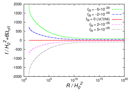
Figure 1: Five different designer $f(R)$ w.r.t. $w_{\textrm{eff}}=-1$ for different initial conditions $f_{Ri}$.

As an example for demonstration, Fig. 1 shows the designer $f(R)$ with respect to $w_{\textrm{eff}}=-1$: five $f(R)$ corresponding to five initial conditions $f_{Ri}$.

We then test these designer models, $f(R;\{w_{0},w_{a},f_{Ri}\})$, via the cosmic-structure observations and the solar-system experiments, as to be shown in the next two subsections.

IV.2 Cosmic-structure test

To test the designer $f(R)$ models via the observations about the cosmic structure formation, for each model we check whether the theoretical prediction of the two ratios, $\Psi/\Phi$ and $G_{\textrm{eff}}/G_{N}$, in Eqs. (21) and (22) can fit the observational constraint in Eqs. (26) and (27) for the present time ($a=1$) and the scale $k=0.01h\mbox{Mpc}^{-1}$, which is the only case (time and scale) we consider in the remaining of the paper. We note that the test of $f(R)$ modified gravity is not sensitive to the choice of the scales.

This observational constraint is deduced from Giannantonio:2009gi where the cosmic expansion history is fitted with the $\Lambda$CDM model. Accordingly, strictly speaking, it can only constrain the designer $f(R)$ with respect to $w_{\textrm{eff}}=-1$. Nevertheless, here we also apply this constraint to other models in order to manifest how various designer $f(R)$ models might be constrained by the current cosmological observations.

IV.2.1 $1\leq\Psi/\Phi<1.996\,$ for $\,\{a=1,k=0.01h\mbox{Mpc}^{-1}\}$

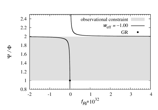
Figure 2: The relation of $\Psi/\Phi$ to $f_{Ri}$ for the $w_{\textrm{eff}}=-1$ designer $f(R)$ model, as presented by the solid curve. The grey region shows the observational constraint of $\Psi/\Phi$, and the dot denotes the GR prediction, $\Psi/\Phi=1$.

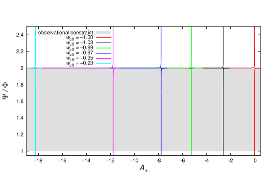
Figure 3: The relation of $\Psi/\Phi$ to $A_{+}$ for the designer $f(R)$ models w.r.t. $w_{\textrm{eff}}=-0.93$, $-0.95$, $-0.97$, $-0.99$, $-1.03$, $-1.00$, as presented by the solid curves from the left to the right, respectively. The constant $A_{+}$ is related to the the initial condition of $f(R)$ through Eqs. (16) and (17). The grey region shows the observational constraint of $\Psi/\Phi$.

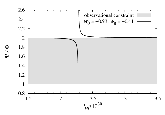
Figure 4: The relation of $\Psi/\Phi$ to $f_{Ri}$ for the designer $f(R)$ models w.r.t. the best fit of the CPL-parametrized $w_{\textrm{eff}}$, i.e., $w_{0}=-0.93$ and $w_{a}=-0.41$. The grey region shows the observational constraint of $\Psi/\Phi$.

For each $w_{\textrm{eff}}$ under consideration we explore numerically the relation of the ratio $\Psi/\Phi(a=1,k=0.01h\mbox{Mpc}^{-1})$ to the initial condition $f_{Ri}$. As an example for demonstration, in Fig. 2 we show the relation of $\Psi/\Phi$ to $f_{Ri}$ for the designer $f(R)$ model with respect to $w_{\textrm{eff}}=-1$, as compared to the observational constraint denoted by the grey region. In addition, we show in Fig. 3 the relation for various constant $w_{\textrm{eff}}$, and in Fig. 4 that for the best fit of the CPL-parametrized $w_{\textrm{eff}}$.

We find this relation similar for different $w_{\textrm{eff}}$: $\Psi/\Phi\cong 2$ for almost all $f_{Ri}$, while it changes violently and goes to $\pm\infty$ within a narrow range of $f_{Ri}$, only in which the designer models may fit the observational constraint in Eq. (26). As a result, one needs to fine-tune the initial condition in order to have a designer $f(R)$ model consistent with the observational results about the cosmic structure formation.

We illustrate the narrow viable range of the initial conditions $f_{Ri}$ in Figs. 5 and 6 for the designer $f(R)$ models with respect to the constant $w_{\textrm{eff}}$ and the CPL-parametrized $w_{\textrm{eff}}$, respectively. We write the viable range as $f_{Ri}=\bar{f}_{Ri}\pm\Delta f_{Ri}$, and present in these plots the central value $\pm\bar{f}_{Ri}$ (denoted by $+$ and $\times$) and the width $2\Delta f_{Ri}$ (denoted by $\ast$) of the viable range.

As have been pointed out above, most of the designer $f(R)$ models predict $\Psi/\Phi\cong 2$, which is around the margin of the current constraint (26). We expect the future cosmological observations will give more detailed and precise information about cosmic structures, and therefore a sharper bound on $\Psi/\Phi$. If the future upper bound of $\Psi/\Phi$ is significantly smaller than $2$, the $f(R)$ modified gravity will be even more fine-tuned and therefore disfavored. On the other hand, if the future observations give a bound excluding unity (the GR prediction), GR will be ruled out.

IV.2.2 $1\leq G_{\textrm{eff}}/G_{N}<1.403\,$ for $\,\{a=1,k=0.01h\mbox{Mpc}^{-1}\}$

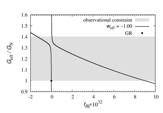
Figure 7: The relation of $G_{\textrm{eff}}/G_{N}$ to $f_{Ri}$ for the $w_{\textrm{eff}}=-1$ designer $f(R)$ model, as presented by the solid curve. The grey region shows the observational constraint of $G_{\textrm{eff}}/G_{N}$, and the dot denotes the GR prediction, $G_{\textrm{eff}}/G_{N}=1$.

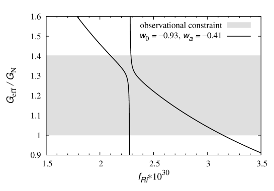
Figure 8: The relation of $G_{\textrm{eff}}/G_{N}$ to $f_{Ri}$ for the designer $f(R)$ models w.r.t. the best fit of the CPL-parametrized $w_{\textrm{eff}}$, i.e., $w_{0}=-0.93$ and $w_{a}=-0.41$. The grey region shows the observational constraint of $G_{\textrm{eff}}/G_{N}$.

For each $w_{\textrm{eff}}$ under consideration we explore numerically the relation of the ratio $G_{\textrm{eff}}/G_{N}(a=1,k=0.01h\mbox{Mpc}^{-1})$ to the initial condition $f_{Ri}$. For demonstration, we show in Fig. 7 the relation for the designer $f(R)$ model with respect to $w_{\textrm{eff}}=-1$, and in Fig. 8 that for the best fit of the CPL-parametrized $w_{\textrm{eff}}$, as compared to the observational constraint denoted by the grey region. We find this relation similar for different $w_{\textrm{eff}}$: $G_{\textrm{eff}}/G_{N}$ smoothly changes with $f_{Ri}$ for most of the initial conditions, but varies violently and goes to $\pm\infty$ within a narrow range of $f_{Ri}$, around which the designer models can fit the observational constraint in Eq. (27). As shown in these two figures, there are two separated viable regions of the initial conditions, one narrow region in the vicinity of the singularity and the other wider region extended to the initial conditions away from the singularity. As a result, the test with the ratio $G_{\textrm{eff}}/G_{N}$ gives a weaker constraint on the designer $f(R)$ models under consideration.

IV.3 Solar-system test

To perform the solar-system test of the designer $f(R)$ models, for each of the models under consideration we check whether the requirement in Eqs. (30) and (31) is satisfied. We examine the designer models constructed with respect to the $w_{\textrm{eff}}$ listed in Sec. IV.1 and a wide range of the initial conditions $f_{Ri}$. As a result, we find the constraint from the solar-system test much more stringent: only the models with $w_{\textrm{eff}}=-1$ and $f_{Ri}\cong 0$, i.e. $f(R)\cong\mbox{constant}$, can fit the constraint. These viable models are very close to the case of GR with a cosmological constant, and therefore cannot be differentiated from the $\Lambda$CDM model, both cosmologically and locally.

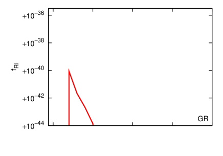
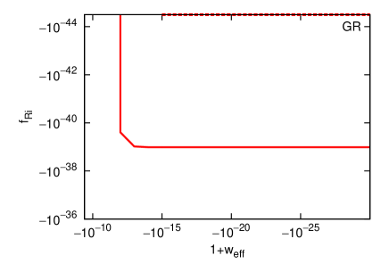
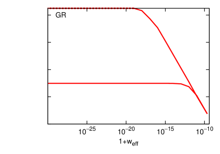
Figure 9: The viable $f(R)$ models in the parameter space $(w_{\textrm{eff}},f_{Ri})$ for constant $w_{\textrm{eff}}$ under the solar-system constraint. The viable region is presented by the red contours in the four plots together. The GR point $(-1,0)$ is between the four plots.

To manifest how close to GR the viable models need to be, we survey in details the small portion of the parameter space $(w_{\textrm{eff}},f_{Ri})$ around the GR point $(-1,0)$ for constant $w_{\textrm{eff}}$. We present the viable region in Fig. 9. This figure shows that even the cases barely different from GR are not viable. Thus, among the designer $f(R)$ models under consideration, only the models closely mimicking GR can pass the solar-system test. Furthermore, we note that the viable models are so close to GR that in these models not only the cosmic expansion is nearly $\Lambda$CDM, but also the key quantities for distinguishing GR from modified gravity in cosmic structures, $\Psi/\Phi$ and $G_{\textrm{eff}}/G_{N}$, agree with the GR prediction (unity) better than $10^{-6}$. Accordingly, these models cannot be differentiated from GR via the cosmological observations, including the observations about the cosmic structure formation and those about the cosmic expansion history. As a result, the solar-system test of gravity rules out the frequently studied $w_{\textrm{eff}}=-1$ designer $f(R)$ models which are cosmologically distinct from $\Lambda$CDM.

V Conclusion and Discussion

In this paper we have investigated three tests of the $f(R)$ theory of modified gravity, including two cosmological tests and one local test. We have invoked the constraints from the observations of (1) the cosmic expansion history and (2) the cosmic structure formation and from (3) the solar-system experiments. We found the constraint from the solar-system test particularly stringent.

To pass the cosmic-expansion test we have considered the designer $f(R)$ models constructed with respect to the constrained effective CPL equation of state $w_{\textrm{eff}}(z)=w_{0}+w_{a}z/(1+z)$ and various initial conditions $f_{Ri}\equiv f_{R}(a=10^{-8})$, and checked whether they pass the other two tests. We have presented the constraint on $f_{Ri}$ from these two tests for each $w_{\textrm{eff}}(z)$. We conclude that the solar-system test rules out all of the designer $f(R)$ models constructed with respect to $w_{\textrm{CPL}}$, except those closely mimicking GR with a cosmological constant, i.e., the $\Lambda$CDM model. In addition, even passing the cosmic-structure test alone would require a fine-tuning of the initial condition of $f(R)$.

We have particularly explored the viable region in the designer-$f(R)$ parameter space $(w_{\textrm{eff}},f_{Ri})$ around the GR point $(-1,0)$ for constant $w_{\textrm{eff}}$, and found it extremely small. Even a tiny deviation from the GR point is ruled out by the solar-system test. The designer models within this viable region are cosmologically indistinguishable from the $\Lambda$CDM model. More precisely, their prediction of the cosmic expansion and the cosmic structure formation agrees with $\Lambda$CDM better than $10^{-6}$. As a result, the frequently studied $w_{\textrm{eff}}=-1$ designer $f(R)$ models that are cosmologically different from $\Lambda$CDM have been ruled out by the solar-system test.

We note that despite the stringent constraint from the solar-system test, it is still possible to construct a viable $f(R)$ model that is observationally different from GR. As pointed out by Gu and Lin in Gu:2010 , the solar-system test gives a severe constraint [Eqs. (30) and (31)] on the behavior of the function $f(R)$ for $R/H_{0}^{2}$ around or larger than $10^{5}$, which corresponds to the time around or before $z\sim 50$. Thus, roughly speaking, the solar-system test and the observations about CMB and BBN require the deviation from GR be extremely small, i.e. $f(R)\cong\mbox{constant}$, from the early time to $z\sim 50$, while a significant deviation from GR is allowed in the present epoch. Accordingly, a viable designer $f(R)$ model can be constructed with respect to the $w_{\textrm{eff}}$ which is close to $-1$ in the past but significantly differs from $-1$ recently. These designer $f(R)$ models are worth consideration in the quest for a modified gravity model that is cosmologically distinct from GR with a cosmological constant.

Figure 5: The viable initial conditions $f_{Ri}=\bar{f}_{Ri}\pm\Delta f_{Ri}$ for the constant-$w_{\textrm{eff}}$ designer $f(R)$ models. The central value $\pm\bar{f}_{Ri}$ is denoted by $+$ or $\times$, and the width $2\Delta f_{Ri}$ of the viable range denoted by $\ast$.

Figure 6: The viable initial conditions $f_{Ri}=\bar{f}_{Ri}\pm\Delta f_{Ri}$ for the CPL-$w_{\textrm{eff}}$ designer $f(R)$ models. The central value $\pm\bar{f}_{Ri}$ is denoted by $+$ or $\times$, and the width $2\Delta f_{Ri}$ of the viable range denoted by $\ast$.

References

- (1) S. Perlmutter et al. [Supernova Cosmology Project Collaboration], Astrophys. J. 517, 565 (1999) [arXiv:astro-ph/9812133].
- (2) A. G. Riess et al. [Supernova Search Team Collaboration], Astron. J. 116, 1009 (1998) [arXiv:astro-ph/9805201].
- (3) D. Huterer and M. S. Turner, Phys. Rev. D 60, 081301 (1999) [arXiv:astro-ph/9808133].
- (4) For a review, see: J. Frieman, M. Turner and D. Huterer, Ann. Rev. Astron. Astrophys. 46, 385 (2008) [arXiv:astro-ph/0803.0982]; E. J. Copeland, M. Sami and S. Tsujikawa, Int. J. Mod. Phys. D 15, 1753 (2006) [arXiv:hep-th/0603057].
- (5) E. Komatsu et al., arXiv:1001.4538 [astro-ph.CO].
- (6) M. Kowalski et al. [Supernova Cosmology Project Collaboration], Astrophys. J. 686, 749 (2008) [arXiv:astro-ph/0804.4142].
- (7) D. J. Eisenstein et al. [SDSS Collaboration], Astrophys. J. 633, 560 (2005) [arXiv:astro-ph/0501171].
- (8) R. Maartens, Living Rev. Rel. 7, 7 (2004) [arXiv:gr-qc/0312059].
- (9) G. R. Dvali, G. Gabadadze and M. Porrati, Phys. Lett. B 485, 208 (2000) [arXiv:hep-th/0005016].
- (10) J. D. Bekenstein, Phys. Rev. D 70, 083509 (2004) [Erratum-ibid. D 71, 069901 (2005)] [arXiv:astro-ph/0403694].
- (11) T. Jacobson and D. Mattingly, Phys. Rev. D 64, 024028 (2001) [arXiv:gr-qc/0007031].
- (12) S. Nojiri and S. D. Odintsov, eConf C0602061, 06 (2006) [Int. J. Geom. Meth. Mod. Phys. 4, 115 (2007)] [arXiv:hep-th/0601213].
- (13) A. A. Starobinsky, Phys. Lett. B 91, 99 (1980).
- (14) S. Capozziello, S. Carloni and A. Troisi, Recent Res. Dev. Astron. Astrophys. 1, 625 (2003) [arXiv:astro-ph/0303041].
- (15) S. M. Carroll, V. Duvvuri, M. Trodden and M. S. Turner, Phys. Rev. D 70, 043528 (2004) [arXiv:astro-ph/0306438].
- (16) T. Chiba, Phys. Lett. B 575, 1 (2003) [arXiv:astro-ph/0307338].
- (17) C. M. Will, Living Rev. Rel. 4, 4 (2001) [arXiv:gr-qc/0103036].
- (18) B. Bertotti, L. Iess and P. Tortora, Nature 425, 374 (2003).
- (19) C. M. Will, Living Rev. Rel. 9, 3 (2005) [arXiv:gr-qc/0510072].
- (20) J. Khoury and A. Weltman, Phys. Rev. Lett. 93, 171104 (2004) [arXiv:astro-ph/0309300].
- (21) J. Khoury and A. Weltman, Phys. Rev. D 69, 044026 (2004) [arXiv:astro-ph/0309411].
- (22) L. Pogosian and A. Silvestri, Phys. Rev. D 77, 023503 (2008) [Erratum-ibid. D 81, 049901 (2010)] [arXiv:astro-ph/0709.0296].
- (23) M. Chevallier and D. Polarski, Int. J. Mod. Phys. D 10, 213 (2001) [arXiv:gr-qc/0009008].
- (24) E. V. Linder, Phys. Rev. Lett. 90, 091301 (2003) [arXiv:astro-ph/0208512].
- (25) T. Faulkner, M. Tegmark, E. F. Bunn and Y. Mao, Phys. Rev. D 76, 063505 (2007) [arXiv:astro-ph/0612569].
- (26) S. Capozziello and S. Tsujikawa, Phys. Rev. D 77, 107501 (2008) [arXiv:gr-qc/0712.2268].
- (27) Y. Bisabr, Phys. Lett. B 683, 96 (2010) [arXiv:0907.3838 [gr-qc]].
- (28) Je-An Gu and Wei-Ting Lin, in preparation (2010).
- (29) S. Tsujikawa, Phys. Rev. D 76, 023514 (2007) [arXiv:0705.1032 [astro-ph]].
- (30) P. Serra, A. Cooray, S. F. Daniel, R. Caldwell and A. Melchiorri, Phys. Rev. D 79, 101301 (2009) [arXiv:0901.0917 [astro-ph.CO]].
- (31) S. F. Daniel et al., Phys. Rev. D 80, 023532 (2009) [arXiv:0901.0919 [astro-ph.CO]].
- (32) J. Guzik, B. Jain and M. Takada, Phys. Rev. D 81, 023503 (2010) [arXiv:0906.2221 [astro-ph.CO]].
- (33) T. Giannantonio, M. Martinelli, A. Silvestri and A. Melchiorri, JCAP 1004, 030 (2010) [arXiv:astro-ph/0909.2045].
- (34) S. F. Daniel, E. V. Linder, T. L. Smith, R. R. Caldwell, A. Cooray, A. Leauthaud and L. Lombriser, Phys. Rev. D 81, 123508 (2010) [arXiv:1002.1962 [astro-ph.CO]].
- (35) R. Bean and M. Tangmatitham, Phys. Rev. D 81, 083534 (2010) [arXiv:1002.4197 [astro-ph.CO]].