The rapid magnetic rotator HR 7355

Abstract

For early type magnetic stars slow, at most moderate rotational velocities have been considered an observational fact. The detection of a multi-kilogauss magnetic field in the B2Vpn star with $P\approx 0.52\,d$ and $v\sin i\approx 300$ km/s has brought down this narrative. We have obtained more than 100 high-resolution, high-S/N echelle spectra in 2009. These spectra provide the most detailed description of the variability of any He-strong star to date. The circumstellar environment is dominated by a rotationally locked magnetosphere out to several stellar radii, causing hydrogen emission. The photosphere is characterized by surface chemical abundance inhomogeneities, with much stronger amplitudes, at least for helium, than slower rotating stars like $\sigma$ Ori E. The highly complex rotational line profile modulations of metal lines are probably a consequence the equatorial gravity darkening of HR 7355, and thus may offer an independent measurement of the von Zeipel parameter $\beta$.

1 Introduction

The Helium-strong star HR 7355 has recently been found to host a strong magnetic field. The short period of $P=0.52$ d puts it among the shortest period non-degenerate magnetic stars known, while its $v\sin i\approx 310$km s ^-1 is the highest for any known non-degenerate magnetic star.

HR 7355 is a star for which effects like gravity darkening and oblate deformation cannot be ignored anymore. This means traditional analysis methods to derive stellar parameters will, at best, give uncertain results, and at worst misleading ones.

The presence of photospheric abundance pattern is intriguing, as in a hot star rotationally induced meridional flows should dilute such pattern quickly. While it has been suggested that the magnetic field would inhibit this circulation, HR 7355 is the first case where this can be tested observationally: not only are there abundance variations across the stellar surface, but the amplitude of the equivalent width of the Hei lines is much larger that in the similar, though less rapidly rotating, Bp star $\sigma$ Ori E.

2 Observations

Apart from archival and literature data this work is based on high-resolution echelle spectra obtained in 2009 with UVES at the 8.2m Kueyen telescope on Cerro Paranal. The instrument was used in its DIC2 437/760 setting, which gives a blue spectrum from about 375 to 498 nm and a red spectrum from about 570 to 950 nm, with a small gap at 760 nm. The slit-width was 0.8 arcsec, giving a resolving power of about $R=50\,000$ over the entire spectrum. The UVES observations were done on three chunks, in April, July, and September 2009.

Exposure times were between 120 seconds in April and 30 seconds July to September, where the shorter exposures were repeated four times. Since the period is short we did not average shorter exposures, but treat them as taken at distinct phases. In total, we have 104 blue and 112 red spectra. The typical $S/N$ of a single spectrum is about 275 in the blue region and 290 in the red.

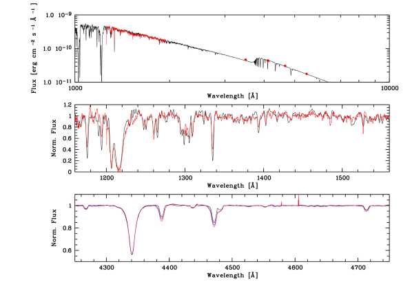
Figure 1: The B3-model vs. observed data: Upper panel: UV IUE short-wavelength spectrophotometry and Strömgren visual photometry vs. modeled fluxes. Middle panel: IUE spectrum vs. modeled UV-line profiles. Lower panel: All UVES (red) and FORS2 (blue) spectra averaged vs. modeled visual line profiles.

3 Stellar parameters

In order to determine the stellar parameters, we made use of spectral synthesis, both for line strength and profiles, as well as for absolute fluxes. The code we used is the third, re-programmed version of Townsend’s ([Townsend (1997), 1997]) BRUCE and KYLIE suite, which in the further we will call “B3”.

In a first step, the profile of Cii 4267, the strongest of all metal lines, was used to obtain the projected rotational velocity of $v\sin i=310\pm 5$ km s^-1, in good agreement with [Oksala et al.(2010), Oksala et al. (2010)]. Together with the rotational period of $P=0.5214404$ d the equatorial radius then becomes $R_{\star,\rm equ.}\sin i=3.19{\rm R_{\odot}}$. Assuming that a rapidly rotating star is constrained by five independent parameters, usually $v_{\rm eq},i,T_{\rm eff},M_{\star},R_{\star}$, this leaves only three of them to be determined, namely the mass, the effective temperature, and the inclination.

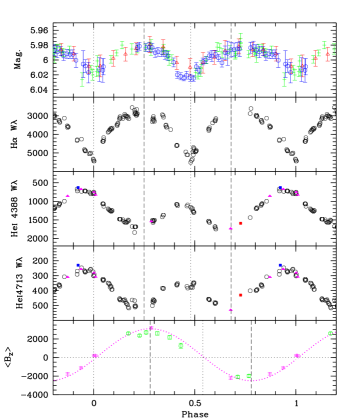
Figure 2: Phased observational data: Photometric data from [Oksala et al.(2010), Oksala et al.(2010)], and ASAS data from [Mikulášek et al.(2010), Mikulášek et al.(2010)] (uppermost), EWs from UVES (middle), with FORS and FEROS $W_{\lambda}$ measurements of Hei 4388, 4713 added, as well as FORS [Rivinius et al.(2010), (Rivinius et al. (2010))] and ESPaDOns magnetic data (lowermost panel).

[Hei] 4045

Hei 4713

Hei 6678

Nei 6717

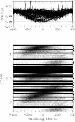
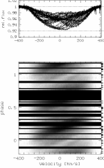
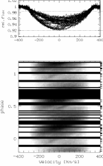
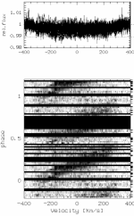
Nii 4631

Cii 4267

Siiii 4553

Sii 4816

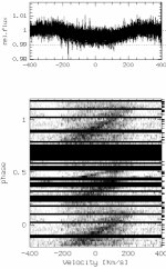
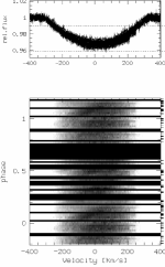
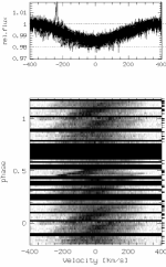
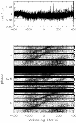
Figure 3: Phased variations of photospheric Helium and metal lines constructed with 64 bins.

The meaning of the effective temperature $T_{\rm eff}$ in a rapidly rotating star is not straightforward, so we note that $T_{\rm eff}$ here is the uniform black-body temperature, that a star of the same surface area would need to have the same full solid angle luminosity as the actual gravity darkened star. The $T_{\rm eff}$ of HR 7355 is constrained using de-reddened flux-calibrated UV spectra (from IUE) and visual photometry. These data are fitted best with $T_{\rm eff}=17\,000$ K (see Fig. 1).

This temperature seems incompatible with the spectral classification of B2. However, due to chemical peculiarity the helium lines are much stronger than they would be for solar abundances, biasing classifications towards the spectral type with the strongest Hei lines, which is B2.

Since $P_{\rm rot}$ and $v\sin i$ are well constrained, the inclination effectively determines the stellar equatorial radius and the geometric projection onto the line of sight, i.e. the area of the star seen. Together with the above derived $T_{\rm eff}$ and the Hipparcos distance, the flux levels of the SED for 17 000 K constrain the inclination, therefore. For $T_{\rm eff}=17\,000$ models with $i=60^{\circ}$ are just so compatible with the flux curve for the closest possible distance; better fitting inclinations result in less plausible parameters elsewhere.

Although this still does not constrain the stellar mass in a straightforward observational way, all the other parameters are sufficiently known to leave only a narrow range of acceptable evolutionary track masses. This is because we can, at least in first order, expect that the luminosity of a star of a given mass does not change with its rotational velocity. The model has a luminosity of about $L_{\star}=1000\,{\rm L_{\odot}}$, and such a luminosity is only compatible with a mass of about $6\pm 0.5$ M_⊙, not with a higher one.

4 Variability

For the ephemeris we adopt the epoch given by [Rivinius et al.(2010), Rivinius et al. (2010)], $T_{0}({\rm MJD})=54\,940.33$, which is the mid-date of an occultation of the star by the magnetospheric material, seen in the Balmer line spectroscopy, and as such very well defined. The best period proved to be the value published by [Oksala et al.(2010), Oksala et al. (2010)], $P=0.5214404$ d, who could rely on a twice as long time-base. Figure 2 shows previously published data together with equivalent width measured in the UVES data, phased with the ephemeris given here.

The H$\alpha$ equivalent widths are fully dominated by variations of the circumstellar environment, there is no indication for a photospherically intrinsic variation of this or any other hydrogen line’s strength. The equivalent width of helium lines like Hei 4713 and 4388 are clearly of a double wave character. Although the strongest EW points in both half-cycles are on a similar level, the weakest EW values differ by a factor of two.

In terms of line profiles, the most obvious photospheric variation is that of the Hei lines. The variations are very strong, in percentage of the line strength much stronger than in other He-strong stars like $\sigma$ Ori E. Figure 2 shows a factor of three to four between the weak and strong states of Hei lines. Other than the figure suggests, however, a detailed look at the spectra shows that the variation is not as plain as consisting of two enhanced polar regions and a depleted belt only, in particular not in the metal lines, which hardly show EW variations, but clear line profile variability (see Fig. 3).

5 Magnetic field and magnetosphere

Constraints on both the inclination $i$ and the obliqueness $\beta$ can be obtained from the observed properties of the magnetic field. Applying standard diagnostics of stellar magnetic fields gives $r=B_{\rm min}/B_{\rm max}=\cos(\beta+i)/\cos(\beta-i)=-0.78$. This means that $\beta+i\lesssim 140^{\circ}$, for which $i=\beta=70^{\circ}$. Since we have determined $i=60^{\circ}$ above, we conclude that both $i$ and $\beta$ are between 60 and 80^∘, in such a way that $\beta+i$ is about 130 to 140^∘. The field strength at the magnetic poles would then be 11 kG. As will be shown in the next paragraph things are probably more complicated than in a pure dipole field, but the above values should at be at least a good approximation.

The measured magnetic curve, when fitted with a sine, has an offset of $+0.3$ kG, magnetic nulls expected to occur at $\phi=0$ and $\phi=0.54$ (dotted lines in lowermost panel of Fig. 2). Yet, the cloud transits are observed to occur at $\phi=0.0$ and $\phi=0.46$ (dotted lines in upper panels of Fig. 2). Similarly, the magnetic poles pointing towards the observer would be expected for $\phi=0.28$ and $0.78$ in case of a sinusoidal variation (dashed lines in lowermost panel of Fig. 2), but spectroscopically, i.e. by maximal He-enhancement, are rather seen at $\phi=0.25$ and $0.68$ (dashed lines in upper panels of Fig. 2). Both these offsets could be explained with a misaligned magnetic dipole wrt. to the stellar center, which would display in a non-sinusoidal variability curve of the magnetic field. Unfortunately, there are not enough magnetic measurements to address this point in detail.

The two occultations occur at phases $\phi=0.0$ and $\phi=0.46$ (Fig. 4). The passing of the lobe is fast, about $\Delta\phi=0.13$ from $-v\sin i$ to $+v\sin i$. If the magnetospheric lobes reached down to the star, this would rather be $\Delta\phi=0.5$. As the crossing time decreases quadratically with distance, there is no absorbing material directly above the star until about 2 R_⋆. A quarter of a cycle later, the emitting material is seen next to the star, and since it is in magnetically bound corotation there is a linear relation between velocity and distance from the stellar surface. The emission has an inner edge at about $600$ km s${}^{-1}\approx 2v\sin i$, which again points to an empty region inside 2 R_⋆. The outer edge of the emission is at a velocity of about $4\times v\sin i$ in H$\alpha$ and $3\times v\sin i$ in Pa₁₄, which gives outer geometrical limits for the lobe emission of about 4 R_⋆ and 3 R_⋆, respectively.

The theoretical line profiles from the B3 modeling are good approximations of the photospheric profile, as seen in Fig. 1. The residuals (Fig. 4) represent the clean circumstellar emission and it is possible to measure Balmer decrements when the emitting material is next to the star. While the values for $D_{54}$ would be in agreement with logarithmic particle densities between 11.7 and 12.5 per cm³, the densities from $D_{34}$ are somewhat higher, at 12.2 to 12.8 per cm³. In any case, these values are close to the optically thick limit, above which the decrements become independent of density.

6 Conclusions

Apart from its high $v\sin i$, HR 7355 is a rather typical member of the class of He-strong stars. Due to its relative proximity and brightness it is an ideal target to study the interplay of rapid rotation effects, like gravity darkening and meridional circulation, with magnetic effects, like chemical peculiarities and inhibition of the meridional circulation and other non-rigid motions. Indeed it seems very unlikely that a relatively strong and ordered field as seen in HR 7355 could give rise to so many distinct zones of Helium and metal abundances.

The presented data, more than 100 high-quality spectra filling the phase diagram, provide an excellent base to apply techniques like Doppler imaging, rigidly rotating magnetosphere models, and Monte-Carlo radiative transfer models.

H$\alpha$

H$\beta$

Pa₁₄

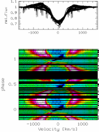
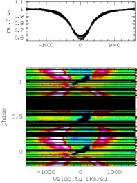
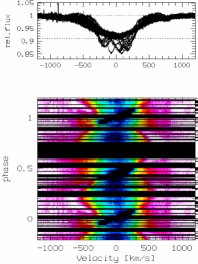
Figure 4: Colour-coded, phased observational variations of the circumstellar magnetosphere. H$\alpha$ and H$\beta$ are the residuals after subtracting the B3 model; the residual level in the line center is unity to better than 1 %. The respective original spectra are overplotted for H$\alpha$ and H$\beta$. Emission clearly seen in residuals, in fact up to H$\delta$. Paschen lines show emission clearly as well, shown here is Pa₁₄; note that these are not residuals and the different abscissa scale. 128 phase bins were used for all panels in order to sample the fast variations around the occultation phases in sufficient detail.

GrohCould you comment on the expected angular extension of the H$\alpha$ and Br$\gamma$ line forming regions and whether those could be resolved by interferometric observations? RiviniusDue to the rigidly rotating magnetosphere, $R_{\rm max}=v_{\rm max}/(v\sin i)$, so for both regions we expect about 3 to 4 stellar radii. For HR 7355 this is well sub-milliarcsecond, but for HR 5907 (see Grunhut et al., this volume) at least the spectrally dispersed phase signature is probably in reach of AMBER/VLTI and the CHARA combiners.

WadeDue to the peculiarities hydrogen may be non-uniformly distributed in the atmosphere. Could the apparent departures from dipolar field topology be due to an effect like this?

RiviniusI would be surprised, since a) already the timing of the magnetosphere occultations, i.e. without looking at the magnetic field at all (except polarity) requires a non-sinusoidal (i.e. non-dipole) field signature and b) also with the ESPaDOnS data, derived from metal and He-lines, a similar argument can be made.

References

- [Mikulášek et al.(2010)] Mikulášek, Z., Krtička, J., Henry, G. W., de Villiers, S. N., Paunzen, E., & Zejda, M. 2010, A&A, 511, L7
- [Oksala et al.(2010)] Oksala, M. E., Wade, G. A., Marcolino, W. L. F., Grunhut, J., Bohlender, D., Manset, N., & Townsend, R. H. D. 2010, MNRAS, 405, L51
- [Rivinius et al.(2010)] Rivinius, T., Szeifert, T., Barrera, L., Townsend, R. H. D., Štefl, S., & Baade, D. 2010, MNRAS, 405, L46
- [Townsend (1997)] Townsend, R. H. D. 1997, MNRAS, 284, 839
- [Townsend (2008)] Townsend, R. H. D. 2008, MNRAS, 389, 559