Analyzing Weighted $\ell_{1}$ Minimization for Sparse Recovery with Nonuniform Sparse Models

Abstract

In this paper we introduce a nonuniform sparsity model and analyze the performance of an optimized weighted $\ell_{1}$ minimization over that sparsity model. In particular, we focus on a model where the entries of the unknown vector fall into two sets, with entries of each set having a specific probability of being nonzero. We propose a weighted $\ell_{1}$ minimization recovery algorithm and analyze its performance using a Grassmann angle approach. We compute explicitly the relationship between the system parameters-the weights, the number of measurements, the size of the two sets, the probabilities of being nonzero- so that when i.i.d. random Gaussian measurement matrices are used, the weighted $\ell_{1}$ minimization recovers a randomly selected signal drawn from the considered sparsity model with overwhelming probability as the problem dimension increases. This allows us to compute the optimal weights. We demonstrate through rigorous analysis and simulations that for the case when the support of the signal can be divided into two different subclasses with unequal sparsity fractions, the optimal weighted $\ell_{1}$ minimization outperforms the regular $\ell_{1}$ minimization substantially. We also generalize the results to an arbitrary number of classes.

1 Introduction

Compressed sensing is an emerging technique of joint sampling and compression that has been recently proposed as an alternative to Nyquist sampling (followed by compression) for scenarios where measurements can be costly [25]. The whole premise is that sparse signals (signals with many zero or negligible elements over a known basis) can be recovered with far fewer measurements than the ambient dimension of the signal itself. In fact, the major breakthrough in this area has been the demonstration that $\ell_{1}$ minimization can efficiently recover a sufficiently sparse vector from a system of underdetermined linear equations [3]. $\ell_{1}$ minimization is usually posed as the convex relaxation of $\ell_{0}$ minimization which solves for the sparsest solution of a system of linear equation and is NP hard.

The conventional approach to compressed sensing assumes no prior information on the unknown signal other than the fact that it is sufficiently sparse over a particular basis. In many applications, however, additional prior information is available. In fact, in many cases the signal recovery problem that compressed sensing addresses is a detection or estimation problem in some statistical setting. Some recent work along these lines can be found in [7], which considers compressed detection and estimation, [8], which studies Bayesian compressed sensing, and [9] which introduces model-based compressed sensing allowing for model-based recovery algorithms. In a more general setting, compressed sensing may be the inner loop of a larger estimation problem that feeds prior information on the sparse signal (e.g., its sparsity pattern) to the compressed sensing algorithm [11, 12].

In this paper we will consider a particular model for the sparse signal where the entries of the unknown vector fall into a number $u$ of classes, with each class having a specific fraction of nonzero entries. The standard compressed sensing model is therefore a special case where there is only one class. As mentioned above, there are many situations where such prior information may be available, such as in natural images, medical imaging, or in DNA microarrays. In the DNA microarrays applications for instance, signals are often block sparse, i.e., the signal is more likely to be nonzero in certain blocks rather than in others [10]. While it is possible (albeit cumbersome) to study this model in full generality, in this paper we will focus on the case where the entries of the unknown signal fall into a fixed number $u$ of categories; in the $i$th set $K_{i}$ with cardinality $n_{i}$, the fraction of nonzero entries is $p_{i}$. This model is rich enough to capture many of the salient features regarding prior information. We refer to the signals generated based on this model as nonuniform sparse signals.

A signal generated based on this model could resemble the vector representation of a natural image in the domain of some linear transform (e.g. Discrete Fourier Transform, Discrete Cosine Transform, Discrete Wavelet Transform, …) or the spatial representation of some biomedical image, e.g., a brain fMRI image. Although a brain fMRI image is not necessarily sparse, the subtraction of the brain image at any moment during an experiment from an initial background image of inactive brain mode is indeed a sparse signal which, demonstrates the additional brain activity during the specific course of experiment. Moreover, depending on the assigned task, the experimenter might have some prior information. For example it might be known that some regions of the brain are more likely to be entangled with the decision making process than the others. This can be captured in the above nonuniform sparse model by considering a higher value $p_{i}$ for the more active region. Similarly, this model is applicable to other problems like network monitoring (see  [18] for an application of compressed sensing and nonlinear estimation in compressed network monitoring), DNA microarrays  [20, 21, 22], astronomy, satellite imaging and many more practical examples.

In this paper we first analyze this model for the case where there are $u\geq 2$ categories of entries, and demonstrate through rigorous analysis and simulations that the recovery performance can be significantly boosted by exploiting the additional information. We find a closed form expression for the recovery threshold for $u=2$. We also generalize the results to the case of $u>2$. A further interesting question to be addressed in future work would be to characterize the gain in recovery percentage as a function of the number of distinguishable classes $u$. It is worth mentioning that a somewhat similar model for prior information has been considered in [6]. There, it has been assumed that part of the support is completely known a priori or due to previous processing. A modification of the regular $\ell_{1}$ minimization based on the given information is proven to achieve significantly better recovery guarantees. As will be discussed, this model can be cast as a special case of the nonuniform sparse model, where the sparsity fraction is equal to unity in one of the classes . Therefore, using the generalized tools of this work, we can explicitly find the recovery thresholds for the method proposed in [6]. This is in contrast to the recovery guarantees of [6] which are given in terms of the restricted isometry property (RIP).

The contributions of the paper are the following. We propose a weighted $\ell_{1}$ minimization approach for sparse recovery where the $\ell_{1}$ norms of different classes ($K_{i}$’s) are assigned different weights $w_{K_{i}}$ ($1\leq i\leq u$). Clearly, one would want to give a larger weight to the entries with a higher chance of being zero and thus further force them to be zero. The second contribution is that we explicitly compute the relationship between $p_{i}$, $w_{K_{i}}$,$\frac{n_{i}}{n}$, $1\leq i\leq u$ and the number of measurements so that the unknown signal can be recovered with overwhelming probability as $n\rightarrow\infty$ (the so-called weak and strong thresholds) for measurement matrices drawn from an i.i.d. Gaussian ensemble. The analysis uses the high-dimensional geometry techniques first introduced by Donoho and Tanner [2, 4] (e.g., Grassmann angles) to obtain sharp thresholds for compressed sensing. However, rather than the neighborliness condition used in [2, 4], we find it more convenient to use the null space characterization of Xu and Hassibi [5, 17]. The resulting Grassmannian manifold approach is a general framework for incorporating additional factors into compressed sensing: in [5] it was used to incorporate approximately sparse signals; here it is used to incorporate prior information and weighted $\ell_{1}$ optimization. Our analytic results allow us to precisely compute the optimal weights for any $p_{i}$,$n_{i}$, $1\leq i\leq u$. We also provide certain robustness conditions for the recovery scheme for compressible signals or under model mismatch. We present simulation results to show the advantages of the weighted method over standard $\ell_{1}$ minimization. Furthermore, the results of this paper for the case of two classes ($u=2$) builds a rigid framework for analyzing certain classes of re-weighted $\ell_{1}$ minimization algorithms. In a re-weighted $\ell_{1}$ minimization algorithm, the post processing information from the estimate of the signal at each step can be viewed as additional prior information about the signal, and can be incorporated into the next step as appropriate weights. In a further work we have been able to analytically prove the threshold improvement in a reweighted $\ell_{1}$ minimization using this framework [19]. It is worth mentioning that we have prepared a software package based on the results of this paper for threshold computation using weighted $\ell_{1}$ minimization, and it is available in [24].

The paper is organized as follows. In the next section we briefly describe the notations that we use throughout the paper. In Section 3 we describe the model and state the principal assumptions of nonuniform sparsity that we are interested in. We also sketch the objectives that we are shooting for and, clarify what we mean by recovery improvement in the weighted $\ell_{1}$ case. In Section 4, we skim through our critical theorems and try to present the big picture of the main results. Section 5 is dedicated to the concrete derivation of these results. In Section 6, we briefly introduce the reweighted $\ell_{1}$ minimization algorithm, and provide some insights in how the derivations of this work can be used to analyze the improved recovery thresholds. In Section 7 some simulation results are presented and are compared to the analytical bounds of the previous sections. The paper ends with a conclusion and discussion of future work in Section 8.

2 Basic Definitions and Notations

Throughout the paper, vectors are denoted by small boldface letters ${\bf x},{\bf w},{\bf z},\cdots$, scalars are shown by small regular letters $a,b,\alpha,\cdots$, and matrices are denoted by bold capital letters(${\bf A},\bf{I},\cdots$). For referring to geometrical objects and subspaces, we use Calligraphic notation, e.g. $\mathcal{Z},{\mathcal{F}},{\mathcal{G}},\mathcal{P},\mathcal{C},\cdots$. This includes the notations that we use to indicate the faces of a high dimensional polytope, or the polytope itself. Sets and random variables are denoted by regular capital letters($K,S,\cdots$). The normal distribution with mean $\mu$ and variance $\sigma^{2}$ is denoted by $\mathcal{N}(\mu,\sigma^{2})$. For functions we use both little and capital letters and it should be generally clear from the context. We use the phrases RHS and LHS as abbreviations for Right Hand Side and Left Hand Side respectively throughout the paper.

Definition 1.

A random variable $Y$ is said to have a Half Normal distribution $HN(0,\sigma^{2})$ if $Y=|X|$ where $X$ is a zero mean normal variable $X\sim\mathcal{N}(0,\sigma^{2})$.

3 Problem Description

We first define the signal model. For completeness, we present a general definition.

Definition 2.

Let $\mathcal{K}=\{K_{1},K_{2},...,K_{u}\}$ be a partition of $\{1,2,\cdots,n\}$, i.e. ($K_{i}\cap K_{j}=\emptyset$ for $i\neq j$, and $\bigcup_{i=1}^{u}K_{i}=\{1,2,...,n\}$), and $P=\{p_{1},p_{2},\cdots,p_{u}\}$ be a set of positive numbers in $[0,1]$. A $n\times 1$ vector ${\bf x}=(x_{1},x_{2},\cdots,x_{n})^{T}$ is said to be a random nonuniformly sparse vector with sparsity fraction $p_{i}$ over the set $K_{i}$ for $1\leq i\leq u$, if ${\bf x}$ is generated from the following random procedure:

• Over each set $K_{i}$, $1\leq i\leq u$, the set of nonzero entries of ${\bf x}$ is a random subset of size $p_{i}|K_{i}|$. In other words, a fraction $p_{i}$ of the entries are nonzero in $K_{i}$. $p_{i}$ is called the sparsity fraction over $K_{i}$. The values of the nonzero entries of ${\bf x}$ can arbitrarily be selected from any symmetric distribution. We can choose $\mathcal{N}(0,1)$ for simplicity.

In Figure 1, a sample nonuniformly sparse signal with Gaussian distribution for nonzero entries is plotted. The number of sets is considered to be $u=2$ and both classes have the same size $\frac{n}{2}$, with $n=1000$. The sparsity fraction for the first class $K_{1}$ is $p_{1}=0.3$, and for the second class $K_{2}$ is $p_{2}=0.05$. In fact, the signal is much sparser in the second half than it is in the first half. The advantageous feature of this model is that all the resulting computations are independent of the actual distribution on the amplitude of the nonzero entries. However, as expected, it is not independent of the properties of the measurement matrix. We assume that the measurement matrix ${\bf A}$ is a $m\times n$ matrix with i.i.d. standard Gaussian distributed $\mathcal{N}(0,1)$ entries, with $\frac{m}{n}=\delta<1$. The measurement vector is denoted by ${\bf y}$ and obeys the following:

$${\bf y}={\bf A}{\bf x}.$$ (1)

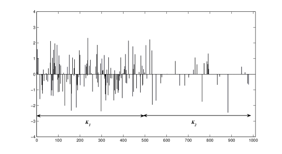
Figure 1: Illustration of a nonuniformly sparse signal.

As mentioned in Section 1, $\ell_{1}$ minimization can recover a randomly selected vector ${\bf x}$ with $k=\mu n$ nonzero entries with high probability, provided $\mu$ is less than a known function of $\delta$. $\ell_{1}$ minimization has the following form:

$$\min_{\bf A{\bf x}={\bf y}}{\|{\bf x}\|_{1}}.$$ (2)

The reference  [2] provides an explicit relationship between $\mu$ and the minimum $\delta$ that guarantees success of $\ell_{1}$ minimization recovery in the case of Gaussian measurements and provides the corresponding numerical curve. The optimization in (2) is a linear program and can be solved polynomially fast ($O(n^{3})$). However, it fails to encapsulate additional prior information of the signal nature, might there be any such information available. One can simply think of modifying (2) to a weighted $\ell_{1}$ minimization as follows:

$$\min_{\bf A{\bf x}={\bf y}}{\|{\bf x}\|_{{\bf w},1}}=\min_{{\bf A}{\bf x}={\bf y}}{\sum_{i=1}^{n}{w_{i}|x_{i}|}}$$ (3)

The index, ${\bf w}$, on the norm is an indication of the $n\times 1$ positive weight vector. Now the questions are i) what is the optimal set of weights for a certain set of available prior information?, and ii) can one improve the recovery threshold using the weighted $\ell_{1}$ minimization of (3) by choosing a set of optimal weights? We have to be more clear with our objective at this point and clarify what we mean by improving the recovery threshold. Generally speaking, if a recovery method can reconstruct all signals of a certain model with certainty, then that method is said to be strongly successful on that signal model. If we have a class of models that can be identified with a parameter $\theta$, and if for all models corresponding to $\theta<\theta_{0}$ a recovery scheme is strongly successful, then the threshold $\theta_{0}$ is called a strong recovery threshold for the parameter $\theta$. For example, for fixed $\frac{m}{n}$, if $k<n$ is sufficiently small, then $\ell_{1}$ minimization can provably recover all $k$-sparse signals, provided that appropriate linear measurements have been made from the signal. The maximum such $k$ is called the strong recovery threshold of the sparsity for the success of $\ell_{1}$ minimization. Likewise, for a fixed ratio $\mu=\frac{k}{n}$, the minimum ratio of measurements to ambient dimension $\frac{m}{n}$ for which, $\ell_{1}$ minimization always recovers $k$-sparse signals from the given $m$ linear measurements is called the strong recovery threshold for the number of measurements for $\ell_{1}$ minimization. In contrast, one can also look into the weak recovery threshold, defined as the threshold below which, with very high probability a random vector generated from the model is recoverable. For the nonuniformly sparse model, the quantity of interest is the overall sparsity fraction of the model defined as ($\frac{\sum_{i=1}^{u}p_{i}n_{i}}{n}$). The question we ask is whether by adjusting $w_{i}$’s according to $p_{i}$’s one can extend the strong or weak recovery threshold for sparsity fraction to a value above the known threshold of $\ell_{1}$ minimization. Equivalently, for given classes $K_{1},\cdots,K_{u}$ and sparsity fractions $p_{i}$’s, how much can the strong or weak threshold be improved for the minimum number of required measurements, as apposed to the case of uniform sparsity with the same overall sparsity fraction.

4 Summary of Main Results

We state the two problems more formally using the notion of recovery thresholds that we defined in the previous section. We only consider the case of $u=2$.

• Problem 1 Consider the random nonuniformly sparse model with two classes $K_{1},K_{2}$ of cardinalities $n_{1}=\gamma_{1}n$ and $n_{2}=\gamma_{2}n$ respectively, and given sparsity fractions $p_{1}$ and $p_{2}$. Let ${\bf w}$ be a given weight vector. As $n\rightarrow\infty$, what is the weak (strong) recovery threshold for $\delta=\frac{m}{n}$ so that a randomly chosen vector (all vectors) ${\bf x}_{0}$ selected from the nonuniformly sparse model is successfully recovered by the weighted $\ell_{1}$ minimization of (3) with high probability?

Upon solving Problem.1, one can exhaustively search for the weight vector ${\bf w}$ that results in the minimum recovery threshold for $\delta$. This is what we recognize as the optimum set of weights. So the second problem can be stated as:

• Problem 2 Consider the random nonuniformly sparse model defined by classes $K_{1},K_{2}$ of cardinalities $n_{1}$ and $n_{2}$ respectively, with $\gamma_{1}=\frac{n_{1}}{n}$ and $\gamma_{2}=\frac{n_{2}}{n}$, and given sparsity fractions $p_{1}$ and $p_{2}$. What is the optimum weight vector ${\bf w}$ in (3) that results in the minimum number of measurements for almost sure recovery of signals generated from the given random nonuniformly sparse model?

We will fully solve these problems in this paper. We first connect the misdetection event to the properties of the measurement matrix. For the non-weighted case, this has been considered in [17] and is known as the null space property. We generalize this result to the case of weighted $\ell_{1}$ minimization, and mention a necessary and sufficient condition for (3) to recover the original signal of interest. The theorem is as follows

Theorem 4.1.

For all $n\times 1$ vectors ${\bf x}^{*}$ supported on the set $K\subseteq\{1,2,...,n\}$, ${\bf x}^{*}$ is the unique solution to the linear program $\min_{{\bf A}{\bf x}={\bf y}}{\sum_{i=1}^{n}{w_{i}|x_{i}|}}$ with ${\bf y}={\bf A}{\bf x}^{*}$, if and only if for every vector ${\bf z}=(z_{1},z_{2},\cdots,z_{n})^{T}$ in the null space of ${\bf A}$, the following holds: $\sum_{i\in K}{w_{i}|z_{i}|}\geq\sum_{i\in\overline{K}}{w_{i}|z_{i}|}$.

This theorem will be proved in Section 5. As will be explained in Section 5.1, Theorem 4.1 along with known facts about the null space of random Gaussian matrices, help us interpret the probability of recovery error in terms of a high dimensional geometrical object called the complementary Grassmann angle; namely the probability that a uniformly chosen $(n-m)$-dimensional subspace $\mathcal{Z}$ shifted by a point ${\bf x}$ of unity weighted $\ell_{1}$-norm, $\sum_{i=1}^{n}w_{i}x_{i}=1$, intersects the weighted $\ell_{1}$-ball $\mathcal{P}_{{\bf w}}=\{{\bf y}\in\mathbb{R}^{n}~{}|\sum_{i=1}^{n}w_{i}|y_{i}|\leq 1\}$ nontrivially at some other point besides ${\bf x}$. The shifted subspace is denoted by ${\mathbf{\mathcal{Z}}}+{\bf x}$. The fact that we can take for granted, without explicitly proving it, is that due to the identical marginal distribution of the entries of ${\bf x}$ in each of the sets $K_{1}$ and $K_{2}$, the entries of the optimal weight vector take at most two (or in the general case $u$) distinct values $w_{K_{1}}$ and $w_{K_{2}}$ depending on their index. In other words

$$\forall i\in\{1,2,\cdots,n\}~{}~{}~{}w_{i}=\left\{\begin{array}[]{c}w_{K_{1}}~{}if~{}i\in K_{1}\\ w_{K_{2}}~{}if~{}i\in K_{2}\end{array}\right.$$ (4)

Leveraging on the existing techniques for computing the complementary Grassmann angle [15, 16], we will be able to state and prove the following theorem along the same lines, which upper bounds the probability that the weighted $\ell_{1}$ minimization does not recover the signal. Please note that in the following theorem, the rigorous mathematical definitions to some of the terms (internal angle and external angle) is not presented, due to the extent of descriptions. They will however be defined rigorously later in the derivations of the main results in Section 5.

Theorem 4.2.

Let $K_{1}$ and $K_{2}$ be two disjoint subsets of $\{1,2,\cdots,n\}$ such that $|K_{1}|=n_{1},|K_{2}|=n_{2}$, and $p_{1}$ and $p_{2}$ be real numbers in $[0,1]$. Also, let $k_{1}=p_{1}n_{1}$, $k_{2}=p_{2}n_{2}$, and $E$ be the event that a random nonuniformly sparse vector ${\bf x}_{0}$ (Definition 2) with sparsity fractions $p_{1}$ and $p_{2}$ over the sets $K_{1}$ and $K_{2}$ respectively is recovered via the weighted $\ell_{1}$ minimization of (3) with ${\bf y}={\bf A}{\bf x}_{0}$. Also, let $E^{c}$ denote the complement event of $E$. Then

$$\mathbb{P}\{E^{c}\} \leq\sum_{{\tiny\begin{array}[]{c}0\leq t_{1}\leq n_{1}-k_{1}\\ 0\leq t_{2}\leq n_{2}-k_{2}\\ t_{1}+t_{2}>m-k_{1}-k_{2}+1\end{array}}}2^{t_{1}+t_{2}+1}{n_{1}-k_{1}\choose t_{1}}{n_{2}-k_{2}\choose t_{2}}\beta(k_{1},k_{2}|t_{1},t_{2})\zeta(t_{1}+k_{1},t_{2}+k_{2})$$ (8)

where $\beta(k_{1},k_{2}|t_{1},t_{2})$ is the internal angle between a $(k_{1}+k_{2}-1)$-dimensional face $\mathcal{F}$ of the weighted $\ell_{1}$-ball $\mathcal{P}_{{\bf w}}=\{y\in\mathbb{R}^{n}|\sum_{i=1}^{n}w_{i}|y_{i}|\leq 1\}$ with $k_{1}$ vertices supported on $K_{1}$ and $k_{2}$ vertices supported on $K_{2}$, and another $(k_{1}+k_{2}+t_{1}+t_{2}-1)$-dimensional face ${\mathcal{G}}$ that encompasses $\mathcal{F}$ and has $t_{1}+k_{1}$ vertices supported on $K_{1}$ and the remaining $t_{2}+k_{2}$ vertices supported on $K_{2}$. $\zeta(d_{1},d_{2})$ is the external angle between a face ${\mathcal{G}}$ supported on set $L$ with $|L\cap K_{1}|=d_{1}$ and $|L\cap K_{2}|=d_{2}$ and the weighted $\ell_{1}$-ball $\mathcal{P}_{{\bf w}}$. See Section 5.1 for the definitions of integral and external angles.

The proof of this theorem will be given in Section 5.2. We are interested in the regimes that make the above upper bound decay to zero as $n\rightarrow\infty$, which requires the cumulative exponent in (8) to be negative. We are able to calculate sharp upper bounds on the exponents of the terms in (8) by using large deviations of sums of normal and half normal variables. More precisely, for small enough $\epsilon$, if we assume that the sum of the terms corresponding to particular indices $t_{1}$ and $t_{2}$ in (8) is denoted by $F(t_{1},t_{2})$, and define $\tau_{1}=\frac{t_{1}}{n}$ and $\tau_{2}=\frac{t_{2}}{n}$, then we are able to find and compute an exponent function $\psi_{tot}(\tau_{1},\tau_{2})=\psi_{com}(\tau_{1},\tau_{2})-\psi_{int}(\tau_{1},\tau_{2})-\psi_{ext}(\tau_{1},\tau_{2})$ so that $\frac{1}{n}\log{F(t_{1},t_{2})}\sim\psi_{tot}(\tau_{1},\tau_{2})$ as $n\rightarrow\infty$. The terms $\psi_{com}(\cdot,\cdot)$, $\psi_{int}(\cdot,\cdot)$ and $\psi_{ext}(\cdot,\cdot)$ are contributions to the cumulative exponent $\psi_{tot}$ by the so called combinatorial, internal angle and external angle terms respectively, existing in the upper bound (8). The derivations of these terms will be elaborated in Section 5.2.3. Consequently, we state a key theorem that is the implicit answer to Problem 1.

Theorem 4.3.

Let $\delta=\frac{m}{n}$ be the ratio of the number of measurements to the signal dimension, $\gamma_{1}=\frac{n_{1}}{n}$ and $\gamma_{2}=\frac{n_{1}}{n}$. For fixed values of $\gamma_{1}$, $\gamma_{2}$, $p_{1}$, $p_{2}$, $\omega=\frac{w_{K_{2}}}{w_{K_{1}}}$ , define $E$ to be the event that a random nonuniformly sparse vector ${\bf x}_{0}$ (Definition 2) with sparsity fractions $p_{1}$ and $p_{2}$ over the sets $K_{1}$ and $K_{2}$ respectively with $|K_{1}|=\gamma_{1}n$ and $|K_{2}|=\gamma_{2}n$ is recovered via the weighted $\ell_{1}$ minimization of (2) with ${\bf y}={\bf A}{\bf x}_{0}$. There exists a critical threshold $\delta_{c}=\delta_{c}(\gamma_{1},\gamma_{2},p_{1},p_{2},\omega)$ such that if $\delta=\frac{m}{n}\geq\delta_{c}$, then $\mathbb{P}\{E^{c}\}$ decays exponentially to zero as $n\rightarrow\infty$. Furthermore, $\delta_{c}$ is given by

$$\boxed{\begin{gathered}\delta_{c}=\min\{\delta~{}|~{}\psi_{com}(\tau_{1},\tau_{2})-\psi_{int}(\tau_{1},\tau_{2})-\psi_{ext}(\tau_{1},\tau_{2})<0~{}\forall~{}0\leq\tau_{1}\leq\gamma_{1}(1-p_{1}),\\ 0\leq\tau_{2}\leq\gamma_{2}(1-p_{2}),\tau_{1}+\tau_{2}>\delta-\gamma_{1}p_{1}-\gamma_{2}p_{2}\}\end{gathered}}$$

where $\psi_{com}$, $\psi_{int}$ and $\psi_{ext}$ are obtained from the following expressions:

Define $g(x)=\frac{2}{\sqrt{\pi}}e^{-{x^{2}}}$, $G(x)=\frac{2}{\sqrt{\pi}}\int_{0}^{x}e^{-y^{2}}dy$ and let $\varphi(.)$ and $\Phi(.)$ be the standard Gaussian pdf and cdf functions respectively.

1. (Combinatorial exponent)

   $$\psi_{com}(\tau_{1},\tau_{2})=\left(\gamma_{1}(1-p_{1})H(\frac{\tau_{1}}{\gamma_{1}(1-p_{1})})+\gamma_{2}(1-p_{2})H(\frac{\tau_{2}}{\gamma_{2}(1-p_{2})})+\tau_{1}+\tau_{2}\right)\log{2}$$ (9)

   where $H(\cdot)$ is the entropy function defined by $H(x)=-x\log{x}-(1-x)\log(1-x)$.

2. (External angle exponent) Define $c=(\tau_{1}+\gamma_{1}p_{1})+\omega^{2}(\tau_{2}+\gamma_{2}p_{2})$, $\alpha_{1}=\gamma_{1}(1-p_{1})-\tau_{1}$ and $\alpha_{2}=\gamma_{2}(1-p_{2})-\tau_{2}$. Let $x_{0}$ be the unique solution to $x$ of the following:

   $$2c-\frac{g(x)\alpha_{1}}{xG(x)}-\frac{\omega g(\omega x)\alpha_{2}}{xG(\omega x)}=0$$

   Then

   $$\psi_{ext}(\tau_{1},\tau_{2})=cx_{0}^{2}-\alpha_{1}\log{G(x_{0})}-\alpha_{2}\log{G(\omega x_{0})}$$ (10)

3. (Internal angle exponent) Let $b=\frac{\tau_{1}+\omega^{2}\tau_{2}}{\tau_{1}+\tau_{2}}$, $\Omega^{\prime}=\gamma_{1}p_{1}+\omega^{2}\gamma_{2}p_{2}$ and $Q(s)=\frac{\tau_{1}\varphi(s)}{(\tau_{1}+\tau_{2})\Phi(s)}+\frac{\omega\tau_{2}\varphi(\omega s)}{(\tau_{1}+\tau_{2})\Phi(\omega s)}$. Define the function $\hat{M}(s)=-\frac{s}{Q(s)}$ and solve for $s$ in $\hat{M}(s)=\frac{\tau_{1}+\tau_{2}}{(\tau_{1}+\tau_{2})b+\Omega^{\prime}}$. Let the unique solution be $s^{*}$ and set $y=s^{*}(b-\frac{1}{\hat{M}(s^{*})})$. Compute the rate function $\Lambda^{*}(y)=sy-\frac{\tau_{1}}{\tau_{1}+\tau_{2}}\Lambda_{1}(s)-\frac{\tau_{2}}{\tau_{1}+\tau_{2}}\Lambda_{1}(\omega s)$ at the point $s=s^{*}$, where $\Lambda_{1}(s)=\frac{s^{2}}{2}+\log(2\Phi(s))$. The internal angle exponent is then given by:

   $$\psi_{int}(\tau_{1},\tau_{2})=(\Lambda^{*}(y)+\frac{\tau_{1}+\tau_{2}}{2\Omega^{\prime}}y^{2}+\log 2)(\tau_{1}+\tau_{2})$$ (11)

Theorem 4.3 is a powerful result, since it allows us to find (numerically) the optimal set of weights for which the fewest possible measurements are needed to recover the signals almost surely. To this end, for fixed values of $\gamma_{1}$, $\gamma_{2}$, $p_{1}$ and $p_{2}$, one should find the ratio $\frac{w_{K_{2}}}{w_{K_{1}}}$ for which the critical threshold $\delta_{c}(\gamma_{1},\gamma_{2},p_{1},p_{2},\frac{w_{K_{2}}}{w_{K_{1}}})$ from Theorem 4.3 is minimum. We discuss this by some examples in Section 7. A generalization of theorem 4.3 for a nonuniform model with an arbitrary number of classes ($u\geq 2$) will be given in Section 5.3.

As mentioned earlier, using Theorem 4.3, it is possible to find the optimal ratio $\frac{w_{K_{2}}}{w_{K_{1}}}$. It however requires an exhaustive search over the $\delta_{c}$ threshold for all possible values of $\omega$. For $\gamma_{1}=\gamma_{2}=0.5$, $p_{1}=0.3$ and $p_{2}=0.05$, we have numerically computed $\delta_{c}(\gamma_{1},\gamma_{2},p_{1},p_{2},\frac{w_{K_{2}}}{w_{K_{1}}})$ as a function of $\frac{w_{K_{2}}}{w_{K_{1}}}$ and depicted the resulting curve in Figure 2a. This suggests that $\frac{w_{K_{2}}}{w_{K_{1}}}\approx 2.5$ is the optimal ratio that one can choose. Later we will confirm this using simulations.

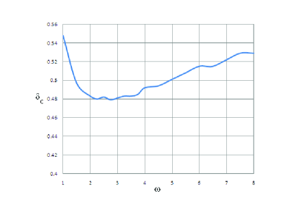
(a) $p_{1}=0.4$, $p_{2}=0.05$.

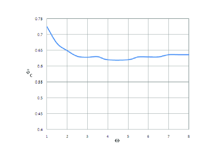
(b) $p_{1}=0.65$, $p_{2}=0.1$.

Figure 2: $\delta_{c}$ as a function of $\omega=\frac{w_{K_{2}}}{w_{K_{1}}}$ for $\gamma_{1}=\gamma_{2}=0.5$.

Note that $\delta_{c}$ given in Theorem 4.3 is a weak bound on the ratio $\delta=\frac{m}{n}$. In other words, it determines the minimum number of measurements so that for a random sparse signal from the nonuniform sparse model and a random support set, the recovery is successful with high probability. It is possible to obtain a strong bound for $\delta$, using a union bound on all possible support sets in the model, and all possible sign patterns of the sparse vector. Similarly, a sectional bound can be defined which accounts for all possible support sets but almost all sign patterns. Therefore, the expressions for the strong and sectional thresholds, which we denote by $\delta_{c}^{(S)}$ and $\delta_{c}^{(T)}$ are very similar to $\delta_{c}$ in Theorem 4.3, except for a slight modification in the combinatorial exponent term $\psi_{com}$. This will be elaborated in Section 5.2.3.

It is worthwhile to consider some asymptotic cases of the presented nonuniform model and some of their implications. First of all, when one of the subclasses is empty, e.g. $\gamma_{1}=0$, then the obtained weak and strong thresholds are equal to the corresponding thresholds of $\ell_{1}$ minimization for a sparsity fraction $p=p_{2}$. Furthermore, if the sparsity fractions $p_{1}$ and $p_{2}$ over the two classes are equal, and a unitary weight $\omega=1$ is used, then the weak threshold $\delta_{c}$ is equal to the threshold of $\ell_{1}$ minimization for a sparsity fraction $p=p_{1}=p_{2}$. In other words:

$$\delta_{c}(\gamma_{1},\gamma_{2},p,p,1)=\delta_{c}(0,1,0,p,1).$$ (12)

This follows immediately from the derivations of the exponents in Theorem 4.3. However, the latter is not necessarily true for the strong threshold. In fact the computation of the strong threshold for regular $\ell_{1}$ minimization involves a union bound over a larger set of possible supports, and therefore the combinatorial exponent becomes larger. Therefore:

$$\delta_{c}^{(S)}(\gamma_{1},\gamma_{2},p,p,1)\leq\delta_{c}^{(S)}(0,1,0,p,1).$$ (13)

A very important asymptotic case is when the unknown signal is fully dense over one of the subclasses, e.g. $p_{1}=1$, which accounts for a partially known support. This model is considered in the work of Vaswani et al. [6], with the motivation that in some applications (or due to previous processing steps), part of the support set can be fully identified. If the dense subclass is $K_{1}$ and $K_{2}=K_{1}^{c}$, then [6] suggests solving the following minimization program:

$$\min_{{\bf A}{\bf x}={\bf y}}\|{\bf x}_{K_{2}}\|_{1}.$$ (14)

It is possible to find exact thresholds for the above problem using the weighted $\ell_{1}$ minimization machinery presented in this paper. First, note that (14) is the asymptotic solution of the following weighted $\ell_{1}$ minimization, when $\omega\rightarrow\infty$

$$\min_{{\bf A}{\bf x}={\bf y}}\|{\bf x}_{K_{1}}\|_{1}+\omega\|{\bf x}_{K_{2}}\|_{1}.$$ (15)

Therefore the recovery threshold for (14) can be given by $\delta_{c}(\gamma_{1},\gamma_{2},1,p_{2},\omega)$ for $\omega\rightarrow\infty$. We prove the following theorem about the latter threshold:

Theorem 4.4.

If $\omega\rightarrow\infty$, then $\delta_{c}(\gamma_{1},\gamma_{2},1,p_{2},\omega)\rightarrow\gamma_{1}+\gamma_{2}\delta_{c}(0,1,0,p_{2},1)$. In other words, when a subset of entries of size $\gamma_{1}n$ are known to be nonzero, the minimum number of measurements that is required for almost surely successful recovery using (14) is equal to the total number of measurements needed if we were allowed to independently make measurements from the two parts and recover each using $\ell_{1}$ minimization.

The proof of this theorem is given in Appendix E.

A very important factor regarding the performance of any recovery method is its robustness. In other words, it is important to understand how resilient the recovery is in the case of compressible signals or in the presence of noise or model mismatch(i.e. incorrect knowledge of the the sets or sparsity factors). We address this in the following theorem.

Theorem 4.5.

Let $K_{1}$ and $K_{2}$ be two disjoint subsets of $\{1,2,\cdots,n\}$, with $|K_{1}|=\gamma_{1}n$,$|K_{2}|=\gamma_{2}n$ and $\gamma_{1}+\gamma_{2}=1$. Also suppose that the dimensions of the measurement matrix ${\bf A}$ satisfy $\delta=\frac{m}{n}\geq\delta_{c}^{(S)}(\gamma_{1},\gamma_{2},p_{1},p_{2},\omega)$ for positive real numbers $p_{1}$ and $p_{2}$ in $[0,1]$ and $\omega>0$. For positive $\epsilon_{1},\epsilon_{2}$, assume that $L_{1}$ and $L_{2}$ are arbitrary subsets of $K_{1}$ and $K_{2}$ with cardinalities $(1-\epsilon_{1})\gamma_{1}p_{1}n$ and $(1-\epsilon_{2})\gamma_{2}p_{2}n$ respectively. With high probability, for every vector ${\bf x}_{0}$, if $\hat{{\bf x}}$ is the solution to the following linear program:

$$\min_{{\bf A}{\bf x}={\bf A}{\bf x}_{0}}\|{\bf x}_{K_{1}}\|_{1}+\omega\|{\bf x}_{K_{2}}\|_{1}.$$ (16)

Then the following holds

$$\|({\bf x}_{0}-\hat{{\bf x}})_{K_{1}}\|_{1}+\omega\|({\bf x}_{0}-\hat{{\bf x}})_{K_{2}}\|_{1}\leq C_{\epsilon_{1},\epsilon_{2}}\left(\|({\bf x}_{0})_{\overline{L_{1}}\cap K_{1}}\|_{1}+\omega\|({\bf x}_{0})_{\overline{L_{2}}\cap K_{2}}\|_{1}\right),$$ (17)

where

$$C_{\epsilon_{1},\epsilon_{2}}=\frac{1+\min(\frac{\epsilon_{1}p_{1}}{1-p_{1}},\frac{\epsilon_{2}p_{2}}{1-p_{2}})}{1-\min(\frac{\epsilon_{1}p_{1}}{1-p_{1}},\frac{\epsilon_{2}p_{2}}{1-p_{2}})}.$$

The above theorem has the following implications. First, if ${\bf x}_{0}$ is a (compressible) vector, such that its “significant” entries follow a nonuniform sparse model, then the recovery error of the corresponding weighted $\ell_{1}$ minimization can be bounded in terms of the $\ell_{1}$ norm of the “insignificant” part of ${\bf x}_{0}$(i.e. the part where a negligible fraction of the energy of the signal is located or most entries have significantly small values, compared to the other part that has an overall large norm). Theorem 4.5 can also be interpreted as the robustness of weighted $\ell_{1}$ scheme to the model mismatch. If $K_{1},K_{2},p_{1},p_{2}$ are the estimates of an actual nonuniform decomposition for ${\bf x}_{0}$ (based on which the minimum number of required measurements have been estimated), then the recovery error can be relatively small if the model estimation error is slight. Theorem 4.5 will be proved in Section 5.4.

5 Derivation of the main results

In this section we provide detailed proofs to the claims of Section 4. Let ${\bf x}_{0}$ be a random nonuniformly sparse signal with sparsity fractions $p_{1}$ and $p_{2}$ over the index subsets $K_{1}$ and $K_{2}$ respectively (Definition 2), and let $|K_{1}|=n_{1}$ and $|K_{2}|=n_{2}$ . Also let $K$ be the support of ${\bf x}$. Let $E$ be the event that ${\bf x}$ is recovered exactly by (3), and $E^{c}$ be its complimentary event. In order to bound the conditional error probability $\mathbb{P}\{E^{c}\}$ we adopt the idea of [17] to interpret the failure recovery event ($E^{c}$) in terms of the null space of the measurement matrix ${\bf A}$. This is stated in Theorem 4.1, which we prove here.

proof of Theorem 4.1.

Suppose the mentioned null space condition holds and define $\hat{{\bf x}}=argmin_{{\bf A}{\bf x}={\bf y}}{\sum_{i=1}^{n}{w_{i}|x_{i}|}}$. Let ${\bf W}=diag(w_{1},w_{2},\cdots,w_{n})$. By triangular inequality, we have:

$$\|{\bf W}\hat{{\bf x}}\|_{1}=\|({\bf W}\hat{{\bf x}})_{K}\|_{1}+\|({\bf W}\hat{{\bf x}})_{\overline{K}}\|_{1} = \|({\bf W}{\bf x}^{*}+{\bf W}\hat{{\bf x}}-{\bf W}{\bf x}^{*})_{K}\|_{1}+\|({\bf W}\hat{{\bf x}})_{\overline{K}}\|_{1}$$

$$\geq \|({\bf W}{\bf x}^{*})_{K}\|_{1}-\|({\bf W}\hat{{\bf x}}-{\bf W}{\bf x}^{*})_{K}\|_{1}+\|({\bf W}\hat{{\bf x}}-{\bf W}{\bf x}^{*})_{\overline{K}}\|_{1}$$

$$\geq \|{\bf W}{\bf x}^{*}\|_{1}$$

Where the last inequality is a result of the fact that $\hat{{\bf x}}-{\bf x}^{*}$ is in the null space of ${\bf A}$ and satisfies the mentioned null space condition. However, by assumption if $\hat{{\bf x}}\neq{\bf x}^{*}$ then $\|{\bf W}\hat{{\bf x}}\|_{1}\leq\|{\bf W}{\bf x}^{*}\|_{1}$. This implies that $\hat{{\bf x}}={\bf x}^{*}$. Conversely, suppose there is some vector ${\bf z}$ in $\mathcal{N}({\bf A})$ such that $\|({\bf W}{\bf z})_{K}\|_{1}>\|({\bf W}{\bf z})_{\overline{K}}\|_{1}$. Taking define ${\bf x}^{*}=({\bf z}_{K}~{}0)^{T}$ and $\hat{{\bf x}}=(0~{}{\bf z}_{\overline{K}})^{T}$ implies that ${\bf A}{\bf x}^{*}={\bf A}\hat{{\bf x}}$ and $\|{\bf W}{\bf x}^{*}\|_{1}>\|{\bf W}\hat{{\bf x}}\|_{1}$. Therefore, ${\bf x}^{*}$ cannot be recovered from the weighted $\ell_{1}$ minimization.   

From this point on, we follow closely the steps towards calculating the upper bound on the failure probability from [5], but with appropriate modifications. The key to our derivations is the following lemma which will be proven in Appendix A.

Lemma 5.1.

For a certain subset $K\subseteq\{1,2,...,n\}$ with $|K|=k$, the event that the null-space $\mathcal{N}(A)$ satisfies

$$\sum_{i\in K}w_{i}|z_{i}|\leq\sum_{i\in\overline{K}}w_{i}|z_{i}|,\forall{\bf z}\in\mathcal{N}(A),$$ (18)

is equivalent to the event that for each ${\bf x}$ supported on the set $K$ (or a subset of $K$)

$$\sum_{i\in K}w_{i}|x_{i}+z_{i}|+\sum_{i\in\overline{K}}w_{i}|z_{i}|\geq\sum_{i\in K}w_{i}|x_{i}|,\forall{\bf z}\in\mathcal{N}(A).$$ (19)

5.1 Upper Bound on the Failure Probability

Knowing Lemma 19, we are now in a position to derive the probability that condition (18) holds for a support set $K$ with $|K|=k$, if we randomly choose an i.i.d. Gaussian matrix ${\bf A}$. In the case of a random i.i.d. Gaussian matrix, the distribution of null space of ${\bf A}$ is right-rotationally invariant, and sampling from this distribution is equivalent to uniformly sampling a random $(n-m)$-dimensional subspace $\mathcal{Z}$ from the Grassmann manifold $\text{Gr}_{(n-m)}(n)$. The Grassmann manifold $\text{Gr}_{(n-m)}(n)$ is defined as the set of all $(n-m)$-dimensional subspaces of $\mathbb{R}^{n}$. We need to upper bound the complementary probability $P=\mathbb{P}\{E^{c}\}$, namely the probability that the (random) support set $K$ of ${\bf x}$ (of random sign pattern) fails the null space condition (19). We denote the null space of ${\bf A}$ by $\mathcal{Z}$. Because $\mathcal{Z}$ is a linear space, for every vector ${\bf z}\in\mathcal{Z}$, $\alpha{\bf z}$ is also in $\mathcal{Z}$ for all $\alpha\in\mathbb{R}$. Therefore, if for a ${\bf z}\in\mathcal{Z}$ and ${\bf x}$ condition (19) fails, by a simple re-scaling of the vectors, we may assume without loss of generality that ${\bf x}$ lies on the surface of any convex ball that surrounds the origin. Therefore we restrict our attention to those vectors ${\bf x}$ from the weighted $\ell_{1}$-sphere:

$$\{{\bf x}\in\mathbb{R}^{n}~{}|~{}\sum_{i=1}^{n}w_{i}|x_{i}|=1\}$$

that are only supported on the set $K$ , or a subset of it. Since we are assuming that the distribution of the nonzero entries of ${\bf x}$ is symmetric, we can write:

$$P=P_{K,-}$$ (20)

where $P_{K,-}$ is the probability that for a specific support set $K$ , there exist a $k$-sparse vector ${\bf x}$ of a specific sign pattern which fails the condition (19). By symmetry, without loss of generality, we assume the signs of the elements of ${\bf x}$ to be non-positive. Now we can focus on deriving the probability $P_{K,-}$. Since ${\bf x}$ is a non-positive $k$-sparse vector supported on the set $K$ and can be restricted to the weighted $\ell_{1}$-sphere $\{{\bf x}\in\mathbb{R}^{n}~{}|~{}\sum_{i=1}^{n}w_{i}|x_{i}|=1\}$, ${\bf x}$ is also on a $(k-1)$-dimensional face, denoted by $\mathcal{F}$, of the weighted $\ell_{1}$-ball $\mathcal{P}_{{\bf w}}$:

$$\mathcal{P}_{{\bf w}}=\{{\bf y}\in\mathbb{R}^{n}~{}|~{}\sum_{i=1}^{n}w_{i}|y_{i}|\leq 1\}$$ (21)

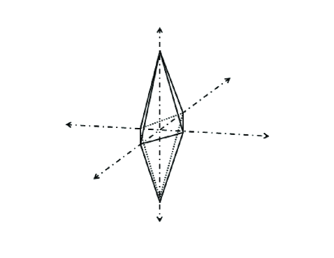
(a)

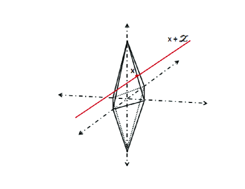
(b)

Figure 3: A weighted $\ell_{1}$-ball, $\mathcal{P}_{{\bf w}}$, in $\mathbb{R}^{3}$ (a), and a linear hyperplane $\mathcal{Z}$ passing through a point ${\bf x}$ in the interior of a one dimensional face of $\mathcal{P}_{{\bf w}}$ (b).

The subscript ${\bf w}$ in $\mathcal{P}_{{\bf w}}$ is an indication of the weight vector ${\bf w}=(w_{1},w_{2},\cdots,w_{n})^{T}$. Figure 3a shows $\mathcal{P}_{{\bf w}}$ in $\mathbb{R}^{3}$ for some nontrivial weight vector ${\bf w}$. Now the probability $P_{K,-}$ is equal to the probability that there exists an ${\bf x}\in{\mathcal{F}}$, and there exists a ${\bf z}\in\mathcal{Z}$ (${\bf z}\neq 0$) such that

$$\sum_{i\in K}w_{i}|x_{i}+z_{i}|+\sum_{i\in\bar{K}}w_{i}|z_{i}|\leq\sum_{i\in K}w_{i}|x_{i}|=1.$$ (22)

We start by studying the case for a specific point ${\bf x}\in{\mathcal{F}}$ and, without loss of generality, we assume ${\bf x}$ is in the relative interior of this $(k-1)$-dimensional face $\mathcal{F}$. For this particular ${\bf x}$ on $\mathcal{F}$, the probability, denoted by $P_{{\bf x}}^{\prime}$, that there exists a ${\bf z}\in\mathcal{Z}$ (${\bf z}\neq 0$) such that

$$\sum_{i\in K}w_{i}|x_{i}+z_{i}|+\sum_{i\in\bar{K}}w_{i}|z_{i}|\leq\sum_{i\in K}w_{i}|x_{i}|=1.$$ (23)

is essentially the probability that a uniformly chosen $(n-m)$-dimensional subspace $\mathcal{Z}$ shifted by the point ${\bf x}$, namely $(\mathcal{Z}+{\bf x})$, intersects the weighted $\ell_{1}$-ball $\mathcal{P}_{{\bf w}}$ non-trivially, namely, at some other point besides ${\bf x}$ (Figure 3b). From the fact that $\mathcal{Z}$ is a linear subspace, the event that $(\mathcal{Z}+{\bf x})$ intersects $\mathcal{P}_{{\bf w}}$ is equivalent to the event that $\mathcal{Z}$ intersects nontrivially with the cone $\mathcal{C}_{{\bf w}}({\bf x})$ obtained by observing the weighted $\ell_{1}$-ball $\mathcal{P}_{{\bf w}}$ from the point ${\bf x}$. (Namely, $\mathcal{C}_{{\bf w}}({\bf x})$ is conic hull of the point set $(\mathcal{P}_{{\bf w}}-{\bf x})$ and of course $\mathcal{C}_{{\bf w}}({\bf x})$ has the origin of the coordinate system as its apex.) However, as noticed in the geometry for convex polytopes [13, 14], the cones $\mathcal{C}_{{\bf w}}({\bf x})$ are identical for any ${\bf x}$ lying in the relative interior of the face $\mathcal{F}$. This means that the probability $P_{K,-}$ is equal to $P_{{\bf x}}^{\prime}$, regardless of the fact that ${\bf x}$ is only a single point in the relative interior of the face $\mathcal{F}$. There are some singularities here because ${\bf x}\in{\mathcal{F}}$ may not be in the relative interior of $\mathcal{F}$, but it turns out that the $\mathcal{C}_{{\bf w}}({\bf x})$ in this case is only a subset of the cone we get when ${\bf x}$ is in the relative interior of $\mathcal{F}$. So we do not lose anything if we restrict ${\bf x}$ to be in the relative interior of the face $\mathcal{F}$, namely we have

$$P_{K,-}=P_{{\bf x}}^{\prime}.$$

Now we only need to determine $P_{{\bf x}}^{\prime}$. From its definition, $P_{{\bf x}}^{\prime}$ is exactly the complementary Grassmann angle [13] for the face $\mathcal{F}$ with respect to the polytope $\mathcal{P}_{{\bf w}}$ under the Grassmann manifold $\text{Gr}_{(n-m)}(n)$: a uniformly distributed $(n-m)$-dimensional subspace $\mathcal{Z}$ from the Grassmannian manifold $\text{Gr}_{(n-m)}(n)$ intersecting non-trivially with the cone $\mathcal{C}_{{\bf w}}({\bf x})$ formed by observing the weighted $\ell_{1}$-ball $\mathcal{P}_{{\bf w}}$ from the relative interior point ${\bf x}\in{\mathcal{F}}$.

Building on the works by L.A. Santalö [15] and P. McMullen [16] in high dimensional geometry and convex polytopes, the complementary Grassmann angle for the $(k-1)$-dimensional face $\mathcal{F}$ can be explicitly expressed as the sum of products of internal angles and external angles [14]:

$$2\times\sum_{s\geq 0}\sum_{G\in\Im_{m+1+2s}(\mathcal{P}_{{\bf w}})}{\beta({\mathcal{F}},{\mathcal{G}})\zeta({\mathcal{G}},\mathcal{P}_{{\bf w}})},$$ (24)

where $s$ is any nonnegative integer, ${\mathcal{G}}$ is any $(m+1+2s)$-dimensional face of the $\mathcal{P}_{{\bf w}}$ ($\Im_{m+1+2s}(\mathcal{P}_{{\bf w}})$ is the set of all such faces), $\beta(\cdot,\cdot)$ stands for the internal angle and $\zeta(\cdot,\cdot)$ stands for the external angle, and are defined as follows [14, 16]:

• An internal angle $\beta({\mathcal{F}}_{1},{\mathcal{F}}_{2})$ is the fraction of the hypersphere $S$ covered by the cone obtained by observing the face $\mathcal{F}_{2}$ from the face $\mathcal{F}_{1}$. The internal angle $\beta({\mathcal{F}}_{1},{\mathcal{F}}_{2})$ is defined to be zero when $\mathcal{F}_{1}\nsubseteq\mathcal{F}_{2}$ and is defined to be one if $\mathcal{F}_{1}={\mathcal{F}}_{2}$.

• An external angle $\zeta(\mathcal{F}_{3},\mathcal{F}_{4})$ is the fraction of the hypersphere $S$ covered by the cone of outward normals to the hyperplanes supporting the face $\mathcal{F}_{4}$ at the face $\mathcal{F}_{3}$. The external angle $\zeta(\mathcal{F}_{3},\mathcal{F}_{4})$ is defined to be zero when $\mathcal{F}_{3}\nsubseteq\mathcal{F}_{4}$ and is defined to be one if $\mathcal{F}_{3}=\mathcal{F}_{4}$.

In order to calculate the internal and external angles, it is important to use the symmetrical properties of the weighted cross-polytope $\mathcal{P}_{{\bf w}}$. First of all, $\mathcal{P}_{{\bf w}}$ is nothing but the convex hull of the following set of $2n$ vertices in $\mathbb{R}^{n}$

$$\mathcal{P}_{{\bf w}}=conv\{\pm\frac{{\bf e}_{i}}{w_{i}}~{}|~{}1\leq i\leq n\}$$ (25)

where ${\bf e}_{i}~{}1\leq i\leq n$ is the standard unit vector in $\mathbb{R}^{n}$ with the $i$th entry equal to $1$. Every $(k-1)$-dimensional face $\mathcal{F}$ of $\mathcal{P}_{{\bf w}}$ is simply the convex hull of $k$ of the linearly independent vertices of $\mathcal{P}_{{\bf w}}$. In that case we say that $\mathcal{F}$ is supported on the index set $K$ of the $k$ indices corresponding to the nonzero coordinates of the vertices of ${\mathcal{F}}$ in $\mathbb{R}^{n}$. More precisely, if $\mathcal{F}=conv\{j_{1}\frac{{\bf e}_{i_{1}}}{w_{i_{1}}},j_{2}\frac{{\bf e}_{i_{2}}}{w_{i_{2}}},\cdots,j_{k}\frac{{\bf e}_{i_{k}}}{w_{i_{k}}}\}$ with $j_{i}\in\{-1,+1\}~{}\forall 1\leq i\leq k$, then ${\mathcal{F}}$ is said to be supported on the set $K=\{i_{1},i_{2},\cdots,i_{k}\}$.

5.2 Special Case of $u=2$

The derivations of the previous section were for a general weight vector ${\bf w}$. We now restrict ourselves to the case of two classes, i.e. $u=2$, namely $K_{1}$ and $K_{2}$ with $|K_{1}|=n_{1}$ and $|K_{2}|=n_{2}$. For this case, we may assume that $w_{i}^{\prime}s$ have the following particular form

$$\forall i\in\{1,2,\cdots,n\}~{}~{}~{}w_{i}=\left\{\begin{array}[]{c}w_{K_{1}}~{}if~{}i\in K_{1}\\ w_{K_{2}}~{}if~{}i\in K_{2}\end{array}\right.$$ (26)

proof of Theorem 4.2.

The choice of ${\bf w}$ as in (26) results in $\mathcal{P}_{{\bf w}}$ having two classes of geometrically identical vertices, and many of faces of $\mathcal{P}_{{\bf w}}$ being isomorphic. In fact, two faces $\mathcal{F}$ and $\mathcal{F}^{\prime}$ of $\mathcal{P}_{{\bf w}}$ that are respectively supported on the sets $K$ and $K^{\prime}$ are geometrically isomorphic if $|K\cap K_{1}|=|K^{\prime}\cap K_{1}|$ and $|K\cap K_{2}|=|K^{\prime}\cap K_{2}|$. In other words the only thing that distinguishes the morphology of the faces of $\mathcal{P}_{{\bf w}}$ is the proportion of their support sets that is located in $K_{1}$ or $K_{2}$. Therefore for two faces ${\mathcal{F}}$ and ${\mathcal{G}}$ with ${\mathcal{F}}$ supported on $K$ and ${\mathcal{G}}$ supported on $L$ ($K\subseteq L$), $\beta(\mathcal{F},\mathcal{G})$ is only a function of the parameters $k_{1}=|K\cap K_{1}|$, $k_{2}=|K\cap K_{2}|$, $k_{1}+t_{1}=|L\cap K_{1}|$ and $k_{2}+t_{1}=|K\cap K_{2}|$. So, instead of $\beta({\mathcal{F}},{\mathcal{G}})$ we may write $\beta(k_{1},k_{2}|t_{1},t_{2})$ to indicate the internal angle internal angle between a $(k_{1}+k_{2}-1)$-dimensional face $\mathcal{F}$ of $\mathcal{P}_{{\bf w}}$ with $k_{1}$ vertices supported on $K_{1}$ and $k_{2}$ vertices supported on $K_{2}$, and a $(k_{1}+k_{2}+t_{1}+t_{2}-1)$-dimensional face ${\mathcal{G}}$ that encompasses $\mathcal{F}$ and has $t_{1}+k_{1}$ vertices supported on $K_{1}$ and the remaining $t_{2}+k_{2}$ vertices supported on $K_{2}$. Similarly instead of $\zeta({\mathcal{G}},\mathcal{P}_{{\bf w}})$ we write $\zeta(t_{1}+k_{1},t_{2}+k_{2})$ to denote the external angle between a face ${\mathcal{G}}$ supported on set $L$ with $|L\cap K_{1}|=d_{1}$ and $|L\cap K_{2}|=d_{2}$, and the weighted $\ell_{1}$-ball $\mathcal{P}_{{\bf w}}$. Using this notation and recalling the formula (24) we can write

$$P_{K,-} = 2\sum_{s\geq 0}\sum_{G\in\Im_{m+1+2s}(\text{SP})}{\beta({\mathcal{F}},{\mathcal{G}})\zeta({\mathcal{G}},\mathcal{P}_{{\bf w}})}$$ (30)

$$= \sum_{{\tiny\begin{array}[]{c}0\leq t_{1}\leq n_{1}-k_{1}\\ 0\leq t_{2}\leq n_{2}-k_{2}\\ t_{1}+t_{2}>m-k_{1}-k_{2}+1\end{array}}}2^{t_{1}+t_{2}+1}{n_{1}-k_{1}\choose t_{1}}{n_{2}-k_{2}\choose t_{2}}\beta(k_{1},k_{2}|t_{1},t_{2})\zeta(t_{1}+k_{1},t_{2}+k_{2}),$$

where in (LABEL:eq:midsumformula) we have used the fact that the number of faces ${\mathcal{G}}$ of $\mathcal{P}_{{\bf w}}$ of dimension $k_{1}+k_{2}+t_{1}+t_{2}-1$ that encompass ${\mathcal{F}}$ and have $k_{1}+t_{1}$ vertices supported on $K_{1}$ and its remaining $k_{2}+t_{2}$ are vertices supported on $K_{2}$ is $2^{t_{1}+t_{2}}{n_{1}-k_{1}\choose t_{1}}{n_{2}-k_{2}\choose t_{2}}$. In fact ${\mathcal{G}}$ has $k_{1}+k_{2}+t_{1}+t_{2}$ vertices including the $k_{1}+k_{2}$ vertices of ${\mathcal{F}}$. The remaining $t_{1}+t_{2}$ vertices can each be independently in the positive or negative orthant, therefore resulting in the term $2^{t_{1}+t_{2}}$. The two other combinatorial terms are the number of ways one can choose $t_{1}$ vertices supported on the set $K_{1}-K$ and $t_{2}$ vertices supported on $K_{2}-K$. From (LABEL:eq:midsumformula) and (20) we can conclude theorem 4.2.   

In the following sub-sections we will derive the internal and external angles for a face ${\mathcal{F}}$, and a face ${\mathcal{G}}$ containing ${\mathcal{F}}$, and will provide closed form upper bounds for them. We combine the terms together and compute the exponents using the Laplace method in Section 5.2.3, and derive thresholds for the negativity of the cumulative exponent.

5.2.1 Computation of Internal Angle

Theorem 5.1.

Let $Z$ be a random variable defined as

$$Z=(k_{1}w_{K_{1}}^{2}+k_{2}w_{K_{2}}^{2})X_{1}-w_{K_{1}}^{2}\sum_{i=1}^{t_{1}}X_{1}^{\prime}-w_{K_{2}}^{2}\sum_{i=1}^{t_{2}}X_{1}^{\prime\prime},$$

where $X_{1}\sim N(0,\frac{1}{2(k_{1}w_{K_{1}}^{2}+k_{2}w_{K_{2}}^{2})})$ is a normal distributed random variable, $X_{i}^{\prime}\sim HN(0,\frac{1}{2w_{K_{1}}^{2}})~{}1\leq i\leq t_{1}$ and $X_{i}^{\prime\prime}\sim HN(0,\frac{1}{2w_{K_{2}}^{2}})~{}1\leq i\leq t_{2}$ are independent (from each other and from $X_{1}$) half normal distributed random variables. Let $p_{Z}(\cdot)$ denote the probability distribution function of $Z$ and $c_{0}=\frac{\sqrt{\pi}}{2^{l-k}}\left((k_{1}+t_{1})w_{K_{1}}^{2}+(k_{2}+t_{2})w_{K_{2}}^{2}\right)^{1/2}$. Then

$$\beta(k_{1},k_{2}|t_{1},t_{2})=c_{0}p_{Z}(0)$$ (32)

We now prove this Theorem. Suppose that ${\mathcal{F}}$ is a $(k-1)$-dimensional face of the weighted $\ell_{1}$-ball

$$\mathcal{P}_{{\bf w}}=\{{\bf y}\in\mathbb{R}^{n}~{}|~{}\sum_{i=1}^{n}w_{i}|y_{i}|\leq 1\}$$

supported on the subset $K$ with $|K|=k=k_{1}+k_{2}$. Let ${\mathcal{G}}$ be a $l-1$ dimensional face of $\mathcal{P}_{{\bf w}}$ supported on the set $L$ with ${\mathcal{F}}\subset{\mathcal{G}}$. Also, let $|L\cap K_{1}|=k_{1}+t_{1}$ and $|L\cap K_{2}|=k_{2}+t_{2}$.

We first state the following lemma the proof of which is given in Appendix B.

Lemma 5.2.

Let ${\mathcal{F}}$ be a $(k-1)$-dimensional face of $\mathcal{P}_{{\bf w}}$ supported on the set $K=\{1,2,\cdots,k\}$, and ${\mathcal{G}}$ be a $l-1$-dimensional face of $\mathcal{P}_{{\bf w}}$ that contains ${\mathcal{F}}$ and is supported on the set $L=\{1,2,\cdots,l\}.$Let $\mathcal{C}_{{\mathcal{F}}^{\perp},{\mathcal{G}}}$ be the positive cone of all the vectors ${\bf x}\in\mathbb{R}^{n}$ that take the form:

$$-\sum_{i=1}^{k}{b_{i}e_{i}}+\sum_{i=k+1}^{l}{b_{i}e_{i}},$$ (33)

where $b_{i},1\leq i\leq l$ are nonnegative real numbers and

$$\sum_{i=1}^{k}{w_{i}b_{i}}=\sum_{i=k+1}^{l}{w_{i}b_{i}},~{}~{}~{}\frac{b_{1}}{w_{1}}=\frac{b_{2}}{w_{2}}=\cdots=\frac{b_{k}}{w_{k}}.$$

Then

$$\int_{\mathcal{C}_{{\mathcal{F}}^{\perp},{\mathcal{G}}}}{e^{-\|{\bf x}\|^{2}}}\,d{\bf x}=\beta({\mathcal{F}},{\mathcal{G}})\cdot\pi^{(l-k)/2}.$$ (34)

From (34) we can find the expression for the internal angle. Define $U\subseteq\mathbb{R}^{l-k+1}$ as the set of all nonnegative vectors $(x_{1},x_{2},\cdots,x_{l-k+1})$ satisfying:

$(\sum_{r=1}^{k}w^{2}_{r})x_{1}=\sum_{r=k+1}^{l}w^{2}_{r}x_{r-k+1}$

and define $f(x_{1},~{}\cdots,~{}x_{l-k+1}):U\rightarrow\mathcal{C}_{F^{\perp},G}$ to be the following linear and bijective map:

$$f(x_{1},\cdots,x_{l-k+1})=-\sum_{r=1}^{k}x_{1}w_{r}{\bf e}_{r}+\sum_{r=k+1}^{l}x_{r-k+1}w_{r}{\bf e}_{r}.$$

Then

$$\int_{\mathcal{C}_{{\mathcal{F}}^{\perp},{\mathcal{G}}}}{e^{-\|{{\bf x}}^{\prime}\|^{2}}}\,d{{\bf x}}^{\prime} =\int_{U}{e^{-\|f({\bf x})\|^{2}}}\,df({\bf x})=|J({\bf M})|\int_{\Gamma}{e^{-\|f(x)\|^{2}}}\,d{x_{2}}\cdots dx_{l-k+1}$$

$$=|J({\bf M})|\int_{\Gamma}e^{-(\sum_{r=1}^{k}{w_{r}^{2}})x_{1}^{2}-\sum_{r=k+1}^{l}{w_{r}^{2}x_{r-k+1}^{2}}}\,d{x_{2}}\cdots dx_{l-k+1}$$ (35)

$\Gamma$ is the region described by

$$(\sum_{r=1}^{k}w^{2}_{r})x_{1}=\sum_{r=k+1}^{l}w^{2}_{r}x_{r-k+1},~{}x_{r}\geq 0~{}~{}2\leq r\leq l-k+1$$ (36)

where $|J({\bf M})|$ is due to the change of integral variables and is essentially the determinant of the Jacobian of the variable transform given by the $l\times(l-k)$ matrix ${\bf M}$ below:

$${\bf M}_{i,j}=\left\{\begin{array}[]{cc}-\frac{1}{\Omega}w_{i}w_{k+j}^{2}&{\scriptsize 1\leq i\leq k,1\leq j\leq l-k}\\ w_{i}&{\scriptsize k+1\leq i\leq l,j=i-k}\\ 0&\text{Otherwise}\end{array}\right.$$ (40)

where $\Omega=\sum_{r=1}^{k}w_{r}^{2}$. The Jacobian is obtained by $|J({\bf M})|=\det({\bf M}^{T}{\bf M})^{1/2}$. By finding the eigenvalues of ${\bf M}^{T}{\bf M}$ we obtain:

$$|J({\bf M})|=w_{K_{1}}^{t_{1}}w_{K_{2}}^{t_{2}}(\frac{\Omega+t_{1}w_{K_{1}}^{2}+t_{2}w_{K_{2}}^{2}}{\Omega})^{1/2}$$ (41)

Now we define a random variable

$$Z=(\sum_{r=1}^{k}w^{2}_{r})X_{1}-\sum_{r=k+1}^{l}w^{2}_{r}X_{r-k+1}$$

where $X_{1},X_{2},\cdots,X_{l-k+1}$ are independent random variables, with $X_{r}\sim HN(0,\frac{1}{2w_{r+k-1}^{2}})$, $2\leq r\leq(l-k+1)$, are half-normal distributed random variables and $X_{1}\sim N(0,\frac{1}{2\sum_{r=1}^{k}{w_{r}^{2}}})$ is a normal distributed random variable. Then by inspection, (35) is equal to $c_{1}p_{Z}(0)$, where $p_{Z}(\cdot)$ is the probability density function for the random variable $Z$ and $p_{Z}(0)$ is the probability density function $p_{Z}(\cdot)$ evaluated at the point $Z=0$, and

$$c_{1} =\frac{\sqrt{\pi}^{l-k+1}}{2^{l-k}}\prod_{q=k+1}^{l}\frac{1}{w_{q}}(\sum_{r=1}^{k}w_{r}^{2})^{1/2}~{}|J(A)|=\frac{\sqrt{\pi}^{l-k+1}}{2^{l-k}}((k_{1}+t_{1})w_{K_{1}}^{2}+(k_{2}+t_{2})w_{K_{2}}^{2})^{1/2}$$ (42)

Combining these results, the proof of Theorem 5.1 is complete.

5.2.2 Computation of External Angle

Theorem 5.2.

The external angle $\zeta({\mathcal{G}},\mathcal{P}_{{\bf w}})=\zeta(d_{1},d_{2})$ between the face ${\mathcal{G}}$ and $\mathcal{P}_{{\bf w}}$ , where $G$ is supported on the set $L$ with $|L\cap K_{1}|=d_{1}$ and $|L\cap K_{2}|=d_{2}$ is given by:

$$\zeta(d_{1},d_{2})=\pi^{-\frac{n-l+1}{2}}2^{n-l}\int_{0}^{\infty}e^{-x^{2}}\left(\int_{0}^{\frac{w_{K_{1}}x}{\xi(d_{1},d_{2})}}e^{-y^{2}}\,dy\right)^{r_{1}}\left(\int_{0}^{\frac{w_{K_{2}}x}{\xi(d_{1},d_{2})}}e^{-y^{2}}\,dy\right)^{r_{2}}\,dx,$$ (43)

Where $\xi^{2}(d_{1},d_{2})=\sum_{i\in L}w_{i}^{2}=d_{1}w_{K_{1}}^{2}+d_{2}w_{K_{2}}^{2}$, $r_{1}=n_{1}-d_{1}$ and $r_{2}=n_{2}-d_{2}$.

Proof.

Without loss of generality, assume that the support set of ${\mathcal{G}}$ is given by $L=\{n-l+1,n-l+2,\cdots,n\}$ and consider the $(l-1)$-dimensional face

$${\mathcal{G}}=\text{conv}\{\frac{{\bf e}_{n-l+1}}{w_{n-l+1}},...,\frac{{\bf e}_{n-k}}{w_{n-k}},\frac{{\bf e}_{n-k+1}}{w_{n-k+1}},...,\frac{{\bf e}_{n}}{w_{n}}\}$$

of the weighted $\ell_{1}$-ball $\mathcal{P}$. The $2^{n-l}$ outward normal vectors of the supporting hyperplanes of the facets containing ${\mathcal{G}}$ are given by

$$\{\sum_{i=1}^{n-l}j_{i}w_{i}{\bf e}_{i}+\sum_{p=n-l+1}^{n}w_{i}{\bf e}_{i},j_{i}\in\{-1,1\}\}.$$

Then the outward normal cone $\mathcal{C}_{{\mathcal{G}},\mathcal{P}_{{\bf w}}}^{\perp}$ at the face ${\mathcal{G}}$ is the positive hull of these normal vectors. Thus

$$\int_{\mathcal{C}_{{\mathcal{G}},\mathcal{P}_{{\bf w}}}^{\perp}}{e^{-\|x\|^{2}}}\,dx =\zeta({\mathcal{G}},\mathcal{P}_{{\bf w}})V_{n-l}(S^{n-l})\int_{0}^{\infty}{e^{-r^{2}}}r^{n-l}\,dx$$

$$=\zeta({\mathcal{G}},\mathcal{P}_{{\bf w}}).\pi^{(n-l+1)/2},$$ (44)

where $V_{n-l}(S^{n-l})$ is the spherical volume of the $(n-l)$-dimensional unit sphere $S^{n-l}$. Now define $U$ to be the set

$$\{x\in R^{n-l+1}\mid x_{n-l+1}\geq 0,|x_{i}/w_{i}|\leq x_{n-l+1},1\leq i\leq(n-l)\}$$

and define $f(x_{1},~{}\cdots,~{}x_{n-l+1}):U\rightarrow\mathcal{C}_{{\mathcal{G}},\mathcal{P}_{{\bf w}}}^{\perp}$ to be the linear and bijective map

$$f(x_{1},~{}\cdots,~{}x_{n-l+1}) = \sum_{i=1}^{n-l}x_{i}{\bf e}_{i}+\sum_{i=n-l+1}^{n}w_{i}x_{n-l+1}{\bf e}_{i}.$$

Then

$$\int_{\mathcal{C}_{{\mathcal{G}},\mathcal{P}_{{\bf w}}}^{\perp}}{e^{-\|x^{\prime}\|^{2}}}\,dx^{\prime}=|J({\bf M})|\int_{U}{e^{-\|f(x)\|^{2}}}\,dx$$

$$=|J({\bf M})|\int_{0}^{\infty}\int_{-w_{K_{1}}x_{n-l+1}}^{w_{K_{1}}x_{n-l+1}}\cdots\int_{-w_{n-l}x_{n-l+1}}^{w_{n-l}x_{n-l+1}}e^{-x_{1}^{2}-\cdots-x_{n-l}^{2}-(\sum_{i=n-l+1}^{n}w_{i}^{2})x_{n-l+1}^{2}}\,dx_{1}\cdots\,dx_{n-l+1}$$

$$=|J({\bf M})|\int_{0}^{\infty}e^{-(\sum_{i=n-l+1}^{n}w_{i}^{2})x^{2}}\left(\int_{-w_{K_{1}}x}^{w_{K_{1}}x}e^{-y^{2}}\,dy\right)^{n_{1}-d_{1}}\left(\int_{-w_{K_{2}}x}^{w_{K_{2}}x}e^{-y^{2}}\,dy\right)^{n_{2}-d_{2}}\,dx$$ (45)

${\bf M}$ is the $n\times(n-l+1)$ change of variable matrix given by ${\bf M}=\left(\begin{array}[]{cc}\bf I_{n-l}&0\\ 0&{\bf w}_{L}\end{array}\right)$, where ${\bf w}_{L}=(w_{n-l+1},w_{n-l+2},\cdots,w_{n})^{T}$. Therefore ${J({\bf M})=\det({\bf M}^{T}{\bf M})}^{1/2}=(d_{1}w_{K_{1}}^{2}+d_{2}w_{K_{2}}^{2})^{1/2}$. Replacing this and a change of variable for $x$ (replace $\xi x$ with $x$) in (45), along with (44), complete the proof.   

5.2.3 Derivation of the Critical Weak and Strong $\delta_{c}$ Threshold

So far we have proved that the probability of the failure event is bounded by the formula

$$\mathbb{P}\{E^{c}\}\leq\sum_{{\tiny\begin{array}[]{c}0\leq t_{1}\leq n_{1}-k_{1}\\ 0\leq t_{2}\leq n_{2}-k_{2}\\ t_{1}+t_{2}>m-k_{1}-k_{2}+1\end{array}}}2^{t_{1}+t_{2}+1}{n_{1}-k_{1}\choose t_{1}}{n_{2}-k_{2}\choose t_{2}}\beta(k_{1},k_{2}|t_{1},t_{2})\zeta(t_{1}+k_{1},t_{2}+k_{2}),$$ (49)

where we gave expressions for $\beta(t_{1},t_{2}|k_{1},k_{2})$ and $\zeta(t_{1}+k_{1},t_{2},k_{2})$ in Sections 5.2.1 and 5.2.2, respectively. Now our objective is to show that the R.H.S of (49) will exponentially decay to $0$ as $n\rightarrow\infty$, provided that $\delta=\frac{m}{n}$ is greater than a critical threshold $\delta_{c}$, which we are trying to evaluate. To do this end we bound the exponents of the combinatorial, internal angle and external angle terms in (49), and find the values of $\delta$ for which the net exponent is strictly negative. The maximum such $\delta$ will give us $\delta_{c}$. Starting with the combinatorial term, we use Stirling approximating on the binomial coefficients to achieve the following as $n\rightarrow\infty$ and $\epsilon\rightarrow 0$

$$\frac{1}{n}\log\left(2^{t_{1}+t_{2}+1}{n_{1}-k_{1}\choose t_{1}}{n_{2}-k_{2}\choose t_{2}}\right)\rightarrow\left(\gamma_{1}(1-p_{1})H(\frac{\tau_{1}}{\gamma_{1}(1-p_{1})})+\gamma_{2}(1-p_{2})H(\frac{\tau_{2}}{\gamma_{2}(1-p_{2})})+\tau_{1}+\tau_{2}\right)\log{2},$$ (50)

where $\tau_{1}=\frac{t_{1}}{n}$ and $\tau_{2}=\frac{t_{2}}{n}$.

For the external angle and internal angle terms we prove the following two exponents

1. Let $g(x)=\frac{2}{\sqrt{\pi}}e^{-{x^{2}}}$, $G(x)=\frac{2}{\sqrt{\pi}}\int_{0}^{x}e^{-y^{2}}dy$. Also define $c=(\tau_{1}+\gamma_{1}p_{1})+\omega^{2}(\tau_{2}+\gamma_{2}p_{2})$, $\alpha_{1}=\gamma_{1}(1-p_{1})-\tau_{1}$ and $\alpha_{2}=\gamma_{2}(1-p_{2})-\tau_{2}$. Let $x_{0}$ be the unique solution to $x$ of the following:

   $$2c-\frac{g(x)\alpha_{1}}{xG(x)}-\frac{\omega g(\omega x)\alpha_{2}}{xG(\omega x)}=0$$

   Define

   $$\psi_{ext}(\tau_{1},\tau_{2})=cx_{0}^{2}-\alpha_{1}\log{G(x_{0})}-\alpha_{2}\log{G(\omega x_{0})}$$ (51)

2. Let $b=\frac{\tau_{1}+\omega^{2}\tau_{2}}{\tau_{1}+\tau_{2}}$ and $\varphi(.)$ and $\Phi(.)$ be the standard Gaussian pdf and cdf functions respectively. Also let $\Omega^{\prime}=\gamma_{1}p_{1}+\omega^{2}\gamma_{2}p_{2}$ and $Q(s)=\frac{\tau_{1}\varphi(s)}{(\tau_{1}+\tau_{2})\Phi(s)}+\frac{\omega\tau_{2}\varphi(\omega s)}{(\tau_{1}+\tau_{2})\Phi(\omega s)}$. Define the function $\hat{M}(s)=-\frac{s}{Q(s)}$ and solve for $s$ in $\hat{M}(s)=\frac{\tau_{1}+\tau_{2}}{(\tau_{1}+\tau_{2})b+\Omega^{\prime}}$. Let the unique solution be $s^{*}$ and set $y=s^{*}(b-\frac{1}{\hat{M}(s^{*})})$. Compute the rate function $\Lambda^{*}(y)=sy-\frac{\tau_{1}}{\tau_{1}+\tau_{2}}\Lambda_{1}(s)-\frac{\tau_{2}}{\tau_{1}+\tau_{2}}\Lambda_{1}(\omega s)$ at the point $s=s^{*}$, where $\Lambda_{1}(s)=\frac{s^{2}}{2}+\log(2\Phi(s))$. The internal angle exponent is then given by:

   $$\psi_{int}(\tau_{1},\tau_{2})=(\Lambda^{*}(y)+\frac{\tau_{1}+\tau_{2}}{2\Omega^{\prime}}y^{2}+\log 2)(\tau_{1}+\tau_{2}).$$ (52)

We now state the following lemmas, which are proved in Appendix C and D.

Lemma 5.3.

Fix $\delta$, $\epsilon>0$. There exists a finite number $n_{0}(\delta,\epsilon)$ such that

$$\frac{1}{n}\log(\zeta(t_{1}+k_{1},t_{2}+k_{2}))<-\psi_{ext}(\tau_{1},\tau_{2})+\epsilon,$$ (53)

uniformly in $0\leq t_{1}\leq n_{1}-k_{1}$, $0\leq t_{2}\leq n_{2}-k_{2}$ and $t_{1}+t_{2}\geq m-k_{1}-k_{2}+1$, $n\geq n_{0}(\delta,\epsilon)$.

Lemma 5.4.

Fix $\delta$, $\epsilon>0$. There exists a finite number $n_{1}(\delta,\epsilon)$ such that

$$\frac{1}{n}\log(\beta(t_{1},t_{2}|k_{1},k_{2}))<-\psi_{int}(\tau_{1},\tau_{2})+\epsilon,$$ (54)

uniformly in $0\leq t_{1}\leq n_{1}-k_{1}$, $0\leq t_{2}\leq n_{2}-k_{2}$ and $t_{1}+t_{2}\geq m-k_{1}-k_{2}+1$, $n\geq n_{1}(\delta,\epsilon)$.

Combining Lemmas 5.3 and 5.4, (50), and the bound in (49) we readily get the critical bound for $\delta_{c}$ as in the Theorem 4.3.

Derivation of the strong and sectional threshold can be easily done using union bounds to account for all possible support sets and/or all sign patterns. The corresponding upper bound on the failure probability for the strong threshold is given by:

$${n_{1}\choose k_{1}}{n_{2}\choose k_{2}}2^{k}P_{K,-}$$ (55)

It then follows that the strong threshold of $\delta$ is given by $\delta_{c}$ in Theorem 4.3, except that the combinatorial exponent $\psi_{com}(\cdot,\cdot)$ must be corrected by adding a term

$$(\gamma_{1}p_{1}+\gamma_{2}p_{2}+\gamma_{1}H(p_{1})+\gamma_{2}H(p_{2}))\log 2,$$ (56)

to the RHS of (9). Similarly, for the sectional threshold, which deals with all possible support sets but almost all sign patterns, the modification in the combinatorial exponent term is as follows:

$$(\gamma_{1}H(p_{1})+\gamma_{2}H(p_{2}))\log 2.$$ (57)

5.3 Generalizations

Except for some subtlety in the large deviation calculations, the generalization of the results of the previous section to an arbitrary $u\geq 2$ classes of entries is straightforward. Consider a nonuniform sparse model with $u$ classes $K_{1},\cdots,K_{u}$ where $|K_{i}|=n_{i}=\gamma_{i}n$, and the sparsity fraction over the set $K_{i}$ is $p_{i}$, and a recovery scheme based on weighted $\ell_{1}$ minimization with weight $\omega_{i}$ for the set $K_{i}$. The bound in (24) is general and can always be used. Due to isomorphism, the internal and external angles $\beta({\mathcal{F}},{\mathcal{G}})$ and $\zeta({\mathcal{G}},\mathcal{P}_{{\bf w}})$ only depend on the number of vertices that the supports of ${\mathcal{F}}$ and ${\mathcal{G}}$ have in common with each $K_{i}$. Therefore, a generalization to (8) would be:

$$\mathbb{P}\{E^{c}\} \leq 2\sum_{{\tiny\begin{array}[]{c}0\leq{\bf t}\leq{\bf n}-{\bf k}\\ \mathbf{1}^{T}{\bf t}>m-\mathbf{1}^{T}{\bf k}+1\end{array}}}\Pi_{1\leq i\leq u}2^{t_{i}}{n_{i}-k_{i}\choose t_{i}}\beta({\bf k}|{\bf t})\zeta({\bf t}+{\bf k})$$ (60)

Where ${\bf t}=(t_{1},\cdots,t_{u})^{T}$, ${\bf k}=(k_{1},\cdots,k_{u})^{T}$ and $\mathbf{1}$ is a vector of all ones. Invoking generalized forms of Theorems 5.2 and 5.1 to approximate the terms $\beta({\bf k}|{\bf t})$ and $\zeta({\bf k}+{\bf t})$, we conclude the following Theorem.

Theorem 5.3.

Consider a nonuniform sparse model with $u$ classes $K_{1},\cdots,K_{u}$ with $|K_{i}|=n_{i}=\gamma_{1}n$, and sparsity fractions $p_{1},p_{2},\cdots,p_{u}$, where $n$ is the signal dimension. Also, let the functions $g(.),G(.),\psi(.),\Psi(.)$ be as defined in Theorem 4.3. For positive values $\{\omega_{i}\}_{i=1}^{u}$, the recovery thresholds (weak,sectional and strong) of the weighted $\ell_{1}$ minimization program:

$$\min_{{\bf A}{\bf x}={\bf y}}\sum_{i=1}^{u}\omega_{i}\|{\bf x}_{K_{i}}\|_{1},$$

is given by the following expression:

$$\boxed{\begin{gathered}\delta_{c}=\min\{\delta~{}|~{}\psi_{com}(\mathbf{\tau})-\psi_{int}(\mathbf{\tau})-\psi_{ext}(\mathbf{\tau})<0~{}\forall\mathbf{\tau}=(\tau_{1},\cdots,\tau_{u})^{T}:\\ ~{}0\leq\tau_{i}\leq\gamma_{i}(1-p_{i})\forall 1\leq i\leq u,\sum_{i=1}^{u}\tau_{i}>\delta-\sum_{i=1}^{u}\gamma_{i}p_{i}\}\end{gathered}}$$

where $\psi_{com}$, $\psi_{int}$ and $\psi_{ext}$ are obtained from the following expressions:

1. $\psi_{com}(\mathbf{\tau})=\log{2}\sum_{i=1}^{u}\gamma_{i}(1-p_{i})H(\frac{\tau_{i}}{\gamma_{i}(1-p_{i})})+\tau_{i},$ for the weak threshold. For sectional threshold this must be modified by adding a term $\log 2\sum_{i=1}^{u}\gamma_{i}H(p_{i})$. For strong threshold, it must be also added with $\sum_{i=1}^{u}\gamma_{i}p_{i}$.

2. $\psi_{ext}(\mathbf{\tau})=cx_{0}^{2}-\sum_{i=1}^{u}\alpha_{i}\log{G(\omega_{i}x_{0})}$, where $c=\sum_{i=1}^{u}\omega_{i}^{2}(\tau_{i}+\gamma_{i}p_{i})$, $\alpha_{i}=\gamma_{i}(1-p_{i})-\tau_{i}$ and $x_{0}$ is the unique solution of $2c=\sum_{i=1}^{u}\omega_{i}\frac{g(\omega_{i}x_{0})\alpha_{i}}{x_{0}G(\omega x_{0})},$

3. $\psi_{int}(\mathbf{\tau})=\lambda(\Lambda^{*}(y)+\frac{\lambda y^{2}}{2\sum_{i=1}^{u}\omega_{i}^{2}\gamma_{i}p_{i}}+\log 2)$, where $\lambda=\sum_{i=1}^{u}\tau_{i}$, and $y$ and $\Lambda^{*}(y)$ are obtained as follows. Let $b=\frac{\sum_{i=1}^{u}\omega_{i}^{2}\tau_{i}}{\lambda}$, $Q(s)=\sum_{i=1}^{u}\frac{\tau_{i}\varphi(s)}{\lambda\Phi(s)}$. Let $s^{*}$ be the solution to $s$ in $-\frac{Q(s)}{s}=b+\frac{\sum_{i=1}^{u}\omega_{i}^{2}\gamma_{i}p_{i}}{\lambda}$, and $y=s^{*}(b-\frac{1}{\hat{M}(s^{*})})$. Then $\Lambda^{*}(y)=s^{*}y-1/\lambda\sum_{i=1}^{u}{\tau_{i}\left(\frac{\omega_{i}^{2}{s^{*}}^{2}}{2}+\log(2\Phi(\omega_{i}s^{*}))\right)}$ .

5.4 Robustness

proof of Theorem 4.5..

We first state the following lemma, which is very similar to Theorem 2 of [5]. We skip its proof for brevity.

Lemma 5.5.

Let $K\subset\{1,2\cdots,n\}$ and the weight vector ${\bf w}=(w_{1},w_{2},\cdots,w_{n})^{T}$ be fixed. Define ${\bf W}=diag(w_{1},w_{2},\cdots,w_{n})$ and suppose $C>1$ is given. For every vector ${\bf x}_{0}\in\mathbb{R}^{n\times 1}$, the solution $\hat{{\bf x}}$ of (3) satisfies

$$\|{\bf W}({\bf x}_{0}-\hat{{\bf x}})\|_{1}\leq 2\frac{C+1}{C-1}\sum_{i\in\overline{K}}w_{i}|(x_{0})_{i}|,$$ (61)

if and only if for every ${\bf z}\in\mathcal{N}({\bf A})$ the following holds:

$$C\sum_{i\in K}w_{i}|z_{i}|\leq\sum_{i\in\overline{K}}w_{i}|z_{i}|.$$ (62)

Let ${\bf z}=(z_{1},\cdots,z_{n})^{T}$ be a vector in the null space of ${\bf A}$, and assume that

$$C^{\prime}\sum_{i\in L_{1}\cup L_{2}}w_{i}|z_{i}|=\sum_{i\in\overline{L_{1}}\cap\overline{L_{2}}}w_{i}|z_{i}|.$$ (63)

Let $K_{\epsilon_{1}}$ and $K_{\epsilon_{2}}$ be the solutions of the following problems

$$K_{\epsilon_{1}} : \max_{K_{\epsilon_{1}}\subset K_{1}\cap\overline{L_{1}},|K_{\epsilon_{1}}|=\epsilon_{1}\gamma_{1}p_{1}n}\sum_{i\in K_{\epsilon_{1}}}w_{i}|z_{i}|,$$ (64)

$$K_{\epsilon_{2}} : \max_{K_{\epsilon_{2}}\subset K_{2}\cap\overline{L_{2}},|K_{\epsilon_{2}}|=\epsilon_{2}\gamma_{2}p_{2}n}\sum_{i\in K_{\epsilon_{2}}}w_{i}|z_{i}|.$$ (65)

Let $L^{\prime}_{1}=L_{1}\cup K_{\epsilon_{1}}$ and $L^{\prime}_{2}=L_{2}\cup K_{\epsilon_{2}}$. From the definition of $K_{\epsilon_{1}}$ and $K_{\epsilon_{2}}$, it follows that

$$\sum_{i\in K_{\epsilon_{1}}}w_{i}|z_{i}| \geq \frac{\epsilon_{1}p_{1}}{1-p_{1}}\sum_{i\in\overline{L^{\prime}_{1}}\cap K_{1}}w_{i}|z_{i}|,$$ (66)

$$\sum_{K_{i\in\epsilon_{2}}}w_{i}|z_{i}| \geq \frac{\epsilon_{2}p_{2}}{1-p_{2}}\sum_{i\in\overline{L^{\prime}_{2}}\cap K_{2}}w_{i}|z_{i}|.$$ (67)

Adding $C^{\prime}\left(\sum_{K_{\epsilon_{1}}}w_{i}|z_{i}|+\sum_{K_{\epsilon_{2}}}w_{i}|z_{i}|\right)$ to both sides of (63) and using (66) and (67), we can write:

$$C^{\prime}\sum_{i\in L^{\prime}_{1}\cup L^{\prime}_{2}}w_{i}|z_{i}| \geq \sum_{i\in\overline{L_{1}}\cap\overline{L_{2}}}w_{i}|z_{i}|+C^{\prime}\left(\frac{\epsilon_{1}p_{1}}{1-p_{1}}\sum_{i\in\overline{L^{\prime}_{1}}\cap K_{1}}w_{i}|z_{i}|+\frac{\epsilon_{2}p_{2}}{1-p_{2}}\sum_{i\in\overline{L^{\prime}_{2}}\cap K_{2}}w_{i}|z_{i}|\right)$$ (68)

$$\geq \left(1+(C^{\prime}+1)\min(\frac{\epsilon_{1}p_{1}}{1-p_{1}},\frac{\epsilon_{2}p_{2}}{1-p_{2}})\right)\sum_{i\in\overline{L^{\prime}_{1}}\cap\overline{L^{\prime}_{2}}}w_{i}|z_{i}|.$$ (69)

Note that $|L^{\prime}_{1}|=\gamma_{1}p_{1}n$ and $|L^{\prime}_{2}|=\gamma_{2}p_{2}n$. Therefore, since $\delta=\frac{m}{n}\geq\delta_{c}^{(S)}(\gamma_{1},\gamma_{2},p_{1},p_{2},\omega)$, we know that $\sum_{i\in L^{\prime}_{1}\cup L^{\prime}_{2}}w_{i}|z_{i}|\leq\sum_{i\in\overline{L^{\prime}_{1}}\cap\overline{L^{\prime}_{2}}}w_{i}|z_{i}|$. From this and (69) we conclude that

$$C^{\prime}\geq\left(1+(C^{\prime}+1)\min(\frac{\epsilon_{1}p_{1}}{1-p_{1}},\frac{\epsilon_{2}p_{2}}{1-p_{2}})\right),$$ (70)

or equivalently

$$C^{\prime}\geq\frac{1+\min(\frac{\epsilon_{1}p_{1}}{1-p_{1}},\frac{\epsilon_{2}p_{2}}{1-p_{2}})}{1-\min(\frac{\epsilon_{1}p_{1}}{1-p_{1}},\frac{\epsilon_{2}p_{2}}{1-p_{2}})}.$$ (71)

Using Lemma 62 and the above inequality, we conclude (17).   

6 Approximate Support Recovery and Reweighted $\ell_{1}$

Using the analytical tools of this paper, it is possible to prove that a class of reweighted $\ell_{1}$ minimization algorithms have a strictly higher recovery thresholds for sparse signals whose nonzero entries follow certain classes of distributions (e.g. Gaussian). The technical details of this claim is not brought here, since it stands beyond the scope of this paper. However, we briefly mention how a simple post processing on the output of $\ell_{1}$ minimization results in a nonuniform sparsity model with $u=2$ classes close to the one we introduced for the unknown signal. A more comprehensive study on this can be found in [12]. The reweighted $\ell_{1}$ recovery algorithm proposed in [12] is composed of two steps. In the first step a standard $\ell_{1}$ minimization is done, and based on the output, a set of entries where the signal is likely to reside (the so-called approximate support) is identified. The unknown signal can thus be thought of as two classes, one with a relatively high fraction of nonzero entries, and one with a small fraction. The second step is a weighted $\ell_{1}$ minimization step where entries outside the approximate support set are penalized with a constant weight larger than $1$. The algorithm is as follows:

Algorithm 1.

1. Solve the $\ell_{1}$ minimization problem:

   $$\hat{{\bf x}}=\arg{\min{\|{\bf z}\|_{1}}}~{}~{}\text{subject to}~{}~{}{\bf A}{\bf z}={\bf A}{\bf x}.$$ (72)

2. Obtain an approximation for the support set of ${\bf x}$: find the index set $L\subset\{1,2,...,n\}$ which corresponds to the largest $k$ elements of $\hat{{\bf x}}$ in magnitude.

3. Solve the following weighted $\ell_{1}$ minimization problem and declare the solution as output:

   $${\bf x}^{*}=\arg{\min\|{\bf z}_{L}\|_{1}+\omega\|{\bf z}_{\overline{L}}\|_{1}}~{}~{}\text{subject to}~{}~{}{\bf A}{\bf z}={\bf A}{\bf x}.$$ (73)

For a given number of measurements, if the support size of ${\bf x}$, namely $k=|K|$, is slightly larger than the sparsity threshold of $\ell_{1}$ minimization, then a so-called robustness of $\ell_{1}$ minimization helps find a lower bound $f_{1}$ for $\frac{|L\cap K|}{|L|}$, i.e. the sparsity fraction of ${\bf x}$ over the set $L$. If $f_{1}$ is sufficiently close to 1, the number of measurements could satisfy:

$$\delta\geq\max_{f^{\prime}_{1}\geq f_{1},f^{\prime}_{1}k+f^{\prime}_{2}(n-k)=k}\delta_{c}^{(T)}(\frac{k}{n},1-\frac{k}{n},f^{\prime}_{1},f^{\prime}_{2},\omega).$$ (74)

Then the recovery is successful in the second step with high probability. Recall that $\delta_{c}^{(T)}$ is the sectional threshold, which accounts for all possible support sets. Therefore, the condition for strict improvement in the reweighted $\ell_{1}$ minimization is that:

$$\delta(0,1,0,\frac{k}{n},1)\geq\max_{f^{\prime}_{1}\geq f_{1},f^{\prime}_{1}k+f^{\prime}_{2}(n-k)=k}\delta_{c}^{(T)}(\frac{k}{n},1-\frac{k}{n},f^{\prime}_{1},f^{\prime}_{2},\omega).$$ (75)

7 Simulation Results

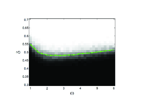
(a) $\gamma_{1}=\gamma_{2}=0.5$, $p_{1}=0.4$ and $p_{2}=0.05$.

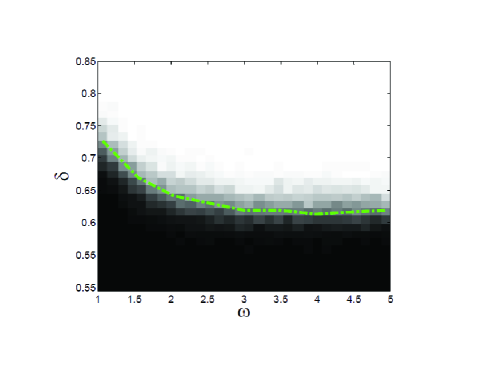
(b) $\gamma_{1}=\gamma_{2}=0.5$, $p_{1}=0.65$ and $p_{2}=0.1$.

Figure 4: Empirical recovery percentage of weighed $\ell_{1}$ minimization for different weight values $\omega$, and different number of measurements $\delta=\frac{m}{n}$ and $n=200$. Signals have been selected from a nonuniform sparse models. White indicates perfect recovery..

We demonstrate by some examples that appropriate weights can boost the recovery percentage. In Figure 4 we have shown the empirical recovery threshold of weighted $\ell_{1}$ minimization for different values of the weight $\omega=\frac{w_{K_{1}}}{w_{K_{2}}}$, for two particular nonuniform sparse models. Note that the empirical threshold is somewhat identifiable with naked eye, and is very similar to the theoretical curve of Figure 2 for similar settings. In another experiment, we fix $p_{2}$ and $n=2m=200$, and try $\ell_{1}$ and weighted $\ell_{1}$ minimization for various values of $p_{1}$. We choose $n_{1}=n_{2}=\frac{n}{2}$. Figure 5a shows one such comparison for $p_{2}=0.05$ and different values of $w_{K_{2}}$. Note that the optimal value of $w_{K_{2}}$ varies as $p_{1}$ changes. Figure 5b illustrates how the optimal weighted $\ell_{1}$ minimization surpasses the ordinary $\ell_{1}$ minimization. The optimal curve is basically achieved by selecting the best weight of Figure 5a for each single value of $p_{1}$. Figure 6 shows the result of simulations in another setting where $p_{2}=0.1$ and $m=0.75n$ (similar to the setting of Section 4). Note that these results very well match the theoretical results of Figures 2a and 2b.

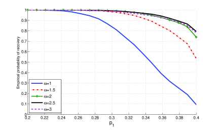
(a)

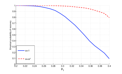
(b)

Figure 5: Empirical probability of successful recovery for weighted $\ell_{1}$ minimization with different weights (unitary weight for the first subclass and $\omega$ for the other one) and suboptimal weights in a nonuniform sparse setting. $p_{2}=0.05$, $\gamma_{1}=\gamma_{2}=0.5$ and $m=0.5n=100$. $\omega^{*}$ is (b) is the optimum value of $\omega$ for each $p_{1}$ among the values shown in (a).

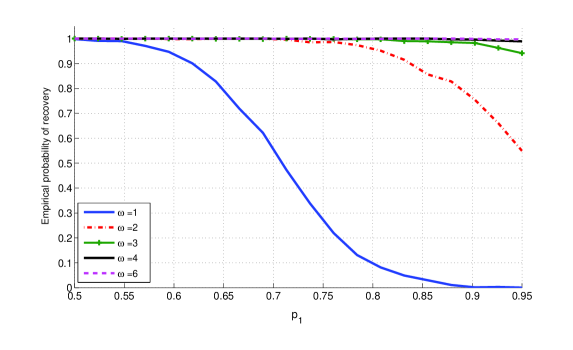
Figure 6: Empirical probability of successful recovery for different weights. $p_{2}=0.1$,$\gamma_{1}=\gamma_{2}=0.5$ and $m=0.75n=150$.

In Figure 7, we have displayed the performance of weighted $\ell_{1}$ minimization in the presence of noise. The original signal is a nonuniformly sparse vector with sparsity fractions $p_{1}=0.4,p_{2}=0.05$ over two subclasses $\gamma_{1}=\gamma_{2}=0.5$. However, a white Gaussian noise vector is added before compression. Figure 7 shows a scatter plot of all output signal to recovery error ratios as a function of the input SNR, for all simulations. In Figure 8 the average curves are compared together for different values of weight $\omega$.

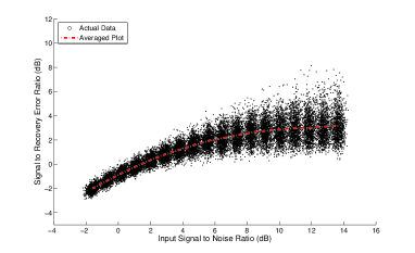
(a) $\omega=1$.

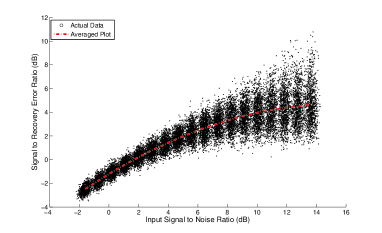
(b) $\omega=3$.

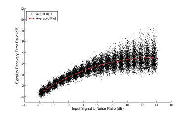
(c) $\omega=5$.

Figure 7: Signal to recovery error ratio for weighted $\ell_{1}$ minimization with weight $\omega$ vs. input SNR for nonuniform sparse signals with $\gamma_{1}=\gamma_{2}=0.5$, $p_{1}=0.4,p_{2}=0.05$ superimposed with Gaussian noise.

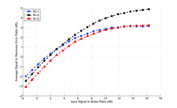
Figure 8: Average signal to recovery error ratio for weighted $\ell_{1}$ minimization with weight $\omega$ vs. input SNR for nonuniform sparse signals with $\gamma_{1}=\gamma_{2}=0.5$, $p_{1}=0.4,p_{2}=0.05$ superimposed with Gaussian noise.

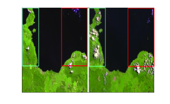
Figure 9: Satellite images taken from the New Britain rainforest in Papua Guina at 1989 (left) and 2000 (right). Image originally belongs to Royal Society for the Protection of Birds and was taken from the Guardian archive, an article on deforestation..

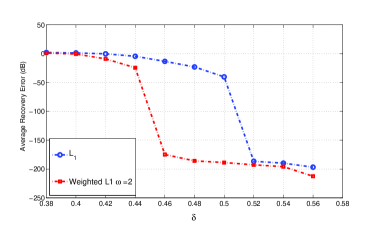
(a)

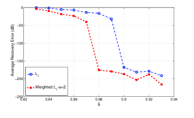
(b)

Figure 10: Average Recovery Error for $\ell_{1}$ and weighted $\ell_{1}$ minimization recovery of the difference between the subframes of a pair of satellite images shown in Figure 9. (a) corresponds to the right(red) subframe in Figure 9, and (b) corresponds to the left(green) frame. Data is averaged over 50 realizations of measurement matrices for each $\delta$.

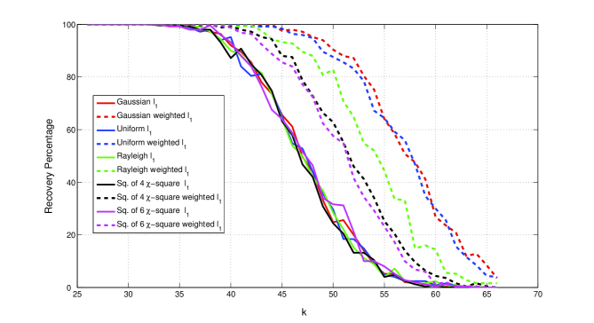
Figure 11: Empirical Recovery Percentage for Algorithm 1 with $n=200$ and $\delta=0.5555$.

We have done some experiments with regular $\ell_{1}$ and weighted $\ell_{1}$ minimization recovery on some real world data. We have chosen a pair of satellite images (Figure 9) taken at two different years, 1989 (left) and 2000 (right), from the New Britain rainforest in Papua Guina. These images are generally recorded to evaluate environmental effects such as deforestation. The difference of images taken at different times is generally not very significant, and thus can be thought of as compressible. In addition, the difference is usually more substantial over certain areas, e.g. forests. Therefore, it can be cast in a nonuniform sparse model. We have applied $\ell_{1}$ minimization to recover the difference image over two subframes, identified by green and red rectangles in Figure 9. In addition, a weighted $\ell_{1}$ minimization is also applied where the frame pixels are divided into two classes of equal sizes, where the concentration of the forestal area is larger over one of the classes, and hence the difference image is less sparse. For the right frame (red), the two classes are bottom half and top half of the frame, and for the left frame (green), they are left half and right half. We casually assign the weight value $\omega=2$ for the sparser region for weighted $\ell_{1}$ recovery, and unitary weight to the denser region. The recovery errors for the two methods are displayed in Figure 10. The error is averaged over $50$ realizations of i.i.d. Gaussian measurement matrix for each $\delta$. As can be seen, even with this value of weight chosen intuitively, the recovery improvement is significant in the weighted $\ell_{1}$ minimization.

In figure 11, we have compared the recovery performance for the regular $\ell_{1}$ minimization and the reweighted $\ell_{1}$ minimization of Algorithm 1, for different sparsity levels and different distributions for the nonzero entries. Here the signal dimension is $n=200$, and the number of measurements is $m=112$, which corresponds to a value of $\delta=0.5555$. We generated random sparse signals with iid entries coming from certain distributions; Gaussian, uniform, Rayleigh , square root of $\chi$-square with 4 degrees of freedom and, square root of $\chi$-square with 6 degrees of freedom. Solid lines represent the simulation results for ordinary $\ell_{1}$ minimization, and different colors indicate different distributions. Dashed lines are used to show the results for Algorithm 1. The reason why these distributions are selected and compared is elaborated in [12], as they demonstrate various levels of improvement. Note that for Gaussian and uniform distributions that are flat and nonzero at the origin, the reweighted algorithm shows an impressive more than 20% improvement in the weak threshold (from 45 to 55).

8 Conclusion and Future Work

We analyzed the performance of the weighted $\ell_{1}$ minimization for nonuniform sparse models. We computed explicitly the phase transition curves for the weighted $\ell_{1}$ minimization, and showed that with proper weighting, the recovery threshold for weighted $\ell_{1}$ minimization can be higher than that of regular $\ell_{1}$ minimization. We provided simulation results to verify this both in the noiseless and noisy situation. Some of our simulations were performed on real world data of satellite images, where the nonuniform sparse model is a valid assumption. A further interesting question to be addressed in future work would be to characterize the gain in recovery percentage as a function of the number of distinguishable classes $u$ in the nonuniform model. In addition, we have used the results of this paper to build iterative reweighted $\ell_{1}$ minimization algorithms that are provably strictly better than $\ell_{1}$ minimization, when the nonzero entries of the sparse signals are known to come from certain distributions (in particular Gaussian distributions) [12, 19]. The basic idea there is that a simple post processing procedure on the output of $\ell_{1}$ minimization results, with high probability, in a hypothetical nonuniform sparsity model for the unknown signal, which can be exploited for improved recovery.

Appendix. Proof of Important Lemmas

Appendix A Proof of Lemma 19

First, let us assume that $\sum_{i\in K}w_{i}|z_{i}|\leq\sum_{i\in\overline{K}}w_{i}|z_{i}|,\forall{\bf z}\in\mathcal{N}(A)$. Note that by assumption $w_{i}$s are all nonnegative. Using the triangular inequality for the weighted $\ell_{1}$ norm (or for each absolute value term on the LHS) we obtain

$$\sum_{i\in K}w_{i}|x_{i}+z_{i}|+\sum_{i\in\overline{K}}w_{i}|z_{i}| \geq \sum_{i\in K}w_{i}|x_{i}|-\sum_{i\in K}w_{i}|z_{i}|+\sum_{i\in\overline{K}}w_{i}|z_{i}|$$

$$\geq \sum_{i\in K}w_{i}|x_{i}|.$$

thus proving the forward part of this lemma. Now let us assume instead that $\exists{\bf z}\in\mathcal{N}(A)$, such that $\sum_{i\in K}w_{i}|z_{i}|>\sum_{i\in\overline{K}}w_{i}|z_{i}|$. Then we can construct a vector ${\bf x}$ supported on the set $K$ (or a subset of $K$), with ${\bf x}_{K}=-{\bf z}_{K}$ (i.e. $x_{i}=-z_{i}~{}\forall i\in K$). Then we have

$$\sum_{i\in K}w_{i}|x_{i}+z_{i}|+\sum_{i\in\overline{K}}w_{i}|z_{i}|=0+\sum_{i\in\overline{K}}w_{i}|z_{i}|<\sum_{i\in K}w_{i}|x_{i}|$$

proving the reverse part of this lemma.

Appendix B Proof of Lemma 5.2

Without loss of generality, assume that ${\mathcal{F}}$ has the following $k$ vertices: $\{\frac{{\bf e}_{r}}{w_{r}},1\leq r\leq k\}$, where ${\bf e}_{r}$ is the $n$-dimensional standard unit vector with the $r$-th element equal to 1. Also assume that the $(l-1)$-dimensional face $G$ is the convex hull of the following $l$ vertices: $\frac{{\bf e}_{r}}{w_{r}},1\leq r\leq l$. Then the cone $\mathcal{C}_{{\mathcal{F}},{\mathcal{G}}}$ formed by observing the $(l-1)$-dimensional face ${\mathcal{G}}$ of the weighted $\ell_{1}$-ball $\mathcal{P}_{{\bf w}}$ from an interior point $x^{{\mathcal{F}}}$ of the face ${\mathcal{F}}$ is the positive cone of the vectors:

$$\frac{{\bf e}_{j}}{w_{j}}-\frac{{\bf e}_{i}}{w_{i}},~{}~{}\text{for all}~{}~{}j\in{J\backslash K},~{}i\in{K},$$ (76)

and also the vectors

$$\frac{{\bf e}_{i_{1}}}{w_{i_{1}}}-\frac{{\bf e}_{i_{2}}}{w_{i_{2}}},~{}~{}\text{for all}~{}~{}{i_{1}}\in{K},~{}{i_{2}}\in{K},$$ (77)

where $L=\{1,2,...,l\}$ is the support set for the face ${\mathcal{G}}$. So the cone $\mathcal{C}_{{\mathcal{F}},{\mathcal{G}}}$ is the direct sum of the linear hull $\mathcal{L}_{{\mathcal{F}}}=\text{lin}\{{\mathcal{F}}-x^{{\mathcal{F}}}\}$ formed by the vectors in (77) and the cone $\mathcal{C}_{{\mathcal{F}}^{\perp},G}=\mathcal{C}_{F,G}\bigcap\mathcal{\mathcal{L}}_{{\mathcal{F}}}^{\perp}$, where $\mathcal{L}_{F}^{\perp}$ is the orthogonal complement to the linear subspace $\mathcal{L}_{{\mathcal{F}}}$. Then $\mathcal{C}_{{\mathcal{F}}^{\perp},{\mathcal{G}}}$ has the same (relative) spherical volume as $\mathcal{C}_{{\mathcal{F}},{\mathcal{G}}}$, and by definition the internal angle $\beta({\mathcal{F}},{\mathcal{G}})$ is the relative spherical volume of the cone $\mathcal{C}_{{\mathcal{F}},{\mathcal{G}}}$. Now let us analyze the structure of $\mathcal{C}_{{\mathcal{F}}^{\perp},{\mathcal{G}}}$. We notice that the vector ${\bf e}_{0}=\sum_{r=1}^{k}w_{r}{\bf e}_{r}$ is in the linear space $\mathcal{L}_{{\mathcal{F}}}^{\perp}$ and is also the only such a vector (up to linear scaling) supported on $K$. Thus a vector ${\bf x}$ in the positive cone $\mathcal{C}_{{\mathcal{F}}^{\perp},{\mathcal{G}}}$ must take the form

$$-\sum_{i=1}^{k}{b_{i}e_{i}}+\sum_{i=k+1}^{l}{b_{i}e_{i}},$$ (78)

where $b_{i},1\leq i\leq l$ are nonnegative real numbers and

$$\sum_{i=1}^{k}{w_{i}b_{i}}=\sum_{i=k+1}^{l}{w_{i}b_{i}}~{}~{}~{}\frac{b_{1}}{w_{K_{1}}}=\frac{b_{2}}{w_{K_{2}}}=\cdots=\frac{b_{k}}{w_{k}}.$$

Now that we have identified $\mathcal{C}_{{\mathcal{F}}^{\perp},{\mathcal{G}}}$ we try to calculate its relative spherical volume with respect to the sphere surface $S^{l-k-1}$ to derive $\beta({\mathcal{F}},{\mathcal{G}})$. First, we notice that $\mathcal{C}_{{\mathcal{F}}^{\perp},{\mathcal{G}}}$ is a $(l-k)$-dimensional cone. Also, all the vectors $(x_{1},\cdots,x_{n})$ in the cone $\mathcal{C}_{{\mathcal{F}}^{\perp},{\mathcal{G}}}$ take the form in (78). From [23],

$$\int_{\mathcal{C}_{{\mathcal{F}}^{\perp},{\mathcal{G}}}}{e^{-\|{\bf x}\|^{2}}}\,d{\bf x}=\beta({\mathcal{F}},{\mathcal{G}})V_{l-k-1}(S^{l-k-1})\int_{0}^{\infty}{e^{-r^{2}}}r^{l-k-1}\,dx=\beta({\mathcal{F}},{\mathcal{G}})\cdot\pi^{(l-k)/2},$$

where $V_{l-k-1}(S^{l-k-1})$ is the spherical volume of the $(l-k-1)$-dimensional sphere $S^{l-k-1}$ and is given by the well-known formula

$$V_{i-1}(S^{i-1})=\frac{i\pi^{\frac{i}{2}}}{\Gamma(\frac{i}{2}+1)},$$

where $\Gamma(\cdot)$ is the usual Gamma function. This completes the proof.

Appendix C Proof of Lemma 5.3

Let $G$ denote the cumulative distribution function of a half-normal $HN(0,1/2)$ random variable, i.e. a random variable $X=|Z|$ where $Z\sim N(0,1/2)$, and $G(x)=\mathbb{P}\{X\leq x\}$. Since $X$ has density function $g(x)=\frac{2}{\sqrt{\pi}}\exp(-x^{2})$, we know that

$$G(x)=\frac{2}{\sqrt{\pi}}\int_{0}^{x}e^{-y^{2}}\,dy;$$ (79)

and so $G$ is just the classical error function erf($\cdot$). We now justify the external angle exponent computations in Theorem 4.3 and Lemma 5.3 using Laplace methods [4]. Using the same set of notations as in Theorem 4.3, let $t_{1}=\tau_{1}n$, $t_{2}=\tau_{2}n$. Also define $c=(\tau_{1}+\gamma_{1}p_{1})+\omega^{2}(\tau_{2}+\gamma_{2}p_{2})$, $\alpha_{1}=\gamma_{1}(1-p_{1})-\tau_{1}$ and $\alpha_{2}=\gamma_{2}(1-p_{2})-\tau_{2}$. Let $x_{0}$ be the unique solution to $x$ of the following:

$$2c-\frac{g(x)\alpha_{1}}{xG(x)}-\frac{\omega g(\omega x)\alpha_{2}}{xG(\omega x)}=0$$ (80)

Since $xG(x)$ is a smooth strictly increasing function ( $\sim 0$ as $x\rightarrow 0$ and $\sim x$ as $x\rightarrow\infty$), and $g(x)$ is strictly decreasing, the function $\frac{g(x)\alpha_{1}}{xG(x)}+\frac{\omega g(\omega x)\alpha_{2}}{xG(\omega x)}$ is one-one on the positive axis, and $x_{0}$ is a well-defined function of $\tau_{1}$ and $\tau_{2}$. Hence, we denote it as $x_{0}(\tau_{1},\tau_{2})$. Then

$$\psi_{ext}(\tau_{1},\tau_{2})=cx_{0}^{2}-\alpha_{1}\log{G(x_{0})}-\alpha_{2}\log{G(\omega x_{0})}.$$ (81)

To prove Lemma 5.3, we start from the explicit integral formula

$$\zeta(d_{1},d_{2})=\pi^{-\frac{n-l+1}{2}}2^{n-l}\int_{0}^{\infty}e^{-x^{2}}\left(\int_{0}^{\frac{w_{K_{1}}x}{\xi(d_{1},d_{2})}}e^{-y^{2}}\,dy\right)^{r_{1}}\left(\int_{0}^{\frac{w_{K_{2}}x}{\xi(d_{1},d_{2})}}e^{-y^{2}}\,dy\right)^{r_{2}}\,dx,$$ (82)

After a changing of integral variables (Noticing that $w_{K_{1}}=1$, $w_{K_{2}}=\omega$, $\frac{n_{1}-d_{1}}{n}=\alpha_{1}$, and $\frac{n_{2}-d_{2}}{n}=\alpha_{2}$ ), we have

$$\zeta(t_{1}+k_{1},t_{2}+k_{2})=\sqrt{cn/\pi}\int_{0}^{\infty}e^{-n(cx^{2}-\alpha_{1}\log(G(x))-\alpha_{2}\log(G(\omega x))}\,dx.$$ (83)

This suggests that we should use Laplace’s method; we define

$$f_{\tau_{1},\tau_{2},n}=e^{-n\psi_{t_{1}^{\prime},t_{2}^{\prime}}(y)}\cdot\sqrt{cn/\pi}$$ (84)

with

$$\psi_{t_{1}^{\prime},t_{2}^{\prime}}(y)=cy^{2}-c_{1}\log G(y)-\alpha_{2}\log G(\omega y)$$

We note that the function $\psi_{t_{1}^{\prime},t_{2}^{\prime}}$ is smooth and convex. Applying Laplace’s method to $\psi_{t_{1}^{\prime},t_{2}^{\prime}}$, but taking care about regularity conditions and remainders as in [4], gives a result with the uniformity in $(t_{1}^{\prime},t_{2}^{\prime})$.

Lemma C.1.

For $t_{1}^{\prime},t_{2}^{\prime}$, let $x_{0}(\tau_{1},\tau_{2})$ denote the minimizer of $\psi_{t_{1}^{\prime},t_{2}^{\prime}}$. Then

$$\int_{0}^{\infty}f_{t_{1}^{\prime},t_{2}^{\prime},n}(x)\,dx\leq e^{-n\psi_{t_{1}^{\prime},t_{2}^{\prime}}(x_{0}(t_{1}^{\prime},t_{2}^{\prime}))}(1+R_{n}(t_{1}^{\prime},t_{2}^{\prime})),$$

where for any $\delta,\eta>0$,

$$\sup_{0\leq t_{1}^{{}^{\prime}}\leq\gamma_{1}-\rho_{1},\\ 0\leq\tau_{2}\leq(\gamma_{2}-\rho_{2}),\\ \delta-\rho_{1}-\rho_{2}\leq\tau_{1}+\tau_{2}\leq(1-\rho_{1}-\rho_{2}-\eta)}R_{n}(t_{1}^{\prime},t_{2}^{\prime})=o(1)~{}~{}as~{}~{}n\rightarrow\infty.$$

where $\rho_{1}=k_{1}/n$, $\rho_{2}=k_{2}/n$, $n_{1}/n=\gamma_{1}$ and $n_{2}/n=\gamma_{2}$.

In fact, in this lemma, the minimizer $x_{0}(t_{1}^{\prime},t_{2}^{\prime})$ is exactly the same $x_{0}(t_{1}^{\prime},t_{2}^{\prime})$ defined earlier in (80) and the corresponding minimum value is the same as the defined exponent $\psi_{ext}$:

$$\psi_{ext}(t_{1}^{\prime},t_{2}^{\prime})=\psi_{t_{1}^{\prime},t_{2}^{\prime}}(x_{t_{1}^{\prime}},x_{t_{2}^{\prime}}).$$ (85)

We can derive Lemma 5.3 from Lemma C.1. We note that as $t_{1}^{\prime}+t_{2}^{\prime}+\gamma_{1}+\gamma_{2}\rightarrow 1$, $x_{0}({t_{1}^{\prime},t_{2}^{\prime}})\rightarrow 0$ and $\psi_{ext}(t_{1}^{\prime},t_{2}^{\prime})\rightarrow 0$. For given $\epsilon>0$ in the statement of Lemma 5.3, there is a largest $\eta_{\epsilon}<1$ such that as long as $\tau_{1}+\tau_{2}+\rho_{1}+\rho_{2}>\eta_{\epsilon}$, $\psi_{ext}(t_{1}^{\prime},t_{2}^{\prime})<\epsilon$. Note that $\zeta({\mathcal{G}},\mathcal{P}_{{\bf w}})\leq 1$, so that for $\tau_{1}+\tau_{2}+\rho_{1}+\rho_{2}>\eta_{\epsilon}$,

$$n^{-1}\log(\zeta(t_{1}+k_{1},t_{2}+k_{2}))\leq 0<-\psi_{ext}(t_{1}^{\prime},t_{2}^{\prime})+\epsilon,$$

for $n\geq 1$. Applying the uniformity in $t_{1}^{\prime},t_{2}^{\prime}$ given in Lemma C.1, we have as $n\rightarrow\infty$, uniformly over the feasible region for $t_{1}^{\prime},t_{2}^{\prime}$,

$$n^{-1}\log(\zeta(t_{1}+k_{1},t_{2}+k_{2}))\leq-\psi_{ext}(t_{1}^{\prime},t_{2}^{\prime})+o(1).$$ (86)

Then Lemma 5.3 follows.

Appendix D Proof of Lemma 5.4

Recall Theorem 5.1. By applying the large deviation techniques as in [4], we have

$$p_{Z}(0)\leq\frac{2}{\sqrt{\pi\Omega}}\left(\int_{0}^{\mu_{m^{\prime}}}{ve^{-v^{2}-m^{\prime}\Lambda^{*}(\frac{\sqrt{2\Omega}}{m^{\prime}}v)}}\,dv+e^{-\mu_{m^{\prime}}^{2}}\right),$$ (87)

where $\Omega$ is the same as defined in Section 5.2.1, $w_{K_{1}}=1$, $w_{K_{2}}=\omega$, $m^{\prime}=t_{1}+t_{2}$, $\mu_{m^{\prime}}=(t_{1}+t_{2}\omega)\sqrt{\frac{1}{\pi\Omega}}$ is the expectation of $\frac{1}{\sqrt{\Omega^{\prime}}}(w_{K_{1}}^{2}\sum_{i=1}^{t_{1}}X_{i}^{\prime}-w_{K_{2}}^{2}\sum_{i=1}^{t_{2}}X_{i}^{\prime\prime})$, ($X_{i}^{\prime}$ and $X_{i}^{\prime\prime}$ are defined as in Theorem 5.1), and

$$\Lambda^{*}(y)={\max_{s}}~{}sy-\frac{t_{1}}{t_{1}+t_{2}}\Lambda_{1}(s)-\frac{t_{2}}{t_{1}+t_{2}}\Lambda_{2}(s),$$

with

$$\Lambda_{1}(s)=\frac{s^{2}}{2}+\log(2\Phi(s)),~{}~{}\Lambda_{2}(s)=\Lambda_{1}(\omega s).$$

In fact, the second term in the sum can be argued to be negligible [4]. After a changing of variables $y=\frac{\sqrt{2\Omega}}{m^{\prime}}v$, we know that the first term of (87) is upper-bounded by

$$\frac{2}{\sqrt{\pi}}\cdot\frac{1}{\sqrt{\Omega}}\cdot\frac{m^{\prime 2}}{2\Omega}\cdot\int_{0}^{\frac{t_{1}+t_{2}\omega}{t_{1}+t_{2}}\sqrt{2/\pi}}{ye^{-m^{\prime}(\frac{m^{\prime}}{2\Omega})y^{2}-m^{\prime}\Lambda^{*}(y)}}\,dy.$$ (88)

As we know, $m^{\prime}$ in the exponent of (88) is $t_{1}+t_{2}$. Similar to evaluating the external angle decay exponent, we will resort to the Laplace’s method in evaluating the internal angle decay exponent.

Define the function

$$f_{t_{1},t_{2}}(y)=ye^{-m^{\prime}(\frac{m^{\prime}}{2\Omega})y^{2}-m^{\prime}\Lambda^{*}(y)}.$$

If we apply similar arguments as in proving Lemma C.1 and take care of the uniformity, we have the following lemma:

Lemma D.1.

Let $y_{t_{1},t_{2}}*$ denotes the minimizer of $(\frac{m^{\prime}}{2\Omega})y^{2}+\Lambda^{*}(y)$. Then

$$\int_{0}^{\infty}f_{t_{1},t_{2}}(x)\,dx\leq e^{-m^{\prime}\left((\frac{m^{\prime}}{2\Omega})y_{t_{1},t_{2}}*^{2}+\Lambda^{*}(y_{t_{1},t_{2}}*)\right)}\cdot R_{m^{\prime}}(t_{1},t_{2})$$

where for $\eta>0$

$$m^{\prime-1}\sup_{t_{1},t_{2}}\log(R_{m^{\prime}}(t_{1},t_{2}))=o(1)~{}~{}as~{}~{}m^{\prime}\rightarrow\infty.$$

This means that

$$p_{Z}(0)\leq e^{-m^{\prime}\left((\frac{m^{\prime}}{2\Omega})y_{t_{1},t_{2}}*^{2}+\Lambda^{*}(y_{t_{1},t_{2}}*)\right)}\cdot R_{m^{\prime}}(t_{1},t_{2}),$$

where $m^{\prime-1}\sup_{\frac{(t1+t_{2})}{n}\in[\delta-\rho_{1}-\rho_{2},1]}\log(R_{m^{\prime}}(t_{1},t_{2}))=o(1)~{}~{}as~{}~{}m^{\prime}\rightarrow\infty$.

Now in order to find a lower bound on the decay exponent for $p_{Z}(0)$,(ultimately the decay exponent $\psi_{int}(\tau_{1},\tau_{2})$), we need to focus on finding the minimizer $y_{t_{1},t_{2}}*$ for $(\frac{m^{\prime}}{2\Omega})y^{2}+\Lambda^{*}(y)$. On this way, by setting the derivative of $(\frac{m^{\prime}}{2\Omega})y^{2}+\Lambda^{*}(y)$ with respect to $y$ to 0, and also noting the derivative ${\Lambda^{*}}^{\prime}(y)=s$, we have

$$s=-\frac{m^{\prime}}{\Omega}y.$$ (89)

At the same time, the $s$ maximizing $\Lambda^{*}(y)$ must satisfy

$$y=\frac{t_{1}}{t_{1}+t_{2}}\Lambda_{1}^{\prime}(s)+\frac{t_{2}}{t_{1}+t_{2}}\Lambda_{2}^{\prime}(s),$$ (90)

namely, (by writing out (90)),

$$y=\frac{t_{1}+\omega^{2}t_{2}}{t_{1}+t_{2}}s+Q(s),$$ (91)

where $Q(s)$ is defined as in Theorem 5.1. By combining (89) and (90), we can solve for the $s$ and $y$, thus resulting in the decay exponent for $\psi_{int}(\tau_{1},\tau_{2})$ as calculated in Theorem 5.1

Appendix E Proof of Theorem 4.4

Let $\delta^{\prime}=\delta_{c}(\gamma_{1},\gamma_{2},1,p_{2},\omega)$ and $\delta^{\prime\prime}=\delta_{c}(0,1,0,p_{2},1)$. From Theorem 4.3 we know that:

$$\delta^{\prime} = \min\{\delta~{}|~{}\psi^{\prime}_{com}(0,\tau_{2})-\psi^{\prime}_{int}(0,\tau_{2})-\psi^{\prime}_{ext}(0,\tau_{2})<0~{}\forall~{}0\leq\tau_{2}\leq\gamma_{2}(1-p_{2})$$ (92)

$$~{}~{}~{}~{}~{}~{}~{}~{},\tau_{2}>\delta-\gamma_{1}-\gamma_{2}p_{2}\},$$

$$= \gamma_{2}\min\{\delta~{}|~{}\psi^{\prime}_{com}(0,\gamma_{2}\tau_{2})-\psi^{\prime}_{int}(0,\gamma_{2}\tau_{2})-\psi^{\prime}_{ext}(0,\gamma_{2}\tau_{2})<0~{}\forall~{}0\leq\tau_{2}\leq 1-p_{2}$$

$$~{}~{}~{}~{}~{}~{}~{}~{},\tau_{2}>\delta-p_{2}\}+\gamma_{1},$$

and

$$\delta^{\prime\prime} = \min\{\delta~{}|~{}\psi^{\prime\prime}_{com}(0,\tau_{2})-\psi^{\prime\prime}_{int}(0,\tau_{2})-\psi^{\prime\prime}_{ext}(0,\tau_{2})<0~{}\forall~{}0\leq\tau_{2}\leq 1-p_{2}$$ (93)

$$~{}~{}~{}~{}~{}~{}~{}~{},\tau_{2}>\delta-p_{2}\},$$

where the exponents $\psi^{\prime}_{com}$,$\psi^{\prime}_{int}$,$\psi^{\prime}_{ext}$,$\psi^{\prime\prime}_{com}$,$\psi^{\prime\prime}_{int}$ and $\psi^{\prime\prime}_{ext}$ can be found using Theorem 4.3. Here, we basically show that when $\omega\rightarrow\infty$:

$$\psi^{\prime}_{com}(0,\gamma_{2}\tau_{2}) = \gamma_{2}\psi^{\prime\prime}_{com}(0,\tau_{2}),$$ (94)

$$\psi^{\prime}_{int}(0,\gamma_{2}\tau_{2}) = \gamma_{2}\psi^{\prime\prime}_{int}(0,\tau_{2}),$$ (95)

$$\psi^{\prime}_{ext}(0,\gamma_{2}\tau_{2}) = \gamma_{2}\psi^{\prime\prime}_{ext}(0,\tau_{2}).$$ (96)

(94) follows immediately from the definition of $\psi_{com}$ in (9). On the other hand, from (10), for $\omega\rightarrow$ we know that

$$\psi^{\prime}_{ext}(0,\gamma_{2}\tau_{2})=c^{\prime}{x^{\prime}_{0}}^{2}-\alpha^{\prime}_{2}\log{G(\omega x^{\prime}_{0})},$$

$$\psi^{\prime\prime}_{ext}(0,\tau_{2})=c^{\prime\prime}{x^{\prime\prime}_{0}}^{2}-\alpha^{\prime\prime}_{2}\log{G(x^{\prime\prime}_{0})}.$$

Following the details of derivations as in Theorem 4.3, we realize that:

$$c^{\prime}=\gamma_{2}\omega^{2}c^{\prime\prime},~{}\omega x^{\prime}_{0}=x^{\prime\prime}_{0},~{}\alpha^{\prime}_{2}=\gamma_{2}\alpha^{\prime\prime}_{2},$$ (97)

which implies that $\psi^{\prime}_{ext}(0,\gamma_{2}\tau_{2})=\gamma_{2}\psi^{\prime\prime}_{ext}(0,\tau_{2})$. Finally, from (11), we know that

$$\psi^{\prime}_{int}(0,\gamma_{2}\tau_{2})=(\Lambda^{*}(y^{\prime})+\frac{\gamma_{2}\tau_{2}}{2\Omega^{\prime}}y^{\prime 2}+\log 2)\gamma_{2}\tau_{2},$$

$$\psi^{\prime\prime}_{int}(0,\tau_{2})=(\Lambda^{*}(y^{\prime\prime})+\frac{\tau_{2}}{2\Omega^{\prime\prime}}y^{\prime\prime 2}+\log 2)\tau_{2}.$$

Following the details of derivations as in Theorem 4.3, we realize that for $\omega\rightarrow\infty$:

$$y^{\prime}=y^{\prime\prime},~{}\Omega^{\prime}=\gamma_{2}\Omega^{\prime\prime}.$$ (98)

which implies that $\psi^{\prime}_{int}(0,\gamma_{2}\tau_{2})=\gamma_{2}\psi^{\prime\prime}_{int}(0,\tau_{2})$. From (92), (93) and (94)-(96) it follows that

$$\delta^{\prime}=\gamma_{2}\delta^{\prime\prime}+\gamma_{1}.$$ (99)

References

- [1]
- [2] D. Donoho, “High-dimensional centrally symmetric polytopes with neighborliness proportional to dimension,”, Discrete and Computational Geometry , 102(27), pp. 617-652, 2006, Springer.
- [3] E. Candès and T. Tao, “Decoding by linear programming,”, IEEE Trans. on Information Theory, 51(12), pp. 4203 - 4215, December 2005.
- [4] D. Donoho and J. Tanner, “Neighborliness of randomly-projected simplices in high dimensions,” Proc. National Academy of Sciences, 102(27), pp. 9452-9457, 2005.
- [5] W. Xu and B. Hassibi, “Compressed Sensing Over the Grassmann Manifold: A Unified Analytical Framework,” Allerton Conference 2008.
- [6] N. Vaswani and W. Lu, “Modified-CS: Modifying Compressive Sensing for Problems with Partially Known Support,” To Appear in IEEE Trans. Signal Processing.
- [7] M. Davenport, M. Wakin, and R. Baraniuk, “Detection and estimation with compressive measurements”, Rice ECE Department Technical Report TREE 0610, November 2006
- [8] S. Ji, Y. Xue, and L. Carin, “Bayesian compressive sensing,” IEEE Trans. on Signal Processing, 56(6) pp. 2346 - 2356, June 2008
- [9] R. G. Baraniuk, V. Cevher, M. F. Duarte, and C. Hegde, “Model-based compressive sensing,” submitted to IEEE Transactions on Information Theory.
- [10] M. Stojnic, F. Parvaresh and B. Hassibi, “On the reconstruction of block-sparse signals with an optimal number of measurements,” Preprint 2008.
- [11] E. J. Candès, M. Wakin and S. Boyd. “Enhancing sparsity by reweighted l1 minimization,” J. Fourier Anal. Appl., 14 877-905
- [12] A. Khajehnejad, W. Xu, S. Avestimher and B. Hassibi, “Improved Sparse Recovery Thresholds with Two-Step Reweighted Minimization,” ISIT 2010.
- [13] B. Grünbaum, “Grassmann angles of convex polytopes,” Acta Math., 121:pp.293-302, 1968.
- [14] B. Grünbaum, “Convex polytopes,”, volume 221 of Graduate Texts in Mathematics, Springer-Verlag, New York, second edition, 2003.
- [15] L.A.Santaló, “Geometría integral en espacios de curvatura constante,” Rep. Argetina Publ. Com. Nac. Energí Atómica, Ser.Mat 1,No.1(1952)
- [16] P. McMullen, “Non-linear angle-sum relations for polyhedral cones and polytopes,” Math. Proc. Cambridge Philos. Soc., 78(2):pp.247-261, 1975.
- [17] M. Stojnic, W. Xu, and B. Hassibi, “Compressed sensing - probabilistic analysis of a null-space characterization,” IEEE International Conference on Acoustics, Speech and Signal Processing, Pages:3377-3380, March 31 2008-April 4 2008.
- [18] J. Coates, Y. Pointurier and M. Rabbat, “Compressed network monitoring,” Proceedings of IEEE Workshop on Statistical Signal Processing, Madison, WI, Aug. 2007.
- [19] B. Hassibi, A. Khajehnejad, W. Xu, S. Avestimehr, “Breaking the recovery thresholds with reweighted optimization,” in proceedings of Allerton Conference 2009.
- [20] O.Milenkovic, R. Baraniuk, and T. Simunic-Rosing, “Compressed sensing meets bionformatics: a new DNA microarray architecture,” Information Theory and Applications Workshop, San Diego, 2007.
- [21] S. Erickson, and C. Sabatti, “Empirical Bayes estimation of a sparse vector of gene expression,” Statistical Applications in Genetics and Molecular Biology, 2005.
- [22] H.Vikalo, F. Parvaresh, S.Misra and B.Hassibi,“Recovering sparse signals using sparse measurement matrices in compressed DNA microarrays,” Asilomor conference, November 2007.
- [23] H. Hadwiger, “Gitterpunktanzahl im Simplex und Wills sche Vermutung,” Math. Ann. 239 (1979), 271-288.
- [24] http://www.its.caltech.edu/~amin/weighted_l1_codes/.
- [25] http://www.dsp.ece.rice.edu/cs/