Priority Range Trees

Abstract

We describe a data structure, called a priority range tree, which accommodates fast orthogonal range reporting queries on prioritized points. Let $S$ be a set of $n$ points in the plane, where each point $p$ in $S$ is assigned a weight $w(p)$ that is polynomial in $n$, and define the rank of $p$ to be $r(p)=\lfloor\log w(p)\rfloor$. Then the priority range tree can be used to report all points in a three- or four-sided query range $R$ with rank at least $\lfloor\log w\rfloor$ in time $O(\log W/w+k)$, and report $k$ highest-rank points in $R$ in time $O(\log\log n+\log W/w^{\prime}+k)$, where $W=\sum_{p\in S}{w(p)}$, $w^{\prime}$ is the smallest weight of any point reported, and $k$ is the output size. All times assume the standard RAM model of computation. If the query range of interest is three sided, then the priority range tree occupies $O(n)$ space, otherwise $O(n\log n)$ space is used to answer four-sided queries. These queries are motivated by the Weber–Fechner Law, which states that humans perceive and interpret data on a logarithmic scale.

1 Introduction

Range searching is a classic problem that has received much attention in the Computational Geometry literature (e.g., see [2, 3, 7, 10, 12, 15, 19, 21, 22, 25]). In what is perhaps the simplest form of range searching, called orthogonal range reporting, we are given a rectangular, axis-aligned query range $R$ and our goal is to report the points $p$ contained inside $R$ for a given point set, $S$.

A recent challenge with respect to the deployment and use of range reporting data structures, however, is that modern data sets can be massive and the responses to typical queries can be overwhelming. For example, at the time of this writing, a Google query for “range search” results in approximately 363,000,000 hits! Dealing with this many responses to a query is clearly beyond the capacity of any individual.

Fortunately, there is a way to deal with this type of information overload—prioritize the data and return responses in an order that reflects these priorities. Indeed, the success of the Google search engine is largely due to the effectiveness of its PageRank prioritization scheme [9, 26]. Motivated by this success, our interest in this paper is on the design of data structures that can use similar types of data priorities to organize the results of range queries.

An obvious solution, of course, is to treat priority as a dimension and use existing higher-dimensional range searching techniques to answer such three-dimensional queries (e.g., see [2, 3]). However, this added dimension comes at a cost, in that it either requires a logarithmic slowdown in query time or an increase in the storage costs in order to obtain a logarithmic query time [4]. Thus, we are interested in prioritized range-searching solutions that can take advantage of the nature of prioritized data to avoid viewing priority as yet another dimension.

1.1 The Weber-Fechner Law and Zipf’s Law

Since data priority is essentially a perception, it is appropriate to apply perceptual theory to classify it. Observed already in the 19th century, in what has come to be known as the Weber–Fechner Law [13, 20], Weber and Fechner observed that, in many instances, there is a logarithmic relationship between stimulus and perception. Indeed, this relationship is borne out in several real-world prioritization schemes.

For instance, Hellenistic astronomers used their eyesight to classify stars into six levels of brightness [16]. Unknown to them, light intensity is perceived by the human eye on a logarithmic scale, and therefore their brightness levels differ by a constant factor. Today, star brightness, which is referred to as apparent magnitude, is still measured on a logarithmic scale [28]. Furthermore, the distribution of stars according apparent magnitude follows an exponential scale (see Fig. 1(a)–(b)).

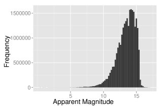
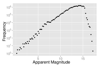
(a)	(b)
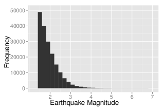
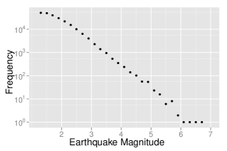
(c)	(d)

Figure 1: (a) Frequency of celestial bodies by apparent magnitude for 25 million celestial bodies in the Guide Star Catalog (GSC) 1.2 [24], (b) plotted on a log-linear scale. (c) Frequency of earthquakes by Richter magnitude for 20 years of California earthquakes, (d) plotted on a log-linear scale. Note that because the measurements are made on a logarithmic scale, the straight line in the log-linear plots implies that there is a power law at work.

Logarithmic scale measurements are not confined to the intensity of celestial bodies, however. Charles Richter’s scale [8, 27] for measuring earthquake magnitude is also logarithmic, and earthquake magnitude frequency follows an exponential distribution as well (see Fig. 1(c)–(d)). Moreover, as with astrophysical objects, range searching on geographic coordinates for earthquake occurrences is a common scientific query.

Similar in spirit to the Weber-Fechner Law, Zipf’s Law is an empirical statement about frequencies in real-world data sets. Zipf’s Law (e.g., see [18]) states that the frequency of a data value in real world data sets, such as words in documents, is inversely proportional to its rank. In other words, the relationship between frequency and rank follows a power law. For example, the popularity of web pages on the Internet follows such a distribution [5].

1.2 Problem Statement

Conventional range searching has no notion of priority. All points are considered equal and are dealt with equally. Nevertheless, as demonstrated by the Weber-Fechner Law and Zipf’s Law, there are many real-world applications where data points are not created equal—they are prioritized. We therefore aim to develop range query data structures that handle these priorities directly. Specifically, we seek to take advantage of prioritization in two ways: we would like query time to vary according to the priority of items affecting the query, and we want to allow for items beyond a priority threshold not to be involved in a given query.

Because of the above-mentioned laws, we feel we can safely sacrifice some granularity in item weight, focusing instead on their logarithm, to fulfill these goals. The ultimate design goal, of course, is that we desire data structures that provide meaningful prioritized responses but do not suffer the logarithmic slowdown or an increase in space that would come from treating priority as a full-fledged data dimension. To that end, given an item $x$, let us assume that it is given a priority, $p(x)$, that is positively correlated to $x$’s importance. So as to normalize item importance, if such priorities are already defined on a logarithmic scale (like the Richter scale), then we define $x$’s rank, $r(x)$, as $r(x)=\lfloor p(x)\rfloor$ and we define $x$’s weight, $w(x)$, as $w(x)=2^{p(x)}$. Otherwise, if priorities are defined on a uniform scale (like hyperlink in-degree on the World-wide web), then we define the $w(x)=p(x)$ and we define $r(x)={\left\lfloor\log{w(x)}\right\rfloor}$. We further assume that weight is polynomial in the number of inputs. This assumption implies that there are $O(\log n)$ possible ranks, and that $\log W/w=O(\log n)$, where $w$ is a weight polynomial in $n$ and $W$ is the sum of $n$ such weights. Given these normalized definitions of rank and weight, we desire efficient data structures that can support the following types of prioritized range queries:

• Threshold query: Given a query range, $R$, and a weight, $w$, report the points in $R$ with rank greater than or equal to ${\left\lfloor\log{w}\right\rfloor}$.

• Top-$k$ query: Given a query range $R$ and an integer, $k$, report the top $k$ points in $R$ based on rank.

1.3 Prior Work

As mentioned above, range reporting data structures are well-studied in the Computational Geometry literature (e.g., see the excellent surveys by Agarwal [2] and Agarwal and Erickson [3]). In ${\bf R}^{2}$, 2- and 3-sided range queries can be answered optimally using McCreight’s priority search tree [22], which uses $O(n)$ space and $O(\log n+k)$ query time. Using the range trees of Bentley [7], and the fractional cascading technique of Chazelle and Guibas [12], 4-sided queries can be answered using $O(n\log n)$ space and $O(\log n+k)$ time. In the RAM model of computation, 4-sided queries can be answered using $O(n\log^{\epsilon}n)$ space and $O(\log n+k)$ time [11]. Alstrup, Brodal, and Reuhe [4] further showed that range reporting in ${\bf R}^{3}$ can be done with $O(n\log^{1+\epsilon}n)$ space and $O(\log n+k)$ query time in the RAM model.

More recently, Dujmović, Howat, and Morin [15] developed a data structure called a biased range tree which, assuming that 2-sided ranges are drawn from a probability distribution, can perform 2-sided range counting queries efficiently. Afshani, Barbay, and Chan [1] generalized this result, showing the existence of many instance-optimal algorithms. Their methods can be viewed as solving an orthogonal problem to the one studied here, in other words, in that their points have no inherent weights in and of themselves and it is the distribution of ranges that determines their importance.

1.4 Our Results

Given a set $S$ of $n$ points in the plane, where each point $p$ in $S$ is assigned a weight $w(p)$ that is polynomial in $n$, we provide a data structure, called a priority range tree, which accommodates fast three-sided orthogonal range reporting queries. In particular, given a three-sided query range $R$ and a weight $w$, our data structure can be used to answer a threshold query, reporting all points $p$ in $R$ such that $\lfloor\log{w(p)}\rfloor\geq\lfloor\log{w}\rfloor$ in time $O(\log W/w+k)$, where $W$ is the sum of the weights of all points in $S$. In addition, we can also support top-$k$ queries, reporting $k$ points that have the highest $\lfloor\log{w(.)}\rfloor$ value in $R$ in time $O(\log\log n+\log W/w+k)$, where $w$ is the smallest weight among the reported points. The priority range tree data structure occupies linear space, and operates under the standard RAM model of computation. Then, with a well-known technique for converting a 3-sided range reporting structure into a 4-sided range reporting structure, we show how to construct a data structure for answering prioritized 4-sided range queries with similar running times to those for our 3-sided query structure. The space for our 4-sided query data structure is larger by a logarithmic factor.

1.5 A Note About Distributions

A key feature of the priority range tree is that it is distribution agnostic. This distinction is crucial, since if the distribution of priorities is fixed to be exponential, then a trivial data structure achieves the same results: for i = $1$ to ${\left\lfloor\log w_{\text{max}}\right\rfloor}$, create a priority search tree $P_{i}$ containing all points with weight $2^{i}$ and above. Because the distribution is exponential, the number of elements in $P_{i}$ is at most $n/{2^{i}}\leq W/{2^{i}}$, and hence, querying $P_{{\left\lfloor\log w\right\rfloor}}$ correctly answers the query and takes time $O(\log W/w+k)$. Furthermore, the space used for all data structures is $\sum_{i}n/2^{i}=O(n)$.

However, such a strategy does not work for other distributions (including power law distributions, which commonly occur in practice) since the storage for each data structure becomes too great to meet the desired query time and maintain linear space. Thus, our data structure provides query times approaching the information theoretic lower bound, in linear space, regardless of the distribution of the priorities.

2 Preliminary Data Structuring Techniques

In this section, we present some techniques that we use to build up our priority range tree data structure.

2.1 Weight-balanced Priority Search Trees

Consider the following one-dimensional range reporting problem: Given a set $S$ of $n$ points in ${\bf R}$, where each point $p$ has weight $w(p)$, we would like to preprocess $S$ into a data structure so that we can report all points in the query interval $[a,b]$ with weight greater or equal to $w$. Storing the points in a priority search tree [22], affords $O(\log{n}+k)$ query time using linear space. We can obtain a query time of $O(\log W/w+k)$ by ensuring that the priority search tree is weight balanced.

Definition 1

We say a tree is weight balanced if item $i$ with weight $w_{i}$ is stored at depth $O(\log W/w_{i})$, where $W$ is the sum of the weights of all items stored in the tree.

To build this search tree, we use a trick similar to Mehlhorn’s rule 2 [23]. We first choose the item with the highest weight to be stored at the root. We then divide the remaining points into two sets $A$ and $B$ such that the $x$-value of every point in $A$ is less than or equal to the $x$-value of every point in $B$ and ${\left\lvert\sum_{a\in A}w(a)-\sum_{b\in B}w(b)\right\rvert}$ is minimized. Finally, we store the maximum $x$ value from $A$ in the root to facilitate searching, and then recursively build the left and right subtrees on sets $A$ and $B$. We call this technique split by weight. Priority search trees are built much the same way, except that $A$ and $B$ are chosen to have approximately the same cardinality, which we call split by size.

The resulting search tree is both weight balanced and heap ordered by weight, and can therefore be used to answer range reporting queries with the same procedure as the priority search tree.

Lemma 1

The weight-balanced priority search tree consumes $O(n)$ space, and can be used to report all points in a query range $[a,b]$ with weight at least $w$ in time $O(\log(W/w)+k)$ where $W$ is the sum of the weights of all points in the tree.

2.2 Persistent Heaps

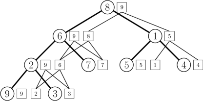
Figure 2: A persistent heap. Circular nodes represent the original binary tree and square nodes represent heaps at each step of the BuildHeap algorithm.

The well-known BuildHeap algorithm can transform any complete binary tree into a heap in linear time [17]. Using the node-copying method for making data structures persistent [14], we can maintain a record of the heap as it exists during each step of the BuildHeap algorithm, allowing us to store a heap on every subtree in linear space. We call this data structure a persistent heap.

Lemma 2

Let $T$ be a tree with $n$ nodes. If the BuildHeap algorithm runs in time $O(n)$ on $T$, then we can augment every node of $T$ with a heap of the elements in its subtree using extra space $O(n)$.

Proof

For each swap operation of the BuildHeap algorithm, we do not swap within the tree, but we create two extra nodes, add the swapped elements to these nodes, and add links to the heaps from the previous stages of the algorithm (see Fig. 2).

Given $n$ points in ${\bf R}^{2}$, this strategy can be used as a substitute for the priority search tree, by first building complete binary search tree on the $x$ values, and then building a persistent heap using the $y$ values as keys.

2.3 Layers of Maxima

We now turn our attention to the following two problems: Given $l$ points in ${\bf Z}_{m}\times{\bf R}$, preprocess the points into a data structure, to quickly answer the following queries.

1. Domination Query: Given a query point $(x,y)$, report all points $(p_{x},p_{y})$ such that $x\leq p_{x}$ and $y\leq p_{y}$.

2. Maximization Query: Given a query value $y$, report a point with the largest $x$-value, such that its $y$-value is greater than $y$.

This problem can be solved optimally using two techniques: we form the layers of maxima of the points and use fractional cascading to reduce search time.

A point $p\in{\bf R}^{2}$, dominates a point $q\in{\bf R}^{2}$ iff each coordinate of $p$ is greater than that of $q$. A point $p$ is said to be a maximum of a set $S$ iff no point in $S$ dominates $p$. Given a set $S$, if we find the set of maxima of $S$, remove the maxima and repeat, then the resulting sets of points are called the layers of maxima of $S$.

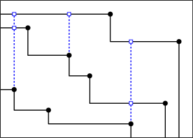
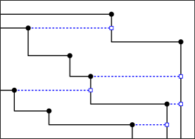
(a)	(b)

Figure 3: The layers of maxima with fractional cascading (a) from bottom to top and (b) from left to right.

We begin by constructing the layers of maxima of the $l$ points. We then form a graph from the layers of maxima by creating a vertex for each point and connecting vertices that are in the same layer in order by $x$ coordinate.

We first fractionally cascade the points from bottom to top, sending up every other point from one layer to the next, including points copied from previous layers (see Fig. 3(a)). We then repeat the same procedure, fractionally cascading the points from left to right (see Fig. 3(b)). For bottom-to-top fractional cascading, we create $m$ entry points into the top layer our data structure stored as an array indexed by $x$ value. Each entry point stores one pointer to the maxima in the top layer that succeeds it in $x$-value.

To answer domination queries, we enter the catalog at index $x$, reports all points on the current layer that match the query, then jump down to the next layer and repeat. Each answer can be found with a constant amount of searching. Therefore, the query takes time $O(\max\{k,1\})$ where $k$ is the output size.

To answer maximization queries, we create a catalog of $O(l)$ entry points on the right. Each entry point stores a pointer to a point (copied or not) on the top layer of maxima. Since the domain of $y$ is not constrained to the integers, we perform a search for our query $y$ among the entry points and immediately jump to our answer. This data structure gives us $O(l)$ space and $O(\log{l})$ query time.

We now have all the machinery to discuss the priority range tree data structure.

3 The Priority Range Tree

In this section, we present a data structure for three-sided range queries on prioritized points. We assume that each point $p$ has a weight $w(p)$, and we define $r(p)={\left\lfloor\log w(p)\right\rfloor}$ to be the rank of $p$. Given a range $R=[x_{1},x_{2}]\times[y,\infty)$ our data structure accommodates the following queries.

1. Threshold Queries: Given a query weight $w$, report all points $p$ in $R$ whose weight satisfies ${\left\lfloor\log{w(p)}\right\rfloor}\geq{\left\lfloor\log w\right\rfloor}$.

2. Top-$k$ Queries: Given an integer $k$, report the $k$ points in $R$ with the highest ${\left\lfloor\log{w(\cdot)}\right\rfloor}$ value.

We first describe a data structure that has significant storage requirements, to illustrate how to perform each query. We then show how to reduce the space requirements.

For our underlying data structure, we build up a weight-balanced priority search tree on the $x$-values of our points. On top of this tree, we build one persistent heap for each different rank. That is, given rank $r$, we build a persistent heap on the $y$-values of points that have rank $r$. Of course, points with different rank must be compared in this scheme, therefore, when building a persistent heap for rank $r$, we treat points with rank not equal to $r$ as dummies with $y$-value $-\infty$. Once we are done building up these persistent heaps, each node has $O(\log{n})$ heaps rooted at it, one for each rank. For each node, we store a catalog, which is an array of roots of each of the $O(\log n)$ heaps, indexed by rank. On top of each catalog, we build the fractionally-cascaded layers-of-maxima data structure, described in the previous section, storing a coordinate (rank, y-value) for each root of the $O(\log n)$ heaps.

3.1 Threshold Queries

We first search for $x_{1}$ and $x_{2}$ down to depth $O(\log W/w)$ in our weight-balanced priority search tree, checking each point for membership as we make our way down the tree.

Each node on the search paths to $x_{1}$ and $x_{2}$ may have left or right subtree whose $x$ values are entirely in the range $[x_{1},x_{2}]$. For each such subtree, we query the layers-of-maxima data structure to find all points in the catalog that dominate $({\left\lfloor\log w\right\rfloor},y)$. If any points are returned, then we perform a layer-by-layer search through the heaps stored for each rank. We return any points that satisfy the query $y$ value.

Each layers-of-maxima search can be charged to the search depth or an answer, and each search within a heap can be charged to an answer. Therefore, we get the desired running time of $O(\log W/w+k)$.

3.2 Top-$k$ Queries

This query type is slightly more involved, so we begin by describing how to find one point of maximum rank in a query range.

Max-reporting.

Given a range $R=[x_{1},x_{2}]\times[y,\infty)$, the max-reporting problem is to report one point in $R$ with maximum rank.

A first attempt is to search for $x_{1}$ and $x_{2}$, and run a maximization query for each layers-of-maxima data structure along the search path, maintaining the point in $R$ with maximum rank found so far. Although this is a correct algorithm, there are two issues with this approach, which are brought about because we do not have a query weight:

1. The search may reach depth $\omega(\log W/w^{\prime})$, where $w^{\prime}$ is the weight of the answer.

2. Each query to a layers-of-maxima data structure takes time $O(\log\log n)$.

Therefore, we maintain a depth limit, initially $\infty$, telling our algorithm when to stop searching. If there is no point in $R$, then our search reaches a leaf at depth $O(\log n)$ and stops. If we find a point $p$ in $R$, we decrease the depth limit to $c\log W/w(p)$, where $c$ is the constant hidden in the big-oh notation for the weight-balanced priority search tree. If our search reaches the depth limit, then there are no points with greater rank lower in the tree, and we can stop searching. Otherwise, every time we encounter point in $p^{\prime}$ in $R$ with higher rank $r^{\prime}={\left\lfloor\log w^{\prime}\right\rfloor}$ we decrease the depth limit to $c\log W/w^{\prime}$.

We reduce the layers-of-maxima query time by fractionally cascading the layers-of-maxima data structure across the entire search tree, allowing us to do one $O(\log\log n)$-time query in the root catalog, and $O(1)$ extra work in the catalogs on the search path.

With these two changes, the search takes time $O(\log\log n+\log W/w^{\prime})$ total ($O(\log n)$ if no such point exists).

Top-$k$ Reporting

We now extend the max-reporting algorithm to report $k$ points with highest rank in time $O(\log\log n+\log W/w^{\prime}+k)$ under the standard RAM model.

If the top $k$ points all have the same rank, then we can use our max-reporting algorithm to find the point with highest rank, and use the threshold queries to recover all $k$ points. However, if we have to find points with lower rank, we want to avoid doing an expensive search for each rank. We can accomplish this goal with a priority queue.

Perform an initial max-reporting search. Every point in $R$ encountered during our search is inserted into a priority queue with key equal to its rank. Along with each point we store a link back to the location in the layers-of-maxima data structure where it was found. When we finish the initial max-reporting query, we iterate the following process:

1. Remove the point $p$ with maximum rank $r$ from the priority queue.

2. Enter the layers-of-maxima data structure at point $p$, and insert both the predecessor of $p$ on the same layer and on the layer below into the priority queue. Each one of these points are candidates for reporting. We then mark points to ensure that duplicates are not added to the priority queue.

3. Search in the heap data structure where point $p$ was found, and report any additional points it contains that are in $R$ (without exceeding $k$ points).

4. If we have reported $k$ points then we are done. Otherwise, look at the point with maximum rank in the priority queue. If its rank $r^{\prime}={\left\lfloor\log{w^{\prime}}\right\rfloor}$ is less than $r$, then we increase our search depth to $c\log W/w^{\prime}$, and continue searching, adding points the priority queue as before.

This priority queue can be efficiently implemented in the standard RAM model. We store our priority queue as an array $P$, indexed by key. We store in cell $P[r]$ a linked list of elements with key $r$. Additionally, we maintain two values, $r_{\text{max}}$ and $r_{\text{min}}$, which is the maximum (minimum) key, of all elements in the priority queue. We insert an item with key $k$, by adding it to the linked list $P[k]$ in $O(1)$ time, and updating $r_{\text{max}}$ and $r_{\text{min}}$. To remove an item with the maximum key $k$, we remove it from the linked list $P[k]$. If $P[k]$ becomes empty, then we update $r_{\text{max}}$ (and possibly $r_{\text{min}}$).

We now show that our top-$k$ reporting algorithm has running time $O(\log\log n+\log W/w^{\prime}+k)$. We spend an initial $O(\log\log n)$-time search for our fractional cascading. Our initial search and subsequent extensions of the search path takes time $O(\log W/w^{\prime})$, by virtue of our depth limit. For each heap in which we perform a layer-by-layer search, we can charge the search time to answers reported. All that remains to be shown is that the priority queue operations do not take too much time.

For each point discovered in a layers-of-maxima query along the search path, we perform at most one insert into the priority queue, thus we do $O(\log W/w^{\prime})$ of these insertions into the priority queue, each one taking constant time. Furthermore, we can charge all of our priority queue remove operations (excluding pointer updates) to answers. Updating the priority queue pointers does not negatively impact the running time, since the total number of array cells we march through to do the pointer updates is $O(\log W/w^{\prime})$. For each remove operation, we may perform up to two subsequent insertions, which we can charge to answers. Therefore, we get a total running time of $O(\log\log n+\log W/w^{\prime}+k)$.

As described, the priority range tree consumes $O(n\log^{2}n)$ space, since each persistent heap may consume $O(n\log n)$ space and we store $O(\log n)$ such persistent heaps.

3.3 Reducing the Space Requirements

We can reduce the space to $O(n)$ by making several modifications to the search tree. We build our underlying tree using the split-by-weight strategy down to depth $\frac{1}{2}\log{n}$, then switch to a split-by-size strategy for the deeper elements, forcing these split-be-size subtrees to be complete. By switching strategies we do not lose the special properties that we desire: the tree is still weight balanced and heap ordered on weights. Finally, we do not store auxiliary data structures for split-by-size subtrees with between $\frac{1}{2}\log{n}$ and $2\log{n}$ elements in them, we only store one catalog for each such subtree. We call these subtrees buckets.

Lemma 3

The priority range tree consumes $O(n)$ space.

Proof

Each layers-of-maxima data structure uses $O(\log n)$ storage. We store one such data structure with each split-by-weight node and one for each split-by-size node excepting those in subtrees with between $1/2\log n$ and $2\log n$ elements. There are $O(\sqrt{n})$ split-by-weight nodes, since they are all above depth $1/2\log n$. Each subtree $T_{i}$ rooted at depth $1/2\log n$ of size $n_{i}$ will have at most $2n_{i}/\log n$ nodes that store the auxiliary data structure. Therefore, the total space for layers-of-maxima data structures is $O(\sqrt{n}\log n)+\sum_{i}O(n_{i}/\log n)O(\log n)=O(n)$.

For the persistent heaps, we ensure that each subtree $T_{i}$ rooted at depth $1/2\log n$ is complete, on which we know BuildHeap will run in linear time. If $T_{i}$ contains fewer than $1/2\log n$ nodes, then $T_{i}$ has $O(\log n)$ heap nodes. Otherwise, each subtree $T_{i}$ stores $O(n_{i}/\log n)$ heap nodes per rank.

Each node above depth $1/2\log n$ can contribute $O(\log{n})$ swaps for each heap. Each heap therefore requires $O(\sqrt{n}\log n+\sum_{i}n_{i}/\log{n})=O(n/\log{n})$ space. Since we have $O(\log{n})$ heaps, our data structure requires $O(n)$ space.

These structural changes affect our query procedures. In particular, there are three instances where the bucketing affects the query:

1. If the initial search phase hits a bucket, then we exhaustively test the $O(\log n)$ points in the bucket. We only reach a bucket if the search path is of length $\Omega(\log n)$ and therefore we can amortize this exhaustive testing over the search.

2. If we reach a bucket during our layer-by-layer search through a heap, then exhaustively searching through the bucket is not an option, as this would take too much time. Instead, we augment the layers-of-maxima data structure for the bucket so we can walk through lower $y$ values with the same rank as the maxima (possibly producing duplicates).

3. By the very nature of the BuildHeap algorithm, it is possible that points in $R$ were DownHeaped into the buckets, and that information is also lost. Therefore, when looking layer by layer through the heaps we also need to test for membership of the tree nodes in addition to the heap nodes (also possibly producing duplicates).

Each point matching the query will be encountered at most three times, once in each search phase. Therefore, we can avoid returning duplicates with a simple marking scheme without increasing the reporting time by more than a constant factor.

Theorem 3.1

The priority range tree consumes $O(n)$ space and can be used to answer three-sided threshold reporting queries with rank above ${\left\lfloor\log w\right\rfloor}$ in time $O(\log W/w+k)$, and top-$k$ reporting queries in time $O(\log\log n+\log W/w^{\prime}+k)$, where $W$ is the sum of the weights of all points in $S$, $w^{\prime}$ is the smallest weight of the reported points, and $k$ is the number of points returned by the query.

4 Four-sided Range Reporting

Our techniques can be extended to four-sided range queries with an added logarithmic factor in space using a twist on a well-known transformation. Given a set $S$ of points in ${\bf R}^{2}$, we form a weight-balanced binary search tree on the $x$-values of the points, such that the points are stored in leaves (e.g., a biased search tree [6]). For each internal node, we store the range of $x$-values of points contained in its subtree. For each internal node $x$ (except the root), we store a priority range tree $P_{x}$ on all points in the subtree: if $x$ is a left child then $P_{x}$ answer queries of the form $[a,\infty)\times[c,d]$, if $x$ is a right child then $P_{x}$ answers queries of the form $(-\infty,b]\times[c,d]$. We can answer four-sided query given the range $[a,b]\times[c,d]$, by doing the following:

We first search for $a$ and $b$ in in the weight-balanced binary search tree. Let $s$ be the node where the search for $a$ and $b$ diverges, then $a$ must be in $s$’s left subtree $\text{left}(s)$ and $b$ must be in $s$’s right subtree $\text{right}(s)$. Then we query $P_{\text{left}(s)}$ for points in $[a,\infty)\times[c,d]$ and query $P_{\text{right}(s)}$ for points in $(-\infty,b]\times[c,d]$ and merge the results. In the case of top-$k$ queries, we must carefully coordinate the search and reporting in each priority range tree, otherwise we may search too deeply in one of the trees or report incorrect points.

5 Conclusion

Our priority range tree data structure can be used to report points in a three-sided range with rank greater than or equal to ${\left\lfloor\log w\right\rfloor}$ in time $O(\log W/w+k)$, and report the top $k$ points in time $O(\log\log n+\log W/w^{\prime}+k)$, where $w^{\prime}$ is the smallest weight of the reported points, using linear space. These query times extend to four-sided ranges with a logarithmic factor overhead in space. Our results are possible because of our reasonable assumptions that the weights are polynomial in $n$, and that the magnitude of the weights, rather than the specific weights themselves, are more important to our queries.

Acknowledgments.

This work was supported in part by NSF grants 0724806, 0713046, 0830403, and ONR grant N00014-08-1-1015.

References

- [1] Afshani, P., Barbay, J., Chan, T.M.: Instance-optimal geometric algorithms. In: Proc. 5th IEEE Symposium on Foundations of Computer Science. pp. 129–138. (2009)
- [2] Agarwal, P.K.: Range searching. In: Goodman, J.E., O’Rourke, J. (eds.) Handbook of Discrete and Computational Geometry, pp. 575–598. CRC Press LLC, Boca Raton, FL (1997)
- [3] Agarwal, P.K., Erickson, J.: Geometric range searching and its relatives. In: Chazelle, B., Goodman, J.E., Pollack, R. (eds.) Advances in Discrete and Computational Geometry, Contemporary Mathematics, vol. 223, pp. 1–56. AMS, Providence, RI (1999)
- [4] Alstrup, S., Stolting Brodal, G., Rauhe, T.: New data structures for orthogonal range searching. In: Proc. 41st IEEE Symposium on Foundations of Computer Science. pp. 198–207 (2000)
- [5] Baeza-Yates, R., Castillo, C., López, V.: Characteristics of the web of spain. International Journal of Scientometrics, Informetrics, and Bibliometrics 9 (2005)
- [6] Bent, S.W., Sleator, D.D., Tarjan, R.E.: Biased search trees. SIAM J. Comput. 14, 545–568 (1985)
- [7] Bentley, J.L.: Multidimensional divide-and-conquer. Commun. ACM 23(4), 214–229 (1980)
- [8] Boore, D.: The Richter scale: its development and use for determining earthquake source parameters. Tectonophysics 166, 1–14 (1989)
- [9] Brin, S., Page, L.: The anatomy of a large-scale hypertextual web search engine. Comput. Netw. ISDN Syst. 30(1-7), 107–117 (1998)
- [10] Chazelle, B.: Filtering search: a new approach to query-answering. SIAM J. Comput. 15, 703–724 (1986)
- [11] Chazelle, B.: A functional approach to data structures and its use in multidimensional searching. SIAM J. Comput. 17(3), 427–462 (1988)
- [12] Chazelle, B., Guibas, L.J.: Fractional cascading: I. A data structuring technique. Algorithmica 1(3), 133–162 (1986)
- [13] Dehaene, S.: The neural basis of the Weber-Fechner law: a logarithmic mental number line. Trends in Cognitive Sciences 7(4), 145–147 (2003)
- [14] Driscoll, J.R., Sarnak, N., Sleator, D.D., Tarjan, R.E.: Making data structures persistent. Journal of Computer and System Sciences 38(1), 86–124 (1989)
- [15] Dujmović, V., Howat, J., Morin, P.: Biased range trees. In: Proc. 19th ACM-SIAM Symposium on Discrete Algorithms. pp. 486–495. SIAM, Philadelphia, PA, USA (2009)
- [16] Evans, J.: The history & practice of ancient astronomy. Oxford University Press (Oct 1998)
- [17] Floyd, R.W.: Algorithm 245: Treesort 3. Commun. ACM 7(12), 701 (1964)
- [18] Frakes, W.B., Baeza-Yates, R. (eds.): Information retrieval: data structures and algorithms. Prentice-Hall, Inc., Upper Saddle River, NJ, USA (1992)
- [19] Fries, O., Mehlhorn, K., Näher, S., Tsakalidis, A.: A data structure for three-sided range queries. Inform. Process. Lett. 25, 269–273 (1986)
- [20] Hecht, S.: The visual discrimination of intensity and the Weber-Fechner law. Journal of General Physiology 7(2), 235–267 (1924)
- [21] Lueker, G.S.: A data structure for orthogonal range queries. In: Proc. 19th IEEE Symposium on Foundations of Computer Science. pp. 28–34 (1978)
- [22] McCreight, E.M.: Priority search trees. SIAM J. Comput. 14(2), 257–276 (1985)
- [23] Mehlhorn, K.: Nearly optimal binary search trees. Acta Informatica 5(4), 287–295 (1975)
- [24] Morrison, J., Roser, S., McLean, B., Bucciarelli, B., Lasker, B.: The guide star catalog, version 1.2: An astronomic recalibration and other refinements. The Astronomical Journal 121, 1752–1763 (2001)
- [25] Overmars, M.H.: Efficient data structures for range searching on a grid. J. Algorithms 9, 254–275 (1988)
- [26] Page, L., Brin, S., Motwani, R., Winograd, T.: The PageRank citation ranking: Bringing order to the web. Technical Report 1999-66, Stanford InfoLab (November 1999), http://ilpubs.stanford.edu:8090/422/, previous number = SIDL-WP-1999-0120
- [27] Richter, C.F.: Elementary Seismology. W.H. Freeman and Co. (1958)
- [28] Satterthwaite, G.E.: Encyclopedia of Astronomy. Hamlyn (1970)