Finite-temperature phase transition to $m=1/2$ plateau phase in a S=1/2 XXZ model on Shastry-Sutherland Lattices

Abstract

We study the finite-temperature transition to the $m=1/2$ magnetization plateau in a model of interacting $S=1/2$ spins with longer range interactions and strong exchange anisotropy on the geometrically frustrated Shastry-Sutherland lattice. This model was shown to capture the qualitative features of the field-induced magnetization plateaus in the rare-earth tetraboride, ${\rm TmB_{4}}$. Our results show that the transition to the plateau state occurs via two successive transitions with the two-dimensional Ising universality class, when the quantum exchange interactions are finite, whereas a single phase transition takes place in the purely Ising limit. To better understand these behaviors, we perform Monte Carlo simulations of the classical generalized four-state chiral clock model and compare the phase diagrams of the two models. Finally, we estimate a parameter set that can explain the magnetization curves observed in ${\rm TmB_{4}}$. The magnetic properties and critical behavior of the finite-temperature transition to the $m=1/2$ plateau state are also discussed.

I INTRODUCTION

Geometrically frustrated interactions and quantum fluctuation inhibit the stabilization of classical orderings. They sometimes become a trigger for the emergence of several exotic orders such as, quantum spin ice on the pyrochlore latticeOnoga , spin liquid state on the honeycomb latticeMeng , and multiple magnetization plateausSebastian . Therefore, quantum spin systems with frustrated interactions have attracted great interest from both theoretical and experimental approaches.

The $S=1/2$ antiferromagnetic Heisenberg spin model on the Shastry-Sutherland lattice (SSL)SSL is one of such systems. The Hamiltonian can be expressed by the nearest neighbor (intradimer) $J$ and the next nearest neighbor (interdimer) $J^{\prime}$ couplings:

$${\mathcal{H}} = J\sum_{\rm N.N.}{\bf S}_{i}\cdot{\bf S}_{j}+J^{\prime}\sum_{\rm N.N.N.}{\bf S}_{i}\cdot{\bf S}_{j}.$$ (1)

Experimentally, $\rm{SrCu(BO_{3})_{2}}$Kageyama1 ; Kageyama2 has been studied extensively for its realization of the model. In this compound, ${\rm CuBO_{3}}$ layers stack along the $c$-axis direction and each magnetic layer consists of ${\rm Cu^{2+}}$ ions carrying $S=1/2$ spins arranged in an orthogonal dimer structure that is topologically equivalent to the SSL. From several experimental observations, it was confirmed that the field dependence of the magnetization exhibits multiple magnetization plateaus. In these magnetization plateau states, Wigner crystals of spin-triplet dimersTakigawa are realized reflecting the strong competition between the kinetic energy gain and mutual repulsion of the dimers.

Theoretically, this model has been studied in great detailUeda and several states, such as the plaquette singlet state at zero fieldKoga ; Lauchil and a spin supersolid state in the magnetic fieldsMomoi were predicted. In a recent paper by Sebastian et al.Sebastian , the possibility of fractional magnetic plateaus was discussed in analogy to the quantum Hall effect.

Fractional magnetic plateaus have recently been discovered at low temperatures in rare-earth tetraborides $\rm{RB_{4}}$ [R is a rare-earth element]TbB4 ; ErB4 ; TmB4_1 ; TmB4_2 ; TmB4_3 ; TmB4_4 ; Siemensmeyer . The magnetic moment carrying ${\rm R^{3+}}$ ions in these compounds are arranged in a SSL in the $ab$-plane. In ${\rm TmB_{4}}$, an extended magnetization plateau at $m=1/2$ was confirmed for $H_{c1}\sim 1.9$[T]$<H<H_{c2}\sim$ 3.6[T] when a magnetic field is applied along the $c$-axisTmB4_1 ; TmB4_2 . Here $m$ is the normalized value by the saturation magnetization, $m=m_{z}/m_{s}$. In contrast to $\rm{SrCu(BO_{3})_{2}}$ a strong anisotropy along the $c$-axis is expected owing to the crystal fields. From specific heat measurementsTmB4_2 , it has been suggested that the degeneracy of the $J$=$6$ multiplet of ${\rm Tm^{3+}}$ is lifted - the lowest energy state for a single ion is the non-Kramers doublet with $J_{z}$=$\pm 6$ and there exists a large energy gap to the first excited doublet. By restricting the local Hilbert space to the lowest energy doublet, the low-energy magnetic properties of the material can be described by a S=1/2 XXZ model with Ising-like exchange anisotropy and a ferromagnetic transverse coupling as discussed in the next section.

The magnetization curves for the effective Hamiltonian have already been calculatedMeng_Wessel ; Chang_Yang ; Liu . The effective Hamiltonian is the $S=1/2$ Ising-like XXZ model on the SSL and it is described by

$${\mathcal{H}} = \sum_{\rm N.N.}\left(J{\bf S}_{i}\cdot{\bf S}_{j}\right)_{\Delta_{\perp}}+\sum_{\rm N.N.N.}\left(J^{\prime}{\bf S}_{i}\cdot{\bf S}_{j}\right)_{\Delta_{\perp}}$$ (2)

$$- g\mu_{B}H\sum_{i}{S_{i}}^{z},$$

where $\Delta_{\perp}$ denotes the Ising anisotropy and $(J_{ij}{\bf S}_{i}\cdot{\bf S}_{j})_{\Delta_{\perp}}=-|J_{ij}|{\Delta}_{\perp}\left(S_{i}^{x}S_{j}^{x}+S_{i}^{y}S_{j}^{y}\right)+J_{ij}S_{i}^{z}S_{j}^{z}$. In the Ising limit $\Delta_{\perp}=0$, it has been established by several approaches - such as Monte Carlo simulations Meng_Wessel and tensor renormalization-group analysisChang_Yang - that only $m=1/3$ plateau is stabilized. The presence of the $m=1/2$ plateau has been confirmed when quantum spin fluctuation is includedMeng_Wessel ; Liu , and the ground-state phase diagram for $\Delta_{\perp}>0$ has been calculated. However, even for finite $\Delta_{\perp}$, the $m=1/3$ plateau phase extends over a wider range of applied fields than the $m=1/2$ plateau phase. Since the $m=1/3$ plateau is not observed in $\rm{TmB_{4}}$, the above Hamiltonian is insufficient to explain the experimental observations in ${\rm TmB_{4}}$.

In a previous letterSuzuki , we argued that ferromagnetic $J_{4}$ and antiferromagnetic $J_{3}$ couplings (see Fig. 1) are necessary to explain the stabilization of an extended $m=1/2$ plateau in the absence of the $m=1/3$ plateau. We also investigated the finite-temperature phase transition to the $m=1/2$ plateau state. The results of finite-size scaling analysis indicated that a two-step second-order transition takes place - the difference between two critical temperatures is within 0.5% of $J$. The universality class at both critical points is explained by the critical exponents of the two-dimensional Ising model.

For the finite-temperature transition, a nontrivial question remains unanswered. In the $m=1/2$ plateau phase, the lowest energy state is four-fold degenerate. Therefore, it is naively expected that the universality class should be the same as that of the four-state Potts model. As we discuss in this paper, the critical behavior can indeed be explained by the four-state Potts universality in the Ising limit, while the quantum spin model shows a two-step transition with both transitions belonging to the two-dimensional Ising universality class. Hence the phase diagrams for the thermal phase transitions for the two are different although both models possess the same symmetry. The low energy behavior of the $m=1/2$ plateau is shown to be described by the generalized four-state chiral clock model. As far as we know, the finite-temperature transition of the generalized chiral four-state clock model has not been studied precisely. Therefore, clarification of the finite-temperature transition to the $m=1/2$ plateau phase is also valuable from the view point of statistical mechanics. In the present paper, we discuss the properties of the model introduced in our previous letter in greater details, and clarify the nature of the phase transitions to the $m=1/2$ plateau state.

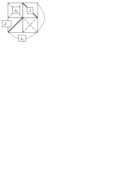
Figure 1: Effective model on the SSL with diagonal coupling $J$, nearest-neighbor coupling $J^{\prime}$, and additional couplings $J_{3}$ and $J_{4}$.

This paper is organized as follows. In section II, we reproduce the derivation of an effective Hamiltonian that captures the unique magnetization features in ${\rm TmB_{4}}$. An approach from the Ising limit of the effective Hamiltonian shows that $J_{4}$ couplings are important to stabilize the $m=1/2$ plateau state. In section III, we focus on the finite-temperature properties of the effective model and re-investigate the universality class of the transition to the $m=1/2$ plateau phase by extensive quantum Monte Carlo simulations. We show that the critical properties of the quantum model is different from those in the Ising limit. In section IV, a classical model, the generalized chiral four-state clock model, is proposed in order to understand the critical behavior of the original model. From Monte Carlo simulations, we find that the topology of the phase diagram for the classical model is the same as that of the original model. In comparison with the phase diagram for the classical model, we discuss the effects of quantum exchange on the finite-temperature transition. In section V, we discuss the magnetic properties of ${\rm TmB_{4}}$ and predict the critical properties of the finite-temperature transition to the $m=1/2$ plateau phase. Sec. VI is devoted to a summary of the results.

II EFFECTIVE MODEL

In this section, we derive the effective model for the low energy part of magnetic properties of ${\rm TmB_{4}}$ again. As discussed in the introduction, the ground state of the single ${\rm Tm^{3+}}$ ions is a $J_{z}=\pm 6$ doublet with a large energy gap between the first excited doublet. At low temperatures (compared to this energy gap), one can ignore the contributions from the higher multiplets and the low energy properties of the material are well described by an effective two-state model consisting of the $J_{z}=\pm 6$ doublet. The fact that the interactions between the moments are derived from itinerant electrons enables us to expect isotropic type (Heisenberg type) interactions. Therefore, we start from the Hamiltonian, $H_{eff}^{\prime}=H_{o}+H^{\prime}$, where $H_{o}=-D\sum_{i}(J_{i}^{z})^{2}$, $H^{\prime}=\sum_{\langle ij\rangle}G_{ij}{\bf J}_{i}{\bf J}_{j}$, and $0<|G_{ij}|\ll D$, where $G_{ij}$ is the coupling constant between two moments on the site $i$ and $j$, and $D$ is the easy-axis anisotropy from the crystal fields. By treating $H_{o}$ as the biggest term, we find that there are four degenerate states, namely $|J_{i}^{z},J_{j}^{z}\rangle=|6,6\rangle$, $|-6,6\rangle$, $|6,-6\rangle$, and $|-6,-6\rangle$, in the lowest energy level. We apply perturbation theory for $H_{eff}^{\prime}$ and calculate the matrix elements among these four states. The Hamiltonian for arbitrary moment pairs can be described by the $S=1/2$ Ising-like XXZ Hamiltonian, $h_{ij}=\left(J_{ij}{\bf S}_{i}\cdot{\bf S}_{j}\right)_{\Delta_{\perp}}$, where $(J_{ij}{\bf S}_{i}\cdot{\bf S}_{j})_{\Delta_{\perp}}=-|J_{ij}|{\Delta}_{\perp}\left(S_{i}^{x}S_{j}^{x}+S_{i}^{y}S_{j}^{y}\right)+J_{ij}S_{i}^{z}S_{j}^{z}$. Most importantly, the matrix elements for the transverse coupling ($\langle 6,-6|H^{\prime}|-6,6\rangle$ and $\langle-6,6|H^{\prime}|6,-6\rangle$) are proportional to $-\{G_{ij}/(-D)\}^{2J}$. Consequently, if the magnetic moment $J$ is even, the transverse coupling always becomes ferromagnetic. (Note that the longitudinal component of the interaction becomes ferromagnetic or antiferromagnetic depending on the sign of $G_{ij}$.)

The interaction $G_{ij}$ is expected to be the RKKY type, because this compound is a metal. Therefore, the effect of the long-range interactions is significant when the magnetic properties of ${\rm TmB_{4}}$ are considered. The principal interactions necessary to reproduce the dominant features of magnetization in ${\rm TmB_{4}}$ - in addition to the conventional SSL model with $J$ and $J^{\prime}$ couplings - are the $J_{3}$ and $J_{4}$ couplings, shown in Fig. 1 (f). There is another coupling with shorter range than that of $J_{3}$ and $J_{4}$ - the next-nearest neighbor coupling $J_{2}$ that is orthogonal to $J$ in the plaquettes with the diagonal interactions in the original SSL model. However, as we show in the following analysis, $J_{2}$ is not efficient in stabilizing the $m=1/2$ plateau state, because it stabilizes the $m=1/3$ plateau at the same time.

The Hamiltonian considered here is described by

$${\mathcal{H}} = \sum_{\langle i,j\rangle}\left(J{\bf S}_{i}\cdot{\bf S}_{j}\right)_{\Delta_{\perp}}+\sum_{\langle i,j\rangle^{\prime}}\left(J^{\prime}{\bf S}_{i}\cdot{\bf S}_{j}\right)_{\Delta_{\perp}}$$ (3)

$$+ \sum_{\langle i,j\rangle^{\prime\prime}}\left(J_{3}{\bf S}_{i}\cdot{\bf S}_{j}\right)_{\Delta_{\perp}}+\sum_{\langle i,j\rangle^{\prime\prime\prime}}\left(J_{4}{\bf S}_{i}\cdot{\bf S}_{j}\right)_{\Delta_{\perp}}$$

$$- g\mu_{B}H\sum_{i}{S_{i}}^{z},$$

where $\langle ij\rangle$, $\langle ij\rangle^{\prime}$, $\langle ij\rangle^{\prime\prime}$, and $\langle ij\rangle^{\prime\prime\prime}$ denote sums over all pairs on the bonds with the $J$, $J^{\prime}$, $J_{3}$, and $J_{4}$ couplings, respectively. The positive (negative) sign of each coupling denotes antiferromagnetic (ferromagnetic) interaction. The original SSL model interactions are always assumed to be antiferromagnetic, i.e., $J>0$ and $J^{\prime}>0$. In the following, we set $J$ as the unit of energy and express all the parameters of the model in units of $J$. We studied the above model on square lattices of the form $L\times L$ with periodic boundary conditions.

When $\Delta_{\perp}\ll 1$, the magnetic properties of the Hamiltonian (3) are qualitatively explained by considering the Ising limit ($\Delta_{\perp}=0$). At $J_{3}=J_{4}=0$, there are two candidates of the ground states at $m=m_{z}/m_{s}=2N^{-1}\sum_{i}{S^{z}}_{i}=0$, where $N=L^{d}$ and $d=2$. For $J^{\prime}/J<0.5$, each spin pair located on the diagonal bond $J$ forms an antiferromagnetic $classical$ dimer (ACD) (Fig. 2 (a)), but macroscopic degeneracy remains due to cancellations among interactions on the coupling $J^{\prime}$. The local energy of such state can be estimated as $E_{ACD}=-J/8$. In the other limit $J^{\prime}/J\gg 1$, the system approaches the antiferromagnetic Ising model on the square lattice, and the Néel state becomes the ground state (Fig. 2 (b)). The local energy of the Néel state is calculated as $E_{Neel}=J/8-J^{\prime}/2$. As is expected, the energy levels of the two states cross at $J^{\prime}/J=0.5$ and $T=0$, and the system shows a phase transition at the point. The local energies of the $1/2$ and $1/3$ plateau state are estimated in the same manner. The spin configurations in Fig. 2 (c) and (d) are realized in the $1/3$ and $1/2$ plateau phase, respectively. (These configurations were also confirmed from the snapshot of spin configuration in the Monte Carlo simulations in our previous studySuzuki .) From the spin configurations, we obtain $E_{1/3}=-J/24-J^{\prime}/6-H/6$ and $E_{1/2}=-H/4$, where $E_{1/3}$ and $E_{1/2}$ denote the local energy of the $1/3$ and $1/2$ plateau state. Since the energy of the fully polarized state is given by $E_{F}=J/8+J^{\prime}/2-H/2$, the magnetization curve shows a jump from the $m=1/3$ to $m=1$ at $H_{c}=J/2+2J^{\prime}$. We show the field dependence of local energy for these five states in Fig. 3. The energies of the $m=1/2$ and $m=1/3$ plateaus, and the fully polarized state are always degenerate at the saturation field $H_{c}$. Consequently, the degeneracy between these three states should be lifted when the additional couplings $J_{3}$ and $J_{4}$ are included. By estimating the energy gains due to $J_{3}$ and $J_{4}$, we find that the ferromagnetic $J_{4}$ coupling is one of the most efficient ways to stabilize the $1/2$ plateau Footnote . This analysis further demonstrates that the coupling $J_{2}$, which is perpendicular to the diagonal coupling $J$, does not stabilize the $m=1/2$ plateau, because the number of antiparallel spin pairs on the $J_{2}$ couplings equals that of the parallel ones. Hence this coupling was not included in the effective Hamiltonian.

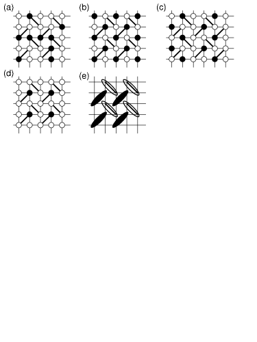
Figure 2: Conventional spin configurations in (a) an antiferromagnetic classical dimer (ACD) state, (b) the Néel state, (c) 1/3 plateau state, and (d) 1/2 plateau state. Solid and open circles indicate down and up spins respectively. (e) Schismatic spin configuration of $C_{2}$-symmetric phase (see text). Solid (open) ellipses mean spin pairs having the total magnetization $S^{z}\sim 0$ ($S^{z}\sim 1$).

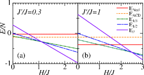
Figure 3: (color online) Field dependence of the local energy for the Ising limit.

III Quantum Monte Carlo Simulations

The qualitative discussion of the previous section is supplemented by large scale numerical simulation of the underlying model. We developed a variant of the standard Stochastic-Series-Expansion quantum-Monte-Carlo method based on the modified directed-loop algorithm to treat the longer-range interactions efficiently. KatoYasu ; Todo Using this new algorithm, simulations of the Hamiltonian (3) were performed on square lattices $L\times L$. Note that the negative sign problem does not appear in the quantum Monte Carlo computations for the Hamiltonian (3), because the transverse coupling is ferromagnetic as discussed in the previous section.

Fig. 4 shows the magnetization curves up to $L=40$, for different values of the ratio $J^{\prime}/J$, and how the curves evolve upon the introduction of ferro- and antiferro-magnetic $J_{4}$. In the computations, we fixed the $J_{4}$ coupling constant at $|J_{4}/J|=(1/\sqrt{2})^{3}\times J^{\prime}/J\sim 0.106$ and the Ising anisotropy $\Delta_{\perp}$ at $\Delta_{\perp}=0.2$.

At $J_{3}=J_{4}=0$, two magnetization plateaus appear at $m=1/2$ and 1/3, consistent with previous studies Meng_Wessel ; Liu ; Chang_Yang . When the longitudinal component of $J_{4}$ coupling is ferromagnetic, the system shows a strong tendency towards the stabilizing an extended plateau at $m=1/2$. Snapshots of the Monte Carlo simulations in the $m=1/2$ plateau phase confirm the realization of spin configuration shown in Fig. 2 (d). As long as there is the finite ferromagnetic $J_{4}$ coupling, the $m=1/3$ plateau region shrinks, for all values of the ratio $J^{\prime}/J$. This follows naturally from the analysis of the Ising spin model discussed above. In the Ising limit, the field extent of the $m=1/2$ plateau expands by an amount proportional to 4$|J_{4}|/J$, while that of the $m=1/3$ plateau contracts by an amount proportional to 6$|J_{4}|/J$.

When the longitudinal component of $J_{4}$ coupling is antiferromagnetic both $m=1/2$ and $1/3$ plateaus disappear. For antiferromagnetic $J_{4}$, no conclusive evidence of any plateaus has been obtained in our calculations except for $J^{\prime}/J=0.5$. A feature appears in the magnetization curve around $m=1/4$ for $J^{\prime}/J=0.5$. Fig. 5 (a) shows the expansion of the magnetization curve around $H\sim 0.75$ for $J^{\prime}/J=0.5$. For $0.60<H/J<0.74$, the magnetization curve becomes flat at $m=2/9$. Significantly, the $m=2/9$ plateau was also obtained for the parent Shastry-Sutherland model and observed in ${\rm SrCu(BO_{3})_{2}}$.Sebastian To identify the spin structure, we calculated the spin-spin and the bond-spin correlation functions. (As for the definition of bond spins, please see eq. (4)) The results are shown in Fig. 5 (b) and (c), respectively. In this plateau region, the $3\sqrt{2}\times 3\sqrt{2}$ structure accompanying $90\,^{\circ}$ rotational symmetry breaking is clearly stabilized. This is the same symmetry breaking as the $m=1/2$ plateau state. This plateau state has a characteristic feature: the periodicity of the $m=2/9$ plateau state is longer than the distance of $J_{4}$ couplings. Furthermore, the periodicity of this plateau is the same as that discussed in ref. Mila , but the precise spin configuration is a little bit different from their results shown in figure 5 in ref. Mila because the magnitude of the moments on the qlaquette without the diagonal bonds is lager than that on the diagonal bonds having total $S^{z}=1$.

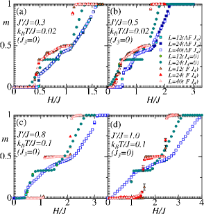
Figure 4: Magnetization curves when $J_{4}/J=(1/\sqrt{2})^{3}J^{\prime}/J$ (color online) and $\Delta_{\perp}=0.2$. Circles indicate the results at $J_{4}=0$ case. Triangles and squares are the results of the ferromagnetic and antiferromagnetic longitudinal $J_{4}$ couplings, respectively. All symbols accompany error bars, which are smaller than the symbol size (here and the following figures).

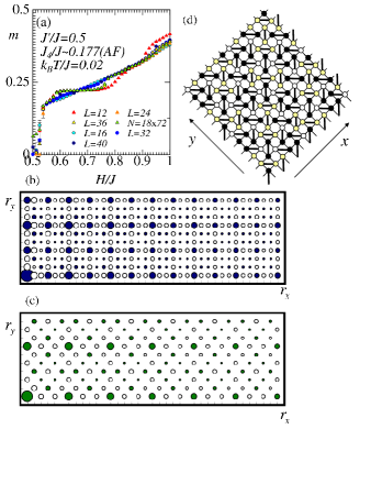
Figure 5: (color online) (a) Magnetization curves when $J^{\prime}/J=0.5$ and the antiferromagnetic $J_{4}/J=(1/\sqrt{2})^{3}J^{\prime}/J$. (b) and (c) are results for spin-spin and bond-spin correlations at $k_{B}T/J=0.02$. Colored (open) circles correspond to the positive (negative) amplitude. The area of circles is proportional to the amplitude. Error bars are smaller than the symbol sizes. (d) Schematic spin configuration in the $m=2/9$ plateau state. Solid circles denote up spins. Yellow circles surrounded by up spins are occupied by up or down spins with almost equal probability.

In the following, we focus on the finite-temperature transition to the $m=1/2$ plateau state. The snapshot of the spin configuration of the $m=1/2$ plateau phase leads us to expect the $90\,^{\circ}$ ($C_{4}$) rotation symmetry breaking around the center of the plaquette without diagonal coupling $J$. In context of the bare spin language, the universality class of the finite-temperature transition is expected to be the four-state Potts universality class because the lowest energy state in the $m=1/2$ plateau is four-fold degenerate. However, the other scenario is also possible for $\Delta_{\perp}\neq 0$ because the group $C_{4}$ has a subgroup $C_{2}$. By introducing the $90\,^{\circ}$ lattice rotation “$c_{4}$” around the center, we can express the symmetry group in the paramagnetic phase as $C_{4}=\{e,c_{4},c_{4}^{2},c_{4}^{-1}\}$. If the system exhibits a two-step phase transition, the symmetry breaks down to $\{e,c_{4}^{2}\}$ at the higher critical temperature $T_{c1}$, and the remaining symmetry breaks down to the trivial group $\{e\}$ at the lower critical temperature $T_{c2}$.

To investigate the symmetry breaking at the critical point, we introduce two order parameters. The order parameter of $90\,^{\circ}$ rotation symmetry breaking can be expressed by

$$B_{st}=\langle\frac{2}{L^{2}}|\sum_{{\bf r}_{d}}(-1)^{f({\bf r}_{d})}B({\bf r}_{d})|\rangle,$$ (4)

where ${\bf r}_{d}$ is position of the diagonal bond, $B({\bf r}_{d})$ is a product of longitudinal component of two spins on the bond ${\bf r}_{d}$, and $f({\bf r}_{d})$ takes $\pm 1$ depending on the position of the diagonal coupling (Fig. 6 (a)). That of $180\,^{\circ}$ rotation symmetry breaking is also given by

$$m_{x}^{c} = \langle\frac{4}{L^{2}}\sum_{{\bf r}}\{S^{z}_{4}({\rm{\bf r}})-S^{z}_{1}({\rm{\bf r}})\}\rangle,$$

$$m_{y}^{c} = \langle\frac{4}{L^{2}}\sum_{{\bf r}}\{S^{z}_{3}({\rm{\bf r}})-S^{z}_{2}({\rm{\bf r}})\}\rangle,$$ (5)

where the suffixes of longitudinal spin operators represent the site indexes shown in Fig. 6 (b), ${\rm{\bf r}}$ is a positional vector for plaquette. For $T>T_{c1}$, the system is in the paramagnetic phase, and $B_{st}=0$ and $m_{x}^{c}=0$ are satisfied. For $T_{c1}>T>T_{c2}$, the system retains the $180\,^{\circ}$ ($C_{2}$) rotation symmetry, and then $B_{st}\neq 0$ and $m_{x}^{c}=0$. Below $T_{c2}$, the lowest energy state is characterized by $B_{st}\neq 0$ and $m_{x}^{c}\neq 0$.

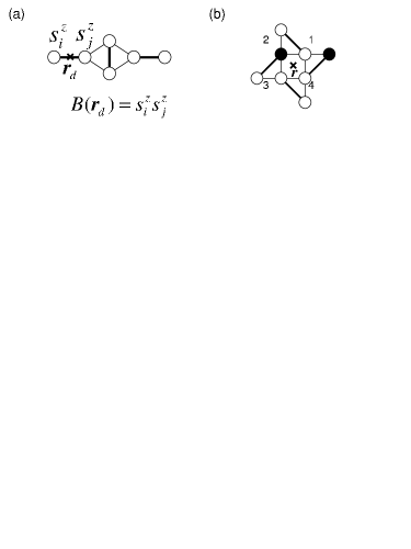
Figure 6: (a) A bond spin operator. The bond spin operator $B$ is defined by inner product of pair spins on each diagonal bond (bold line) and $B_{st}$ is the staggered magnetization of $B$. The bold black and gray lines indicate the sign of the factor $f({\bf r}_{d})$. (b) Definition of sublattice.

First, we show the results of the finite-temperature transition in the Ising limit ($\Delta_{\perp}=0$). The Monte Carlo simulations up to $L=120$ were performed at $J^{\prime}/J=0.3$ and $J_{4}/J=-(1/\sqrt{2})^{3}\times J^{\prime}/J\sim-0.106$. Fig. 7 (a) displays the temperature dependence of the correlation ratio of the bare spins at $(x,y)=(L_{x}/2,0)$ and $(L_{x}/3,0)$ for different system sizes. The curves cross at the critical temperature $T_{c}\sim 0.09050(10)$, reflecting the size invariance of the correlation ratio at the critical temperature. The spin fluctuations freeze at this temperature. Fig. 7 (b) and (c) show the temperature dependence of the Binder ratios $R_{B}$ for $B_{st}$ and $R_{S}$ for $m_{x}^{c}$, respectively. The system size dependence of both Binder ratios disappears at the same critical temperature. The crossing of the curves for $R_{B}$ and $R_{S}$ also indicates that the $C_{4}$ symmetry breaks down to the trivial group at $T_{c}\sim 0.09050(10)$. The obtained results suggest that the transition belongs to the universality class of the four-state Potts model. This is confirmed by finite-size scaling analysis. For the fourth order cumulant of $B_{st}$ and $m_{x}^{c}$, we assume the scaling forms $U_{R}=F(tL^{1/\nu})$ and $U_{S}=F(tL^{1/\nu})$, where $F$ is a scaling function and $U_{R}$ and $U_{S}$ denote the fourth order cumulant of $B_{st}$ and $m_{x}^{c}$, respectively. For the static structure factor of the bond spins, $S_{B}L^{2\beta/\nu}=F(tL^{1/\nu})$ is assumed, where $S_{B}=\sum_{{\bf r}_{d}}B({\bf r}_{d})\exp{[i\pi(r_{x}+r_{y})]}$. In the analysis, the critical exponents and the critical temperature are fixed at $\nu=2/3$, $\beta=1/12$Domb and $T_{c}=0.09050(10)$, The results are shown in Fig. 8. The excellent data collapse confirms that the transition in the Ising limit belongs to the universality class of the four state Potts model.

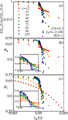
Figure 7: (color online) Temperature dependence of the correlation ratio at $J_{4}/J\sim-0.106$ in the Ising limit case. (a) Correlation ratio of the bare spin correlation. (b) The Binder ratio $R_{B}$ of the bond-spin operator $R_{st}$. (c) The Binder ratio $R_{S}$ of $m_{x}^{c}$.

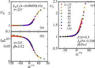
Figure 8: (color online) Finite-size scaling analysis for $U_{R}$, $S_{B}$, and $U_{S}$ in the Ising limit case. (a) and (c) are the results for the fourth-order cumulant $U_{R}$ and $U_{S}$. (b) Scaling analysis for the static structure factor $S_{B}$ of bond spins.

Next, we show the results of the quantum spin model with $\Delta_{\perp}=0.25$. We performed computations up to $L=84$. Fig. 9 shows the temperature dependence of the same order parameters as those defined in the above. The obtained results clearly indicate that the transition is a two-step process.

The curves for $R_{B}$ cross at $k_{B}T_{c1}/J=0.0815(3)$. This means that Néel order of the bond spins $B$ is realized for $T<T_{c1}$. Since a quotient group $C_{4}/C_{2}$, which is isomorphic to the group $C_{2}$, breaks down at $T_{c1}$, it is naively expected that the transition belongs to the two-dimensional Ising model universality class. Accordingly we performed finite-size scaling analysis assuming the scaling form $U_{R}=F(tL^{1/\nu})$ and $\nu=1$. We emphasize here that the data collapse shown in Fig. 9 (c) and (d) was obtained without any adjustable parameter, confirming that the transition at $T_{c1}$ indeed belongs to the two-dimensional Ising universality class.

Fig. 9 (b) shows the temperature dependence of the Binder ratio $R_{S}$ for $m_{x}^{c}$, and it provides an evidence of the other phase transition. The curves for $R_{S}$ for different system sizes intersect at $k_{B}T_{c2}/J=0.0580(5)$ and the difference $T_{c1}-T_{c2}$ is approximately $0.03J$, slightly larger than the previously obtained valueSuzuki . The universality class of the phase transition at $T_{c2}$ should be the same as that of the two-dimensional Ising model because the remaining symmetry $C_{2}$ is also isomorphic to $Z_{2}$. This is confirmed by the finite-size scaling results presented in Fig. 9 (e) where we have used the same scaling function and critical exponent as for $R_{B}$, viz. $U_{S}=F(tL^{1/\nu})$ and $\nu=1$. Consequently, we conclude that there $exists$ an intermediate phase with $C_{2}$-rotation symmetry phase that can be characterized by the bond Néel order accompanying the internal antiferromagnetic bare-spin fluctuation. The schematic spin configuration in this $C_{2}$-rotation symmetry phase is shown in Fig. 2 (e).

If the antiferromagnetic fluctuation on the bond $J$ is relevant to the stabilization of the intermediate phase, the temperature range of the $C_{2}$-rotation symmetric phase expands upon increasing $\Delta_{\perp}$. In Fig. 10, $\Delta_{\perp}$ dependence of the critical temperatures is presented for fixed $J^{\prime}/J=0.3$, $H/J=1$ and $J_{4}/J=-(1/\sqrt{2})^{3}\times J^{\prime}/J\sim-0.106$. The results show that the critical temperature associated with the breaking of the $180\,^{\circ}$ rotational symmetry shifts to the lower temperature as $\Delta_{\perp}$ increases. This suggests that the dimerization of antiparallel spin on the diagonal bonds plays a key role in the transition. As discussed in the followings, the phase diagram is qualitatively understood from a comparison with that of the generalized chiral four-state clock model.

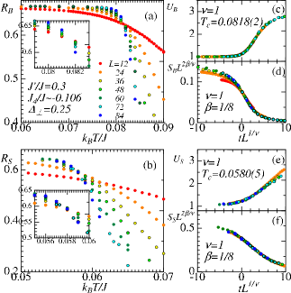
Figure 9: (color online) Finite-temperature transition to the $1/2$ plateau phase. (a) and (b) are temperature dependence of the Binder ratio of $R_{B}$ and $R_{S}$, respectively. (c) and (d) are the results of the finite-size scaling analysis for fourth-order cumulant $U_{R}$ of staggered magnetization $B_{st}$ and the static structure factor $S_{B}$ of bond spins. (e) and (f) correspond to (c) and (d) for $m_{x}^{c}$. In (f), the static structure factor of $m_{x}^{c}$ is calculated from $S_{S}=\sum_{\bf r}m_{x}^{c}({\bf r})\exp[-i(\pi r_{x}+\pi r_{y})]$

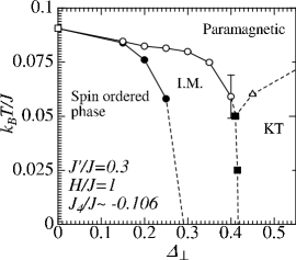
Figure 10: Phase diagram at $J^{\prime}/J=0.3$ and $J_{4}/J=-(1/\sqrt{2})^{3}\sim-0.106$. I.M. in the phase diagram means the $C_{2}$-rotational symmetric phase. Schismatic spin configurations in the spin ordered phase and I.M. are shown in Fig. 2 (d) and (e), respectively. Open and solid circles indicate the second order transition with the two-dimensional Ising universality, and an open square is that with the four-state Potts universality. An open triangle is the Kosterslitz-Thouless transition. All lines are guide to the eyes.

IV Comparison to a classical model

In the previous section, we have investigated the finite-temperature phase transition to the $m=1/2$ plateau phase for the classical and quantum spin models. Since the symmetry of both models is same and the finite-temperature phase transition is focused on, it is expected that the schematic phase diagram should be the same. However, the results obtained are different from this expectation. In order to understand the discrepancy, we consider the generalized chiral four-state clock model. As we show below, this simplified classical model captures the characteristics of phase diagram for the original model.

We begin by introducing eight-spin unit clusters (windmill clusters) in the $m=1/2$ plateau state as shown in Fig. 6(b). In this phase, a down spin occupies one of four sites on a plaquette without the diagonal bond and up spins occupy the remaining three sites. If a down spin occupies the site labeled by ‘2’ in Fig. 6(b), the nearest down spin prefers to locate at the third-neighbor distance from it as long as the ferromagnetic $J_{4}$ coupling. This indicates that the down spins in the $m=1/2$ plateau state occupies the same edge of diagonal bond connecting each plaquette. Since the ferromagnetic $J_{4}$ coupling is essential for stabilizing the $m=1/2$ plateau state (as discussed in Sec. II), it is reasonable to describe the $m=1/2$ plateau state by an arrangement of such clusters. This description becomes exact in the limit $|J_{4}/J|\gg 1$ and $\Delta_{\perp}=0$.

In the Ising limit $\Delta_{\perp}=0$, the spin configuration in the $m=1/2$ plateau state can be expressed by the arrangement of the windmill clusters shown in Fig. 11 (a). There are four kinds of clusters corresponding to the $90\,^{\circ}$-rotation symmetry breaking in the $m=1/2$ plateau. We assign clock spins pointing at an angle to each clusters. Here we ignore clusters having $m\neq 1/2$ for simplicity. Thus we obtain the simplified classical Hamiltonian that can be regarded as the generalized four-state clock model on a square lattice with the nearest and next-nearest neighbor interactions,

$${\mathcal{H}}_{sim} = {\mathcal{H}}_{\rm N.N.}+{\mathcal{H}}_{\rm N.N.N}$$

$${\mathcal{H}}_{\rm N.N.} = \sum_{i}\mathcal{J}_{x}(\theta_{i,j},\theta_{i+1,j})+\sum_{j}\mathcal{J}_{y}(\theta_{i,j},\theta_{i,j+1})$$

$${\mathcal{H}}_{\rm N.N.N} = \sum_{i}\mathcal{J^{\prime}}_{x}(\theta_{i,j},\theta_{i+1,j+1})+\sum_{j}\mathcal{J^{\prime}}_{y}(\theta_{i,j},\theta_{i-1,j+1}),$$ (6)

where $\theta_{i,j}$ denotes an angle of clock spins and takes $0,\pi/2,\pi$, or $3\pi/2$. The value of $\theta_{i,j}$ denotes the position of a down spin in the windmill clusters (see Fig. 11 (a)). ${\mathcal{J}}_{x}$ and ${\mathcal{J}}_{y}$ are interactions between two clock spins, and their values are listed in Table I. The interactions, ${\mathcal{J}}_{x}$ and ${\mathcal{J}}_{y}$, are calculated from the sums of coupling energy between spins located in different clusters. When $\Delta_{\perp}=0$, the values, A, B, C, and D, in ${\mathcal{J}}_{x}$ and ${\mathcal{J}}_{y}$ (see Table I) are evaluated as A=4$J_{4}$, B=2$J^{\prime}$, C=0, D=4$J^{\prime}$, respectively. The resulting classical Hamiltonian retains $C_{4}$ rotational symmetry conditionally: the system requires a lattice rotation when a global angle shift of all clock spins is executed. Such requirement arises from the geometric characteristics of the SSL. Since the symmetry of the Hamiltonian ${\mathcal{H}}_{\rm N.N.}$ is lower than that of ${\mathcal{H}}_{\rm N.N.N.}$, we focus on the critical properties of ${\mathcal{H}}_{\rm N.N.}$ in the followings.

Table 1: Coupling constants of the simplified classical Hamiltonian. Note that (A, B, C, D)=($4J_{4}$,$2J^{\prime}$,$0$, $4J^{\prime}$) corresponds to the parameter set we have treated in the section III. Upper (lower) side tables are matrices of the nearest neighbor (next-nearest neighbor) interaction.

${\mathcal{J}}_{x}(\theta_{i,j},\theta_{i+1,j})$
$\theta_{i,j}\backslash\theta_{i^{\prime},j^{\prime}}$	0	$\pi/2$	$\pi$	$3\pi/2$
0	A	B	C	B
$\pi/2$	B	A	B	D
$\pi$	C	B	A	B
$3\pi/2$	B	-D	B	A

${\mathcal{J}}_{y}(\theta_{i,j},\theta_{i,j+1})$
$\theta_{i,j}\backslash\theta_{i^{\prime},j^{\prime}}$	0	$\pi/2$	$\pi$	$3\pi/2$
0	A	B	D	B
$\pi/2$	B	A	B	C
$\pi$	-D	B	A	B
$3\pi/2$	B	C	B	A

${\mathcal{J}}^{\prime}_{x}(\theta_{i,j},\theta_{i+1,j+1})$
$\theta_{i,j}\backslash\theta_{i^{\prime},j^{\prime}}$	0	$\pi/2$	$\pi$	$3\pi/2$
0	A	C	A	C
$\pi/2$	C	A	C	-A
$\pi$	A	C	A	C
$3\pi/2$	C	-A	C	A

${\mathcal{J}}^{\prime}_{y}(\theta_{i,j}\backslash\theta_{i-1,j+1})$
$\theta_{i,j}\backslash\theta_{i^{\prime},j^{\prime}}$	0	$\pi/2$	$\pi$	$3\pi/2$
0	A	C	-A	C
$\pi/2$	C	A	C	A
$\pi$	-A	C	A	C
$3\pi/2$	C	A	C	A

The simplified Hamiltonian ${\mathcal{H}}_{\rm N.N.}$ is identical to the conventional four-state Potts model in the limit B=C=D=0. Therefore, it is trivial that the finite-temperature phase transition at this point is a single second-order transition belonging to the four-state Potts universality. However, the universality class becomes nontrivial, when B$\neq$D$\neq$0. Performing Monte Carlo simulations, we numerically investigated the finite-temperature transition of the classical Hamiltonian ${\mathcal{H}}_{\rm N.N.}$ with D=2B and A=-4 up to $L=72$. We summarize the obtained critical temperatures in Fig. 12 (a). These critical temperatures were estimated from the finite-size scaling analysis for the Binder ratio and correlation ratio of the order parameters, $\langle\cos\theta\rangle$ and $\langle\cos 2\theta\rangle$.

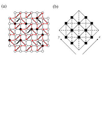
Figure 11: (a) Windmill clusters and clock spins in the simplified classical model (color online). A cluster is constructed by eight spins. Red dashed lines drawing windmills correspond to the clusters and arrows in the windmills denote angles of clock spins that represent states of the clusters. (b) Generalized four-state clock model on a square lattice. Solid squares correspond to each clusters described in (a). Solid (dashed) lines denote the nearest (next-nearest) neighbor interaction ${\mathcal{J}}_{x}$ and ${\mathcal{J}}_{y}$ (${\mathcal{J}}^{\prime}_{x}$ and ${\mathcal{J}}^{\prime}_{y}$).

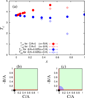
Figure 12: (color online) (a) Critical temperatures of the generalized four-state clock model when we fix at B/A=-0.05 and C/A=0. The higher and lower critical temperatures were calculated by the finite-size scaling analysis for the Binder ratio of $\langle\cos\theta\rangle$ and $\langle\cos 2\theta\rangle$, respectively. Red and blue symbols correspond to the cross sections on red solid and dashed lines drawn in (b) and (c), respectively. (b) and (c) are expected phase diagrams of the present clock model. In (b) and (c), an area painted by green indicates the region where the two-step phase transition with two-dimensional Ising universality takes place. A blue quarter circle in (c) means the area where the system undergoes a single phase transition.

In the following, we focus on the results when C/A=0 and B/A are varied (along the y-axis in Fig. 12 (b) and (c)). For C/A=0, the system undergoes a single second-order transition when the coupling ratio satisfies ${\rm B/A}>-0.075$. To identify the universality class, we performed finite-size scaling analysis and present the results in Fig. 13. (The scaling forms assumed here are the same as those shown in the previous section.) In the analysis, we estimated $T_{c}$ from the crossing of the curves for the correlation ratio, $\Gamma_{\cos n\theta}(L/2)/\Gamma_{\cos n\theta}(L/4)$, for different system sizes, where $\Gamma_{\cos n\theta}(r)=\langle\cos n\theta_{0,0}\cdot\cos n\theta_{r,r}\rangle$ and $n=1,2$. For ${\rm B/A}>-0.07$, excellent data collapse is obtained with $\nu=2/3$ and $\beta=1/12$. This strongly suggests that the transition belongs to universality class of the four-state Potts modelDomb . For ${\rm B/A}<-0.075$, the critical exponent increases from $\nu=2/3$ to $\nu=1$ with the fixed ratio $\beta/\nu\sim 1/8$ as B/A decreases. For ${\rm B/A}\leq-0.5$, we confirm a clear evidence of two-step phase transition with $\nu=1$ at both critical temperatures. Therefore, the critical properties for ${\rm B/A}\leq-0.5$ belong to the two-dimensional Ising universality class.

Next we discuss the results when the parameters are varied along the dashed lines in Fig. 12 (b) and (c), where B/A=-0.05 and $0\leq{\rm C/A}\leq 1$. For ${\rm C/A>0.25}$, the system clearly undergoes a two-step phase transition with both transitions belonging to the two-dimensional Ising universality class. Fig. 14 presents the results of the finite-size scaling analysis at B/A=-0.05 and C/A=0.5. When the two-step phase transition takes place, the $90\,^{\circ}$ rotation symmetry breaks at the higher critical temperature and the $180\,^{\circ}$ rotation symmetry survives in the intermediate phase. The lower critical temperature decreases as the difference between A and C decreases. For ${\rm C/A>1}$, the system seems to undergo a single phase transition and the $180\,^{\circ}$ rotation symmetry survives for any finite temperature.

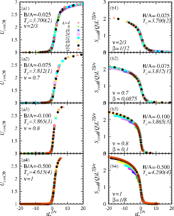
Figure 13: (color online) (a1) - (a4) ((b1) - (b4)) are the results of finite size scaling analysis for the fourth-order cumulant of $\langle\cos 2\theta\rangle$ (the static structure factor of $\cos\theta$) when C/A=0. In these analysis, we estimated all critical temperatures from crossing points of the correlation ratios $\langle\Gamma_{\cos\theta}(L/2)\rangle/\langle\Gamma_{\cos\theta}(L/4)\rangle$ and $\langle\Gamma_{\cos 2\theta}(L/2)\rangle/\langle\Gamma_{\cos 2\theta}(L/4)\rangle$. The data collapse in (a1) and (b1) ((a4) and (b4)) was obtained by using the fixed critical exponents $\nu=2/3$ and $\beta=1/12$ ($\nu=1$ and $\beta=1/8$). The critical exponents in (a2), (b2), (a3), and (b3) were estimated to minimize the discrepancies among data.

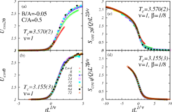
Figure 14: (color online) Finite size scaling analysis for fourth order cumulant of the order parameters $\langle\cos 2\theta\rangle$ (a) and $\langle\cos\theta\rangle$ (b) at B/A=-0.1 and C/A=0.5. (c) and (d) are the same analysis for the structure factor of each order parameter. In these analysis, each critical temperature is estimated from a cross of the correlation ratios $\langle 2\cos\theta_{L/2,0}\rangle/\langle\cos 2\theta_{L/4,0}\rangle$ and $\langle\cos\theta_{L/2,0}\rangle/\langle\cos\theta_{L/4,0}\rangle$. All results are obtained by using the fixed critical exponents $\nu=1$ and $\beta=1/8$.

The obtained results allow us to consider two scenarios of the phase diagram for the present four-state clock model. One is that the system shows a single phase transition only at B=C=0 and the two-step phase transition takes place for ${\rm B/A}<0$ and ${\rm C/A}>0$ as shown in Fig. 12 (b). The other is that there exists a region having the four-state Potts universality class around ${\rm B/A}={\rm C/A}=0$, denoted by the area in Fig. 12 (c). The critical exponents may show a crossover behavior at the boundary of the area. Further studies of the critical behavior of the extended four-state clock model are currently underway.

We compare the phase diagrams shown in Fig. 10 and Fig. 12 here. The topology of the phase diagram for the simplified classical model is the same as that of the Ising-like XXZ model on the SSL. In both models, the region of the intermediate phase, where only the $90\,^{\circ}$ rotational symmetry is broken, shrinks rapidly as the system approaches the four-state-Potts universality point. When we consider the quantum effects in the original Hamiltonian (3), fluctuation of antiferromagnetic spin pairs on the diagonal bond is enhanced when $\Delta_{\perp}$ increases. Then, the sublattice magnetization of antiparallel spin pair closes to zero. In the case, where the antiparallel spin pair becomes a classical or quantum-triplet dimer with $S^{z}=0$, the clock spins pointing towards $\theta=0$ and $\pi$ (or $\pi/2$ and $3\pi/2$) direction can not be distinguished from each other. Such dimerization effect is captured as a reduction in the difference between A and C. Consequently, the lower transition temperature $T_{c2}$ associated with the $180\,^{\circ}$ rotational symmetry breaking shifts toward $T=0$ as $\Delta_{\perp}$ increases.

By considering the parameter set associated with the Ising limit of the original Hamiltonian, we can estimate a parameter set of ${\mathcal{H}}_{\rm N.N.}$ as A$\approx 4J_{4}$, B$\approx 2J^{\prime}$, C$\approx 0$, and D$\approx 4J^{\prime}$. For $J^{\prime}/J=0.3$ and $J_{4}/J\sim-0.106$, ${\mathcal{H}}_{\rm N.N.}$ shows a single phase transition with the critical exponent $\nu\sim 1$, in clear disagreement with that of the original model. This is because we ignored the effect of the next-nearest neighbor couplings and the other states excluded from the four states treated here. A more quantitative estimation of the parameter set (A,B,C,D) is required by adding such effects for a quantitative mapping of the original Hamiltonian over the entire parameter range, but this is beyond the scope of this paper.

V ${\rm TmB_{4}}$

Finally, we discuss the magnetization properties of ${\rm TmB_{4}}$. The $m=1/2$ plateau state is observed for $H_{c1}\sim$1.9[T]$<H<$$H_{c2}\sim$3.6[T] at 2[K]TmB4_1 . The coupling ratio $J^{\prime}/J\sim 1$ and a strong Ising anisotropy $\Delta_{\perp}<<1$ are expected from the crystal structure of ${\rm TmB_{4}}$ and specific heat measurementsSiemensmeyer . These experimental results help us estimate the other parameters for the present model. We obtain $J_{3}/J\sim 0.1182$ and $J_{4}/J<-0.25$ at $J^{\prime}/J=1$ from the local energy estimation in the Ising limit. The magnetization curves at fixed $J_{3}/J=0.1182$, $J_{4}/J=-0.251$, $J^{\prime}/J=1$ and $k_{B}T/J=0.15$ are shown in Fig. 15 (a). It is found that the magnetization jumps appear at $H_{c1}/J\sim 1.4$ and $H_{c2}/J\sim 2.65$ not only in the Ising limit but also for $\Delta>0$. From these critical fields, we roughly estimate $(H_{c2}-H_{c1})$/$H_{c1}\sim 0.9$. This value is in good agreement with the experimental value. Therefore our estimation for the coupling ratio is quantitatively consistent with the critical fields of the magnetization jumps observed in ${\rm TmB_{4}}$.

The $m\sim 1/8$ plateau observed in the experiments TmB4_2 ; TmB4_4 appears to depend on the history of the system; $m\sim 1/8$ was observed around $H\sim 1.8$[T], when the fields were decreased from the saturation fields, whereas the magnetization remained vanishingly small around $H\sim 1.8$[T] during the upsweep. In other words, a hysteresis loop was observed around $H\sim 1.8$[T]. The inset of Fig. 15 (a) is the magnetization curves at $k_{B}T/J=0.05$ when we perform field sweeps. We started with the Néel state (the fully-polarized state) and increased (decreased) the applied field from $H/J=0$ ($H/J=3$). A hysteresis behavior similar to the experiments can be observed in short-time simulations. Although the Monte Carlo dynamics is not directly comparable to the real dynamics, this similarity is suggestive. The magnetization curves in the inset suggest a presence of shoulder around $m=1/8$ for $0.9<H/J<1.2$. In this field region, we have confirmed the existence of a mixed state comprised of the Néel order and domain walls constructed of fully-polarized spin chains from the snapshot of spin configuration. The period of the domain walls is fluctuating and the average of the period changes continuously as the field decreases. Thus, the shoulder around $m=1/8$ seems to be a transient process in successive plateaus having the magnetization $0<m<1/2$. Since the magnetization value of the shoulder shifts to the lower magnetization value as the system size increases, it seems to be smeared out in the thermodynamic limit. More quantitative discussion of the $m=$1/8 shoulder is desirable via comparison with the other experimental observations.

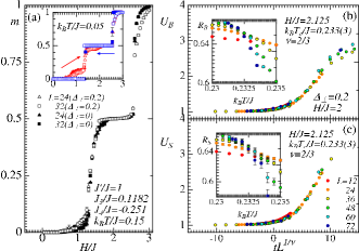
Figure 15: (color online) (a) Magnetization curves at $J^{\prime}/J=1$, $J_{3}/J=0.1182$ $J_{4}/J=-0.251$. Red solid (open) symbols represent the results of the Ising limit case (the quantum spin model case) when they have been obtained by the field sweeps from $H/J=3$ and the slow cooling. Blue ones are the results of the field sweeps from $H/J=0$. Inset of (a) is the results of short time Monte Carlo calculations when the field sweep is performed. (b) and (c) show a finite-size scaling analysis for the fourth-order cumulant of $R_{B}$ and $R_{S}$, respectively.

We comment the finite-temperature transition to the $m=1/2$ plateau phase. Using the above parameters, we have studied it for the Ising spin model and the quantum spin model numerically. Fig. 15 (b) and (c) are the results of the scaling analysis, when the quantum spin model is considered. The results indicate that a single second-order transition takes place and the critical exponent equals $\nu\sim 2/3$. The obtained results indicate that the critical property of the finite-temperature transition to the $m=1/2$ plateau phase can be explained by that of the four-state Potts model. This critical behavior was also confirmed in the Ising limit case. Therefore, if our estimation for the coupling constants is correct, we expect the experimentally observed critical exponents in ${\rm TmB_{4}}$ to belong to the four-state Potts universality class.

The $m=1/2$ plateau has been observed in the other SSL compound ${\rm ErB_{4}}$ErB4 . The magnetic moments of ${\rm ErB_{4}}$ are derived from ${\rm Er^{3+}}$ ions and the magnitude equals $J=15/2$. In this compound, the strong Ising anisotropy perpendicular to the SSL plains has been suggested. When we focus on the magnetic properties at a very low temperature, the effective Hamiltonian of the magnetic properties can be also described by the present model in the Ising limit. Therefore we believe that our results help understand the magnetic order of the $m=1/2$ plateau observed in ${\rm ErB_{4}}$.

VI Summary

In summary, we have studied the magnetic properties of a model of interacting spins with Ising-like exchange anisotropy and longer range interactions on the SSL that captures the low-temperature magnetic properties of the rare-earth tetraboride, ${\rm TmB_{4}}$. We have focused on the finite-temperature transition to the $m=1/2$ plateau phase and investigated the universality class of the transition. In the Ising limit, the system shows a single second-order transition. The critical behavior is well explained by that of the four-state Potts model. When there exists quantum exchange interactions, it has been confirmed that there is the two-step phase transition with an intervening intermediate phase. Both the transitions are belonging to the two-dimensional Ising universality class. From the finite-size scaling analysis, we have ascertained that the intermediate phase can be characterized by the ”$180\,^{\circ}$-rotation symmetric” state retaining $\pi$-rotation symmetry on individual triplets with $m_{z}=0$. Since the symmetry of the quantum spin model is the same as that of the classical spin version, it is naively expected that the critical behavior of both models will also be the same. However, the obtained results have indicated that the phase diagrams for the finite-temperature transition are different. To understand the critical behavior of both the models, we have proposed the simplified classical model, namely the generalized four-state chiral clock model. By performing the Monte Carlo computations for the simplified classical model, we have found that the universality class at the critical temperatures and the topology of the phase diagram are in agreement with those of the original models on the SSL. Finally, we have studied the magnetic properties of ${\rm TmB_{4}}$. From the Ising limit analysis, we have estimated the parameters that can explain (qualitatively) the magnetization curves observed in experiments. From the short-time Monte Carlo simulations, we have suggested that the $m\sim 1/8$ plateau seems to be a metastable state. We have also investigated the finite-temperature transition to the $m=1/2$ plateau state. If our estimation for the coupling constants is correct, measurements of the critical exponents belonging to the universality class of the four-state Potts model are expected in experiment.

References

- (1) S. Onoda and Y. Tanaka, Phys. Rev. Lett. 105, 047201 (2010).
- (2) Z. Y. Meng, T. C. Lang, S. Wessel, F. F. Assaad, and A. Muramatsu, Nature 464 , 847 (2010).
- (3) S.E. Sebastian, N. Harrison, P. Sengupta, C. D. Batista, S. Francoual, E. Palm, T. Murphy, H. A. Dabkowska, and B. D. Gaulin, PNAS 105, 20157 (2008).
- (4) B. S. Shastry and B. Sutherland, Physica B 108, 1069 (1981).
- (5) H. Kageyama, K. Oknizuka, Y. Ueda, N. V. Mushnikov, T. Goto, K. Yoshimura, A. Kosuge, J. Phys. Soc. Jpn. 67, 4304 (1998).
- (6) H. Kageyama, K. Yoshimura, R. Stern, N. V. Mushnikov, K. Onizuka, M. Kato, K. Kosuge, C. P. Slichter, T. Goto, and Y. Ueda, Phys. Rev. Lett. 82, 3168 (1999).
- (7) M. Takigawa, T. Waki, M. Horvatic, and C. Berthier, J. Phys. Soc. Jpn. 79, 11005 (2010).
- (8) S. Miyahara and K. Ueda, J. Phys.: Condens. Matt. 15, R327 (2003).
- (9) A. Koga and N. Kawakami, Phys, Rev, Lett, 84, 4461 (2000).
- (10) A. Lauchli, S. Wessel, and M. Sigrist, Phys. Rev. B 66, 014401 (2002).
- (11) T. Momoi and K. Totsuka, Phys. Rev. B 62, 15067 (2000).
- (12) S. Yoshii, T. Yamamoto, M. Hagiwara, T. Takeuchi, A. Shigekawa, S. Michimura, F. Iga, T. Takabatake, and K. Kindo, J. Magn. Magn. Mater. 310, 1282-1284 (2007).
- (13) S. Michimura, A. Shigekawa, F. Iga, M. Sera, T. Takabatake, K. Ohyama, and Y. Okabe, Physica B 378-380, 596-597 (2006).
- (14) S. Yoshii, T. Yamamoto, M. Hagiwara, A. Shigekawa, S.Michimura, F. Iga, T. Takabatake, and K. Kindo, J. Phys.: Conf. Ser. 51, 59-62 (2006).
- (15) K. Siemensmeyer, E. Wylf, H.-J. Mikeska, K. Flachbart, S. Gabáni, S. Maa, P. Priputen, A. Evdokimova, and N. Shitsevalova, arXiv:0712.1537 (2007).
- (16) F. Iga, A. Shigekawa, Y. Hasegawa, S. Michimura, T. Takabatake, S. Yoshii, T. Yamamoto, M. Hagiwara, K. Kindo, J. Magn. Magn. Mater, 310, e443-e445 (2007).
- (17) S. Gabáni, S. Matas, P. Priputen, K. Flachbart, K. Siemensmeyer, E. Wulf, A. Evdokimova, and N. Shitsevalova, Acta. Phys. Pol. A 116, 227 (2008).
- (18) K. Siemensmeyer, E. Wulf, H.-J. Mikeska, K. Flachbart, S. Gabáni, S. Matas, P. Priputen, A. Efdokimova, and N. Shitsevalova, Phys. Rev. Lett. 101, 177201 (2008).
- (19) Z. Y. Meng and S. Wessel, Phys. Rev. B 78, 224416 (2008).
- (20) F. Liu and S. Sachdev, arXiv:0904.3018.
- (21) M.-C. Chang and M.-F. Yang, Phys. Rev. B 79, 104411 (2009).
- (22) T. Suzuki, Y. Tomita, and N. Kawashima, Phys. Rev. B 80, 180405(R) (2009).
- (23) Y. Kato and N. Kawashima, Phys. Rev. E 79, 021104 (2009).
- (24) J. Dorier, K. P. Schmidt, and F. Mila, Phys. Rev. Lett. 101, 250402 (2008).
- (25) K. Fukui and S. Todo, J. Comp. Phys. 28, 2629 (2009).
- (26) B. Niehuis, in Phase transition and Critical Phenomena, edited by C. Domb and J. L. Lebowitz (Adademic Press, New York, 1987), Vol. 11.
- (27) The energy gains of the plateau, plateau and the fully polarized state are , , and .