Transaction fees and optimal rebalancing
in the growth-optimal portfolio

Abstract

The growth-optimal portfolio optimization strategy pioneered by Kelly is based on constant portfolio rebalancing which makes it sensitive to transaction fees. We examine the effect of fees on an example of a risky asset with a binary return distribution and show that the fees may give rise to an optimal period of portfolio rebalancing. The optimal period is found analytically in the case of lognormal returns. This result is consequently generalized and numerically verified for broad return distributions and returns generated by a GARCH process. Finally we study the case when investment is rebalanced only partially and show that this strategy can improve the investment long-term growth rate more than optimization of the rebalancing period.
Keywords: growth-optimal portfolio, Kelly game, transaction fees, lognormal distribution.

¹ Physics Department, Renmin University, 100872 Beijing, PR China
² Complexity Research Center, USST, 200093 Shanghai, PR China
³ Physics Department, University of Fribourg, 1700 Fribourg, Switzerland
⁴ Lab of Information Economy and Internet Research, University of Electronic Science
⁴ and Technology, 610054 Chengdu, PR China

1 Introduction

Portfolio optimization is one of the main topics in quantitative finance. The aim is to maximize investment return while simultaneously minimizing its risk (see [1, 2] for a review of the modern portfolio theory). Pioneering works on this problem were mainly focused on the Mean-Variance approach [3] where the portfolio variance is minimized under the constraint of a fixed expected return value. A different approach has been put forward by Kelly [4] who focused on repeated investments and proposed to maximize the long-term growth rate of the investor’s capital. This so-called growth-optimal or Kelly portfolio has been shown to be optimal according to various criteria [5] and generalized in different ways. For example, the question of diversification and constant rebalancing among a certain number of uncorrelated stocks was investigated in [6]. In [7], the authors showed that there is a close connection between the Mean-Variance approach and the Kelly portfolio and that in many cases, the Kelly-optimal portfolio includes only a small fraction of the available profitable assets. When investing in games without specified levels of risk and reward, the Kelly criterion can be merged with Bayesian statistical learning as in, for example, [8, 9], yielding generalized results for the optimal investment fractions. Stochastic portfolio theory [10] is also a descendant of Kelly’s approach by utilizing on a logarithmic representation of price processes.

Application of Kelly’s optimization process to real stock prices was studied in [11] with the conclusion that non-trivial investment (i.e., investing only a part of one’s wealth) occurs rarely. This is related to the general notion that Kelly’s portfolio is very aggressive and investment outcomes are sensitive to errors in estimates of assets’ properties. Modifications such as fractional Kelly strategies [12] and controlled downturns [13] have been consequently proposed to make the resulting portfolios more secure (these modifications can be of particular importance for risky assets [14]). Optimization in the long-term can even explain the emergence of cooperation in environments where outcomes of the participants are of multiplicative nature [15]. An interested reader is referred to [14, 16] for a comprehensive introduction to the Kelly portfolio.

Kelly’s optimization scheme is based on the long-term prospects of the investor and requires continual rebalancing of the portfolio which ensures that the investment fraction is kept constant. This rebalancing represents the key advantage of the Kelly portfolio over the simple buy-and-hold strategy. On the other hand, when non-zero transaction costs are imposed, resulting investment performance may deteriorate considerably (for an example of how the transaction costs influence real traders and their decisions see [17]). In this paper we intend to study the effect of non-zero transaction costs on the Kelly portfolio. We study the situation where portfolio is rebalanced less often (intermittent rebalancing). Our key quantity of interest is the optimal rebalancing period which minimizes the negative effects of transaction fees while maintaining the positive effects of frequent rebalancing.

Another reason for intermittent rebalancing is that the distribution of returns may differ from one turn to another. We approach this problem by postulating a risky asset which evolves on two different time scales and its return distribution hence regularly varies in time. This setting allows us to study the interplay between the time scales and portfolio rebalancing. Considering a risky asset with a lognormal return distribution allows us to obtain an analytical form for the optimal rebalancing period. This result is further generalized to other stationary return distributions with finite variance and used to explain some observations made for binary return distributions. Our numerical simulations show that similar behavior can be observed even for returns generated by the standard $\textrm{GARCH}(1,1)$ process where consecutive returns are not independent. Finally, we briefly study partial rebalancing where the investor transfers only a certain part of the required amount between cash and the risky asset. We show that this strategy can enhance the long-term growth rate more than intermittent rebalancing.

2 Basic Model

Consider a situation where an investor with an initial wealth $W_{0}$ is allowed to repeatedly invest a fraction $f$ of the current wealth to a risky asset while keeping the rest in cash. We assume that the asset price $x(t)$ undergoes a multiplicative stochastic process

$$x(t+1)=\Big{\{}\begin{aligned} x(t)(1+r_{1})&\qquad\text{with probability $\tfrac{1}{2}+P_{1}$},\\ x(t)(1-r_{1})&\qquad\text{with probability $\tfrac{1}{2}-P_{1}$}\end{aligned}$$ (1)

at discrete time steps $t$ ($t=1,2,3,\dots$) and $x(1)=1$. Here $r_{1}$ is a positive parameter ($0<r_{1}\leq 1$) representing the rate of gain or loss of the investment, $\tfrac{1}{2}+P_{1}$ is the “winning” probability and $P_{1}\in(0,\tfrac{1}{2}]$ (when $P_{1}<0$, the asset is not profitable and it is advisable to refrain from investment); it is assumed that they are both constant and known to the investor. This “symmetric” setting can be easily generalized by assuming distinct rates of gain/loss (e.g., $r_{1}$ and $r_{1}^{\prime}$) as well as their probabilities (e.g., $P_{1}$ and $P_{1}^{\prime}$). To keep the notation simple and to limit the number of parameters to minimum, we treat only the symmetric case here. By setting $r_{1}=1$, one recovers the original Kelly game studied in [4].

Since asset’s properties do not change with time and investor’s wealth follows a multiplicative process, the investment fraction set by a rational investor has to be the same in all time steps. Investor’s wealth after $N$ investment turns is therefore

$$W_{N}=W_{0}(1+fr_{1})^{w}(1-fr_{1})^{N-w}$$ (2)

where $w$ and $N-w$ is the number of “winning” and “loosing” turns, respectively. Now we can introduce a so-called exponential growth rate of investor’s wealth, $G$, which is defined by the relation $W_{N}=W_{0}\exp[GN]$. Its limit value has the form

$$G:=\lim_{N\to\infty}\frac{1}{N}\ln\frac{W_{N}}{W_{0}}.$$ (3)

One can easily show that for the given model parameters this converges to the unique value

$$G(f)=(\tfrac{1}{2}+P_{1})\ln(1+fr_{1})+(\tfrac{1}{2}-P_{1})\ln(1-fr_{1}).$$ (4)

In the case of a general risky asset with return distribution $\varrho(r)$, this formula generalizes to the form

$$G(f)=\big{\langle}\ln(1+fr)\big{\rangle}_{\varrho}$$ (5)

where the average is over the return distribution $\varrho(r)$. The long-term profitability of the risky asset can be measured by the average return per time step, $R$. By definition, $W_{N}=W_{0}(1+R_{N})^{N}$ and $R=\lim_{N\to\infty}R_{N}$. Using Eq. (3), $R$ can be expressed in terms of $G$ simply as

$$R=\exp(G)-1.$$ (6)

Both $G$ and $R$ are functions of the asset parameters $r_{1},P_{1}$ and of the investment fraction $f$.

According to the Kelly portfolio strategy [4], for a long-term investment it is best to maximize the growth rate $G$ (or, equivalently, the long-term return $R$)—this strategy is therefore sometimes referred to as the growth-optimal investment strategy. Starting from Eq. (4), simple computation yields the optimal investment fraction

$$f_{1}^{*}=2P_{1}/r_{1}.$$ (7)

Increasing the value of $P_{1}$ enhances the asset’s profitability and leads to an increased optimal investment fraction. On the other hand, increasing $r_{1}$ enhances the asset’s expected return (when $P_{1}>0$) but it also increases the magnitude of losses; overall it leads to a decreased value of $f^{*}$. When $P_{1}>r_{1}$, we obtain $f^{*}>1$ which means that the investor is advised to borrow additional money and invest them in the risky asset too. When $P_{1}<0$ (the asset is not profitable), $f^{*}<0$ which corresponds to the so-called short selling. For simplicity we assume that both borrowing and short selling are forbidden and hence $f\in[0;1]$.

3 Transaction fees and intermittent portfolio rebalancing

The requirement of keeping the investment fraction $f$ constant implies that the investor needs to constantly rebalance the portfolio: after a “winning” turn, some part of wealth has to be moved from the asset to cash and after a “loosing” turn, some additional wealth has to be invested in the asset. This constant portfolio rebalancing may require payment of substantial transaction fees. The question is, how the fees affect the portfolio optimization process. In particular, we are interested whether there are situations where the investor fares better with intermittent rebalancing which is sub-optimal from the point of view of the Kelly strategy but requires fewer money transfers and hence lowers the transaction fees.

3.1 Transaction fees

We assume that for any wealth $X$ transferred from or to the risky asset, a transaction fee $\alpha\lvert X\rvert$ must be paid ($\alpha>0$; the absolute value reflects the fact that transaction fees are paid regardless of the direction of the transfer). How to include $\alpha$ in the derivation of the optimal investment fraction presented above? Given that the portfolio is properly balanced at a certain moment, the total amount invested in the risky asset is $fW$. If the realized return from the risky asset is $r$, the total wealth changes to $W(1+fr)$ and the invested amount changes to $fW(1+r)$. If $r>0$, wealth $X>0$ needs to be transferred from the risky asset to cash to keep the portfolio balanced. The resulting total wealth is then $W(1+fr)-\alpha X$ and the invested amount is $fW(1+r)-X$. To achieve the investment fraction $f$, it must hold that

$$f\big{[}W(1+fr)-\alpha X\big{]}=fW(1+r)-X.$$ (8)

From this formula it follows immediately that the total transferred volume is $X_{r>0}=Wrf(1-f)/(1-\alpha f)$. As expected, no transfer is needed when $f=0$ or $f=1$; transaction fees have no effect on portfolio optimization in these two cases. When $r<0$, the transferred volume can be derived in a similar way and has the form $X_{r<0}=Wrf(1-f)/(1-\alpha(1-f))$. Now we know the wealth lost to transaction fees which allows us to write investor’s wealth after $N$ time steps

$$W_{N}=W_{0}\left[1+fr_{1}-\frac{\alpha r_{1}f(1-f)}{1-\alpha f}\right]^{w}\left[1-fr_{1}-\frac{\alpha r_{1}f(1-f)}{1-\alpha(1-f)}\right]^{N-w}.$$ (9)

This is a generalization of Eq. (2) for the case with transaction fees.

It is straightforward to use Eq. (9) to obtain the exponential growth rate $G(f)$ and maximize it to get the optimal investment fraction. Since the resulting quadratic equation has complicated coefficients and provides little insights to the behavior of the system, we introduce an approximate approach which will be of great importance in later more complicated cases. We expand $\mathrm{d}G/\mathrm{d}f$ in terms of $\alpha,P_{1},r_{1}$ and keep only terms up to order $\alpha$ (this is motivated by the fact that the transaction fee coefficient $\alpha$ is nowadays usually small in practice). Assuming that $P_{1}$ and $r_{1}$ are sufficiently small, we neglect terms that are of the order higher than $P_{1}^{2}$, $P_{1}r_{1}$, or $r_{1}^{2}$. The resulting optimal fraction then has the simple form

$$f_{1}^{*}(\alpha)=\frac{2P_{1}-\alpha}{r_{1}-2\alpha}.$$ (10)

Fig. 1 illustrates the dependency of this result on both $P_{1}$ and $\alpha$. Naturally, in the limit $\alpha\to 0$ we recover the fee-free result $f_{1}^{*}=2P_{1}/r_{1}$. Interestingly, transaction fees may both decrease and increase the optimal investment fraction (in comparison with the value corresponding to $\alpha=0$). On the other hand, the average return is always reduced by transaction fees.

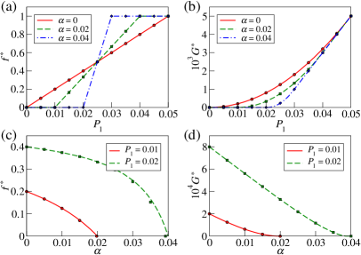
Figure 1: The influence of transaction fees on the optimal investment: the dependency on $P_{1}$ for $r_{1},\alpha$ fixed (a,b) and the dependency on $\alpha$ for $r_{1},P_{1}$ fixed (c,d) $r_{1}=10\%$ in all cases. Analytical and numerical results are shown as lines and symbols, respectively.

Using Eq. (10), one can solve the equation $f_{1}^{*}(\alpha)=0$ to obtain a lower bound for $P_{1}$ at which the asset becomes profitable, $P_{1}^{\mathrm{low}}=\alpha/2$. As expected, $P_{1}^{\mathrm{low}}$ is greater than the fee-free lower bound which means that transaction fees decrease the asset’s profitability. Similarly, one can solve the equation $f_{1}^{*}(\alpha)=1$ to obtain an upper bound for $P_{1}$ at which the investor is advised to invest all wealth in the asset, $P_{2}^{\mathrm{up}}=(r_{1}-\alpha)/2$ which is less than the threshold $r_{1}/2$ valid for $\alpha=0$. We can conclude that transaction fees narrow the region where non-trivial optimal investment fractions ($0<f_{1}^{*}<1$) realize (this effect is well visible in Fig. 1a). Another point of view is that transaction fees modify the optimal investment fraction $f^{*}$ so that the transferred amounts (which are approximately proportional to $(1-f)f$) are lowered. Transaction fees are in this sense similar to friction in mechanics which also both attenuates motion and leads to dissipation of energy (in the case of transaction fees we face dissipation of wealth).

3.2 Intermittent portfolio rebalancing

While in the original Kelly game the investor should rebalance the portfolio as often as possible (i.e., after each time step), in the presence of transaction fees it may be profitable to rebalance the portfolio less often. Our goal is to solve the intermittent portfolio optimization problem first without and then with transaction fees. Denoting the investor’s rebalancing period as $T$, the probability of “winning” in $w$ steps out of $T$ is binomial and reads

$$B_{1}(w|T)=\binom{T}{w}(\tfrac{1}{2}+P_{1})^{w}(\tfrac{1}{2}-P_{1})^{T-w}.$$

Since the asset’s return in $T$ time steps can be written as

$$r_{w}=(1+r_{1})^{w}(1-r_{1})^{T-w}-1,$$

we know the return distribution and Eq. (5) gives the exponential growth rate

$$G(f)=\sum_{w=0}^{T}B_{1}(w|T)\ln\big{[}1+fr_{w}\big{]}$$ (11)

where substitution $T=1$ recovers $G(f)$ given by Eq. (4). Using Eq. (9), it is easy to generalize this result to the case with both intermittent rebalancing and transaction fees, yielding

$$G(f)=\sum_{w=0}^{T}B_{1}(w|T)\ln\bigg{[}1+fr_{w}-\frac{\alpha f(1-f)\lvert r_{w}\rvert}{1-\alpha\chi(f,r_{w})}\bigg{]}$$ (12)

where $\chi(f,r_{w})=f$ if $r_{w}>0$ and $\chi(f,r_{w})=1-f$ otherwise.

Eq. (12) cannot be maximized analytically in general and one has to resort to numerical techniques. When $T=2$, the approach that we developed to derive Eq. (10) yields

$$f_{2}^{*}(\alpha)=\frac{8P_{1}-\alpha(2+r_{1})}{4r_{1}-2\alpha(2+r_{1})}.$$ (13)

Notice that in the limit $\alpha\to 0$, this result is identical with the optimal portfolio fraction for rebalancing after each turn which is a direct consequence of assuming that $P_{1}$ and $r_{1}$ are small. Numerical tests show that Eq. (13) is reasonably precise for $\alpha,P_{1}\ll 1$.

Solution of the optimization problem for $T=2$ allows us to ask what transaction fee $\alpha_{x}$ makes rebalancing every other turn as profitable (in terms of the exponential growth rate $G$) as rebalancing in every turn. Using Eqs. (7), (11), (13) one can show that when $\alpha=0$, the difference of the optimal growth rates per turn is

$$G_{1}^{*}(0)-\tfrac{1}{2}G_{2}^{*}(0)=P_{1}^{2}(r_{1}-2P_{1})^{2}$$

where we neglected fifth and higher powers of $P_{1}$ and $r_{1}$ in the result. (The factor $1/2$ at $G_{2}^{*}(0)$ converts the exponential growth rate in two-turn basis to the growth rate per turn.) Assuming that $P_{1},r_{1},\alpha$ are small, it is also possible to find that the growth rates depend on $\alpha$ as

$$G_{1}^{*}(\alpha) =G_{1}^{*}(0)-\frac{2P_{1}}{r_{1}}(r_{1}-2P_{1})\alpha+O(\alpha^{2}),$$

$$G_{2}^{*}(\alpha) =G_{2}^{*}(0)-\frac{P_{1}}{r_{1}}(r_{1}-2P_{1})(2+r_{1})\alpha+O(\alpha^{2}).$$

Both growth rates are for $P_{1}=0$ and $P_{1}=r_{1}/2$ independent of $\alpha$. This is not surprising: in those cases is $f^{*}=0$ or $f^{*}=1$ and hence no rebalancing is necessary and the optimal exponential growth rate is unaffected by transaction fees. Combining the obtained results together, the equality $G_{1}^{*}(\alpha)=G_{2}^{*}(\alpha)/2$ can be solved with respect to $\alpha$, leading to

$$\alpha_{x}=2r_{1}P_{1}\frac{r_{1}-2P_{1}}{2-r_{1}}$$ (14)

which represents the magnitude of $\alpha$ for which rebalancing in every turn and in every other turn are equally profitable. As shown in Fig. 2, this formula is very accurate even for moderate values of parameters $P_{1},r_{1}$. It is instructive to note that the threshold fee value $\alpha_{x}$ is small for weakly profitable assets ($P_{1}$ small) and in particular for assets with small return in one step ($r_{1}$ small).

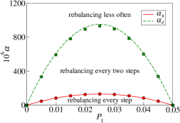
Figure 2: Intermittent rebalancing: numerical and approximate analytical values (shown as symbols and lines, respectively) of $\alpha_{x}$ and $\alpha_{z}$ for $r_{1}=10\%$.

In a very similar way it is possible to study the transaction fee at which rebalancing every two turns is as profitable as rebalancing every three turns. Interestingly, the resulting value $\alpha_{y}=2P_{1}(r_{1}-2P_{1})$ is for $r_{1}<1$ greater than $\alpha_{x}$ (by the factor of $(2-r_{1})/r_{1}$). This means that rebalancing every three turns is quite ineffective and hence it is meaningful to ask what $\alpha_{z}$ makes rebalancing every two and four turns equally profitable. The corresponding value

$$\alpha_{z}=16P_{1}r_{1}\frac{r_{1}-2P_{1}}{2+r_{1}}$$ (15)

is greater than $\alpha_{x}$ for $\alpha<9/14$ and it is smaller than $\alpha_{y}$ for $r_{1}<2/7$. This means that rebalancing every three turns is sub-optimal in the case of small investment returns: it is better to rebalance either more (for $\alpha>\alpha_{z}$) or less ($\alpha<\alpha_{z}$) often. As shown in Fig. 2, while precision of $\alpha_{z}$ is lower than that of $\alpha_{x}$, obtained values agree well with a purely numerical treatment of the problem.

When $r_{1},P_{1},\alpha$ are given, it is natural to ask what rebalancing period $T^{*}$ maximizes the exponential growth rate per turn. While this question cannot be answered analytically, it is straightforward to solve it numerically. Results are shown in Fig. 3 for various choices of $r_{1},P_{1}$. As can be seen, $T^{*}$ decreases with both $P_{1}$ and $r_{1}$. This agrees with the growth of the threshold values $\alpha_{x},\alpha_{z}$ with $P_{1}$ (until $P_{1}<r_{1}/4$) and $r_{1}$ (see Eqs. (14), (15)). When transaction fees are small, $T^{*}$ is proportional to $\alpha^{2/3}$—a behavior which will be explained in Sec. 4. When $\alpha\gtrsim 10^{-2}$, this scaling breaks down and $T^{*}$ grows even faster than linearly. Since this mode of behavior occurs only for exceedingly large transaction fees (note that $\alpha=1$ corresponds to confiscating all invested amount), we do not study it further.

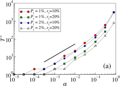
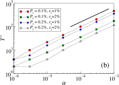
Figure 3: Optimal rebalancing periods $T^{*}$ vs $\alpha$ for different choices of $r_{1}$ and $P_{1}$; the indicative thick lines have slope $2/3$.

3.3 Risky assets with multiple time scales

Assets’ properties are in real life generally non-stationary. To analyze investment in an asset with time-varying properties, we propose a simple model where the price of the asset undergoes a stochastic binary process on two distinct time scales. In addition to the basic time scale $1$, we add a longer scale of length $T_{2}$. We assume that price of the asset undergoes a multiplicative dynamics given by Eq. (1) at all time steps and when $(t\mod T_{2})=0$, there is an additional return $\pm r_{2}$ with probabilities $\tfrac{1}{2}+P_{2}$ and $\tfrac{1}{2}-P_{2}$, respectively (as before, asset parameters are constrained to $0<r_{2}\leq 1$ and $0<P_{2}\leq 1/2$). This framework is a simple generalization of the original Kelly game to the case with non-stationary game properties and multiple time scales.

The simplest case is when the investor keeps the investment fraction $f$ constant and rebalances the investment every $T$ steps. Since price dynamics is still binary, we can parametrize the outcome by the number of “winning” turns on the basic time scale, $w_{1}$, and by the number of “winning” turns on the longer time scale, $w_{2}$. While $w_{1}$ is simply constrained to $0,\dots,T$, the upper bound for $w_{2}$ can be either $T\backslash T_{2}$ or $1+T\backslash T_{2}$ ($\%$ and $\backslash$ denote the modulus operator and integer division, respectively). Simple algebra shows that the odds of the two cases are $1-(T\%T_{2})/T_{2}$ and $(T\%T_{2})/T_{2}$, respectively, hence we can write the long-term exponential growth rate of the portfolio in the form

$$G= \big{(}1-\tfrac{T\%T_{2}}{T_{2}}\big{)}\sum_{w_{1}=0}^{T}\sum_{w_{2}=0}^{t}B_{1}(w_{1}|T)B_{2}(w_{2}|t)\ln\bigg{[}1+fr_{t}-\frac{\alpha f(1-f)\lvert r_{t}\rvert}{1-\alpha\chi(f,r_{t})}\bigg{]}+$$ (16)

$$+\tfrac{T\%T_{2}}{T_{2}}\sum_{w_{1}=0}^{T}\sum_{w_{2}=0}^{t+1}B_{1}(w_{1}|T)B_{2}(w_{2}|t+1)\ln\bigg{[}1+fr_{t+1}-\frac{\alpha f(1-f)\lvert r_{t+1}\rvert}{1-\alpha\chi(f,r_{t+1})}\bigg{]}$$

where $t:=T\backslash T_{2}$,

$$r_{t}=(1+r_{1})^{w_{1}}(1-r_{1})^{T-w_{1}}(1+r_{2})^{w_{2}}(1-r_{2})^{t-w_{2}}-1$$

is the compound return before transaction fees are applied and $B_{2}(w_{2}|t)$ is the binomial probability of $w_{2}$ wins in $t$ trials when the winning probability is $\tfrac{1}{2}+P_{2}$. Albeit principally simple, the described situation is out of scope of analytical optimization tools and hence we report only numerical results here. The most interesting behavior is obtained when the risky asset is profitable only on the longer time scale (that is, $P_{1}<0$ and $P_{2}>0$). The need to rebalance often (which is a principal property of the Kelly portfolio) then directly competes with the asset profitability on a longer time scale. An example of the resulting behavior is shown in Fig. 4 where irregularities corresponding to the longer time scale are visible on both $f^{*}(T)$ and $G^{*}(T)$. On the other hand, when $T\gg T_{2}$, the two time scales merge into average behavior of the risky asset and the irregularities are not visible anymore. We can conclude that the presence of multiple time scales is important only if portfolio rebalancing occurs in time intervals comparable to the longest time scale of asset’s returns.

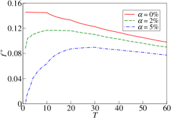
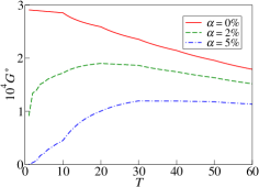
Figure 4: Optimal investment fraction and growth rate of the Kelly portfolio for an asset with price change on two time scales with $P_{1}=-0.01$, $r_{1}=0.05$, $P_{2}=0.05$, $R=0.5$, $T_{2}=10$.

4 Intermittent rebalancing for lognormal returns

Now we shall study portfolio optimization for a simple asset with lognormally distributed returns. We assume that the asset’s price $p_{i}(t)$ ($i=1,\dots,N$) undergoes an uncorrelated multiplicative random walk

$$p(t)=p(t-1)\mathrm{e}^{\eta(t)}$$

where random variable $\eta(t)$ is drawn from the Gaussian distribution with mean $m$ and variance $D$. Consequently, returns of the asset have the form

$$r(t):=\frac{p(t)}{p(t-1)}-1=\mathrm{e}^{\eta(t)}-1.$$

Using the same notation as above, the investor’s expected exponential growth rate has the form $G(f)=\langle\ln(1+fr)\rangle$ where the average is over different values of $\eta$. Written in detail, the previous expression reads

$$G(f)=\int_{-\infty}^{\infty}\mathrm{d}\eta\varrho(\eta)\ln\big{[}1+f(\mathrm{e}^{\eta}-1)\big{]}$$

where $\varrho(\eta)$ is the Gaussian probabilistic density of returns. With transaction fees, $G(f)$ generalizes to the form

$$G(f)=\int_{-\infty}^{\infty}\mathrm{d}\eta\varrho(\eta)\ln\big{[}1+f(\mathrm{e}^{\eta}-1)-\frac{\alpha f(1-f)\lvert\mathrm{e}^{\eta}-1\rvert}{1-\alpha\chi(f,\mathrm{e}^{\eta}-1)}\big{]}.$$ (17)

When $\alpha=0$, it is known (see [7]) that the optimal investment fraction has the approximate form

$$f_{0}^{*}(m,D)=\frac{1}{2}+\frac{m}{D}$$ (18)

which is valid when $m,D\ll 1$. Here $f_{0}^{*}=0$ for $m<-D/2$ and $f_{0}^{*}=1$ for $m>D/2$ (when $f$ is out of the range $[0,1]$, the investor has a non-zero probability of going bankrupted and hence the long-term growth rate is automatically zero [7]). In our following analysis we will hence assume that $m$ and $D$ are of the same order of smallness.

When $\alpha>0$, we search the optimal fraction in the form $f^{*}(\alpha)=f^{*}(0)+u$ where the correction $u$ is small when $\alpha$ is small. Since our goal is to find the highest order correction to $f^{*}$, we neglect the term $\alpha\chi(f,\mathrm{e}^{\eta}-1)$ in Eq. (17). The optimal investment fraction is the solution of $\partial G/\partial f=0$. By exchanging the order of derivation and integration we obtain

$$\frac{\partial G}{\partial f}=\int_{-\infty}^{0}\frac{(\mathrm{e}^{\eta}-1)(1+\alpha-2\alpha f)\varrho(\eta)\mathrm{d}\eta}{1+f(\mathrm{e}^{\eta}-1)[1+\alpha(1-f)]}+\int_{0}^{\infty}\frac{(\mathrm{e}^{\eta}-1)(1-\alpha+2\alpha f)\varrho(\eta)\mathrm{d}\eta}{1+f(\mathrm{e}^{\eta}-1)[1-\alpha(1-f)]}$$

where it was necessary to write two separate terms because of the absolute value $\lvert\mathrm{e}^{\eta}-1\rvert$ present in $G(f)$. We can now substitute $f=f_{0}^{*}+u$ where $f_{0}^{*}$ is the solution of $\partial G/\partial f=0$ for $\alpha=0$ (see Eq. (18) above). Assuming that both $\alpha$ and $u$ are small, the integrand of the first integral can be approximated as

$$\frac{(1+\alpha-2\alpha f_{0}^{*})x(\eta)}{1+(u+\alpha f_{0}^{*}(1-f_{0}^{*})x(\eta)}\approx x(\eta)\big{[}1+\alpha(1-2f_{0}^{*})-\big{(}u+\alpha f_{0}^{*}(1-f_{0}^{*})\big{)}x(\eta)\big{]}$$

where $x(\eta)=(\mathrm{e}^{\eta}-1)/(1+(\mathrm{e}^{\eta}-1)f_{0}^{*})$. The second integral can be manipulated in a similar way; by putting the results together we get

$$\frac{\partial G}{\partial f}=\int_{-\infty}^{\infty}\mathrm{d}\eta\varrho(\eta)\big{[}x(\eta)+\alpha(2f_{0}^{*}-1)\lvert x(\eta)\rvert-ux(\eta)^{2}\big{]}$$

which is equivalent to three separate integrals. The first one is zero by definition (we assume that $f_{0}^{*}$ is the solution for $\alpha=0$). For the second and third integral, we use $x(\eta)\approx\mathrm{e}^{\eta}-1$ (because $m,D\ll 1$ and hence $\eta$ is small) and $\varrho(\eta)\approx\exp[-\eta^{2}/(2D)]/\sqrt{2\pi D}$ (because $D\ll 1$ and $\lvert m\rvert\leq D/2$ and hence $\lvert m\rvert\ll\sqrt{D}$). While the integration results are complicated and involve the error function, for $D\ll 1$ we can simplify them further to finally obtain

$$\frac{\partial G}{\partial f}=\alpha(2f_{0}^{*}-1)D-u\sqrt{\pi D^{3}/2}.$$

Thus $u$ that maximizes $G$ (solution of $\partial G/\partial f=0$) has the form

$$u=\alpha m\sqrt{\frac{8}{\pi D^{3}}}$$

with the next contributing term of the order of $O(\sqrt{D})$. In combination with Eq. (18) we have

$$f^{*}(m,D,\alpha) =\frac{1}{2}+\frac{m}{D}+\alpha m\sqrt{\frac{8}{\pi D^{3}}},$$ (19)

$$G^{*}(m,D,\alpha) =G^{*}(m,D,0)-\alpha\bigg{(}\frac{1}{4}-\frac{m^{2}}{D^{2}}\bigg{)}\sqrt{\frac{2D}{\pi}}.$$

As shown in Fig. 5a, this agrees well with numerical results for $f^{*}$ (numerical results for $G^{*}$ are not shown).

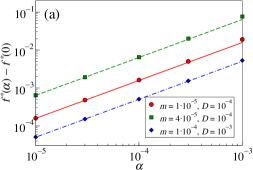
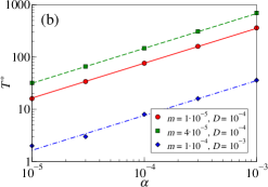
Figure 5: The dependency of the optimal investment fraction (a) and the optimal rebalancing period (b) on $\alpha$: numerical and analytical results are shown with symbols and lines, respectively.

When $\alpha=0$, by expanding $\ln[1+f(\mathrm{e}^{\eta}-1)]$ in Eq. (17) into a series of $f(\mathrm{e}^{\eta}-1)$ we get the following approximate expression for the optimal exponential growth rate

$$G^{*}(m,D)=\frac{D}{2}\bigg{(}\frac{1}{2}+\frac{m}{D}\bigg{)}^{2}-\frac{D^{2}}{4}\bigg{(}\frac{1}{4}-\frac{m^{2}}{D^{2}}\bigg{)}^{2}+O(D^{3}).$$

When the rebalancing period is $T$, the compound return of the asset is again lognormally distributed, this time with $\eta$ drawn from the Gaussian distribution with mean $Tm$ and variance $TD$ (here we take the advantage from the fact that the Gaussian distribution is stable). Using the above expression for $G^{*}(m,D)$ we can write the resulting optimal growth rate per time step as

$$G^{*}(m,D,T):=G^{*}(Tm,TD)/T\approx\frac{D}{2}\bigg{(}\frac{1}{2}+\frac{m}{D}\bigg{)}^{2}-\frac{TD^{2}}{4}\bigg{(}\frac{1}{4}-\frac{m^{2}}{D^{2}}\bigg{)}^{2}$$ (20)

which is a decreasing function of $T$ as expected. Combining this result with Eq. (19) produces a general dependency of the optimal growth rate on $T$ and $\alpha$. This dependency can be simply maximized with respect to $T$, yielding

$$T^{*}(m,D,\alpha)=\frac{\alpha^{2/3}}{D}\sqrt{\frac{8}{\pi}}\bigg{(}\frac{1}{4}-\frac{m^{2}}{D^{2}}\bigg{)}^{-2/3}$$ (21)

which is confirmed by comparison with numerical simulations in Fig. 5b (small irregularities visible for $D=10^{-3}$ are caused by true $T^{*}$ being an integer number). After multiplying Eq. (21) with $D$ we obtain an expression for $DT^{*}:=D^{*}$ which can be understood as an optimal variance of lognormally distributed returns. When $\alpha=0$, this optimal variance is zero, indicating that the investor should rebalance the portfolio continuously.

Results derived for the lognormal distribution of returns are of particular importance when intermittent rebalancing is considered. If we write the return at time $t$ as $r(t):=p(t)/p(t-1)-1=\mathrm{e}^{\varrho(t)}-1$ where values $\varrho(t)$ are drawn from a probabilistic distribution with finite mean and variance, the compound return over a period of $T$ turns is

$$r_{T}(t):=p(t)/p(t-T)-1=\exp\bigg{[}\sum_{u=0}^{T-1}\varrho(t-u)\bigg{]}-1.$$

According to the central limit theorem, if variables $\varrho(t)$ are independent and $T$ is large, the sum $\sum_{u=0}^{T-1}\varrho(t-u)$ is approximately normally distributed and hence compound return $r_{T}(t)$ follows a lognormal distribution when the rebalancing period $T$ is long. This immediately explains the scaling $T^{*}\sim\alpha^{2/3}$ which was found numerically for binary returns in Sec. 3.2. The same reasoning applies to any $\varrho(t)$ following a broad distribution with finite variance. As an example, we use returns $r(t)=\mathrm{e}^{\sigma\chi(t)}-1$ where $\chi(t)$ is Student’s distribution with two degrees of freedom (the tails of $\chi(t)$ then decay as $\chi^{-3}$, hence $\chi(t)$ has finite variance). Since Student’s distribution is not stable, the distribution of returns for an arbitrary rebalancing period $T$ does not have a closed form and one cannot attempt to find the optimal rebalancing period analytically. We employ numerical simulations in which the exponential growth rate is maximized with respect to the investment fraction $f$ over $10^{6}$ time steps for rebalancing periods in the range $1,\dots,100$. The resulting optimal growth rates $G^{*}(T)$ are averaged over $10^{3}$ independent realizations of returns and finally yield the optimal rebalancing period which is again roughly proportional to $\alpha^{2/3}$ (see Fig. 6a).

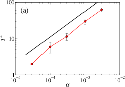
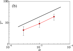
Figure 6: Optimal rebalancing period $T^{*}$ vs $\alpha$ for: (a) Student-based returns and (b) GARCH-based returns. The indicative dashed lines have slopes $0.70$ and $0.66$, respectively.

When aiming at even more realistic return distributions, it is a question whether $\alpha^{2/3}$-scaling holds for returns with some degree of dependence (memory). Since there are various central limit theorems for dependent variables [20, 21], one expects that when the dependence of returns is sufficiently weak, above-obtained results continue to hold. This is confirmed by our simulations with returns generated by a $\textrm{GARCH}(1,1)$ process [22, 23] with parameters $\alpha_{0}=10^{-5}$, $\alpha_{1}=0.2$, $\beta=0.7$ (these parameter values are similar to those inferred from S&P index data in [24]). The optimal rebalancing period—obtained by the same simulation approach as above for the Student-based returns—is again proportional to $\alpha^{2/3}$ (see Fig. 6b). This confirms that our main result is highly robust with respect to the nature of the return distribution. Detailed insights on the degree of dependence at which this scaling breaks down are however yet to come.

5 Partial rebalancing

So far we only considered mitigating the impact of transaction fees by intermittent rebalancing. There is another approach, which we call partial rebalancing, where only part of the required amount is transferred between cash and the asset. The transferred amount required to keep the investment fraction fixed is represented by $X$ in Eq. (8). If only part $\varepsilon$ of the required capital is transferred ($\varepsilon\in(0,1]$ is a rebalancing parameter), $1/\varepsilon$ steps would be needed to transfer the whole. Hence one can expect that partial rebalancing with $\varepsilon$ should be similar to intermittent rebalancing with period $T\approx 1/\varepsilon$. Since partial rebalancing is parametrized by a continuous parameter $\varepsilon$, it allows for smoother setting of the portfolio than intermittent rebalancing where the rebalancing period is integer.

When $\varepsilon<1$, the desired investment fraction is almost never achieved by partial rebalancing and the actual invested fraction fluctuates around it. (The smaller the value of $\varepsilon$, the larger the deviations; when $\varepsilon=1$, the standard rebalancing is recovered and the stake is always adjusted accurately.) Due to these irregularities, partial rebalancing is less accessible to analytical treatment and we present only numerical results here. As shown in Fig. 7, the optimal growth rates are achieved for $\varepsilon$ inside the range $(0,1]$. These rates outperform the optimal values obtained with intermittent rebalancing for both studied values of $\alpha$. If growth rate improvement is measured in respect to standard rebalancing (the same as obtained with $\varepsilon=1$), improvements obtained with partial rebalancing are 23% (for $\alpha=10^{-6}$) and 18% (for $\alpha=10^{-5}$) better than those obtained with intermittent rebalancing. As foreseen above, optimal values of $\varepsilon$ ($0.21$ and $0.06$, respectively) approximately correspond to the optimal periods of intermittent rebalancing ($4$ and $22$, respectively).

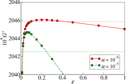
Figure 7: Optimal growth rate $G^{*}$ vs $\varepsilon$ for binary returns with $P_{1}=0.1\%$ and $r_{1}=1\%$. The two thick dotted lines show performance of intermittent rebalancing for $\alpha=10^{-6}$, $T=4$ (upper) and $\alpha=10^{-5}$, $T=22$ (lower), respectively.

6 Discussion

While transaction fees represent an important factor limiting investor’s profit, in finance literature they are often considered as uninteresting and neglected in order to keep the analysis simple and focused. However, money transfers required by active portfolio optimization strategies may be considerable and the effect of transaction fees significant. In this work we investigated this effect on the growth-optimal/Kelly portfolio in detail. To this end we studied a toy risky asset with a binary return distribution, an asset with time-depending return distribution, and more realistic assets with lognormal and fat-tailed return distributions. Our results show that transaction fees indeed have substantial impact on investment profitability, in particular when the average return of the risky asset is low. Their influence is greatest when the investment fraction is $1/2$. This is natural because the wealth volumes transferred in rebalancing are proportional to $f(1-f)$ and hence they are maximized at $f=1/2$.

We showed for various settings that when the transaction fee coefficient $\alpha$ is sufficiently high, for the investor it may be more profitable to adjust the portfolio less frequently and an optimal rebalancing period $T^{*}$ arises. In the case of a lognormal distribution of returns, the optimal optimal rebalancing period was analytically shown to be proportional to $\alpha^{2/3}$ for small $\alpha$. When $\alpha$ is small yet $T^{*}$ is sufficiently long for the central limit theorem to be an appropriate approximation, the optimal rebalancing period scales with $\alpha^{2/3}$ for any independent returns drawn from a distribution with finite mean and variance. Our numerical simulations confirm this for binary returns, returns based on Student’s distribution, and even for returns with memory modeled by a $\textrm{GARCH}(1,1)$ process where the requirement of independence is violated. We showed that a so-called partial rebalancing can also reduce the impact of transaction fees and hence improve the performance of the Kelly strategy.

Besides presented results, several research questions remain open. Firstly, while transaction fees are maximized by $f=1/2$ when investing in one asset, the situation gets more complicated when investment is distributed among several assets. That situation can be further generalized by assuming correlated asset returns. Secondly, through the paper we have assumed that parameters of the return distribution are known to the investor. Investment optimization hence only consists of choosing the right investment fraction. In real life, the return distribution itself is unknown and its estimation is part of the optimization process. Whether the presented results hold also this case is an open question. Finally, results for partial rebalancing presented in Sec. 5 show that this can be a superior approach to the Kelly optimization in presence of transaction fees. Observed similarity between optimal values of rebalancing parameters $T$ and $\varepsilon$ suggests that many of analytical results found here for intermittent rebalancing may hold also for partial rebalancing. Verification of this hypothesis remains as an important challenge for future research.

References

- [1] E. J. Elton, M. J. Gruber, S. J. Brown, W. N. Goetzmann, Modern Portfolio Theory and Investment Analysis, 7th edn., Wiley, 2006.
- [2] S. Zenios, W. Ziemba, Eds., Handbook of Asset and Liability Management, Volume 1, North-Holland, 2006.
- [3] H. M. Markowitz, The Journal of Finance 7, 77–91, 1952.
- [4] J. L. Kelly Jr., Bell System Technical Journal 35, 917–926, 1956.
- [5] H. M. Markowitz, The Journal of Finance 31, 1273–1286, 1976.
- [6] M. Marsili, S. Maslov, Y.-C. Zhang, Physica A 253, 403–418, 1998.
- [7] P. Laureti, M. Medo, Y. C. Zhang, Quantitative Finance 10, 689–697, 2010.
- [8] S. Browne, W. Whitt, Advances in Applied Probability 28, 1145–1176, 1996.
- [9] M. Medo, Y. M. Pis’mak, Y.-C. Zhang, Physica A 387, 6151–6158, 2008.
- [10] E. R. Fernholz, I. Karatzas, in Handbook of Numerical Analysis. Mathematical Modeling and Numerical Methods in Finance, A. Bensoussan, Ed., Elsevier, 89–168, 2009.
- [11] F. Slanina, Physica A 269, 554–563, 1999.
- [12] L. C. MacLean, W. T. Ziemba, G. Blazenko, Management Science 38, 1562–1585, 1992.
- [13] S. J. Grossman, Z. Zhou, Mathematical Finance 3, 241–276, 1993.
- [14] E. O. Thorp, in Handbook of Asset and Liability Management, Volume 1, S. Zenios and W. Ziemba, Eds., North-Holland, 385–428, 2006.
- [15] G. Yaari, S. Solomon, EPJ B 73, 625–632, 2010.
- [16] L. C. MacLean, W. T. Ziemba, in Handbook of Asset and Liability Management, Volume 1, S. Zenios and W. Ziemba, Eds., North-Holland, 429–474, 2006.
- [17] D. Morton de Lachapelle, D, Challet, New Journal of Physics 12, 075039, 2010.
- [18] R. C. Merton, Continuous-Time Finance, Blackwell, 1990.
- [19] S. Maslov, Y. C. Zhang, International Journal of Theoretical and Applied Finance 1, 377–387, 1998.
- [20] W. Hoeffding, H. Robbins, Duke Mathematical Journal 15, 773–80, 1948.
- [21] Yu.V. Prokhorov, V. Statulevicius, Eds., Limit Theorems of Probability Theory, Springer, 2000.
- [22] R. Engle, Journal of Economic Perspectives 15, 157–168, 2001.
- [23] S. J. Taylor, Modelling financial time series, 2nd Ed., World Scientific, 2008.
- [24] J.-C. Duan, Mathematical Finance 5, 13–32, 1995.