An Analysis of Transaction and Joint-patent Application Networks

Abstract

Many firms these days, forced by increasing international competition and an unstable economy, are opting to specialize rather than generalize as a way of maintaining their competitiveness. Consequently, they cannot rely solely on themselves, but must cooperate by combining their advantages.

To obtain the actual condition for this cooperation, a multi-layered network based on two different types of data was investigated. The first type was transaction data from Japanese firms. The network created from the data included 961,363 firms and 7,808,760 links. The second type of data were from joint-patent applications in Japan. The joint-patent application network included 54,197 nodes and 154,205 links. These two networks were merged into one network.

The first anaysis was based on input-output tables and three different tables were compared. The correlation coefficients between tables revealed that transactions were more strongly tied to joint-patent applications than the total amount of money. The total amount of money and transactions have few relationships and these are probably connected to joint-patent applications in different mechanisms. The second analysis was conducted based on the $\mbox{p}^{*}$ model. Choice, multiplicity, reciprocity, multi-reciprocity and transitivity configurations were evaluated. Multiplicity and reciprocity configurations were significant in all the analyzed industries. The results for multiplicity meant that transactions and joint-patent application links were closely related. Multi-reciprocity and transitivity configurations were significant in some of the analyzed industries. It was difficult to find any common characteristics in the industries. Bayesian networks were used in the third analysis. The learned structure revealed that if a transaction link between two firms is known, the categories of firms’ industries do not affect to the existence of a patent link.

1 Introduction

Many firms these days, forced by increasing international competition and an unstable economy, are opting to specialize rather than generalize as a way of maintaining their competitiveness. Consequently, they cannot rely solely on themselves, but must cooperate by combining their advantages. Although there are many ways for them to do this, in terms of competitiveness, the most important objective is creating novel products and services.

Intuitively, if firms create something new, they can sell more of their goods or services than they used to. The priority of this process is that cooperative research and development (R&D) comes first and transactions come second. However, firms cannot know what is innovative for their customers without selling any goods or services to them. Hence, it is natural for sellers to try to know what buyers want as much as possible. Consequently, the relationship between sellers and buyers develops and yields a new relationship as cooperative R&D. The priority in this process is that transactions come first and cooperative R&D comes second. Therefore, if we focus on the relationships between cooperative R&D and transactions, it is difficult to determine which relationship is built first. Since firms have to strategically cooperate more than ever, pursuing this question has become increasingly important. This question can be rephrased as “seeds and needs,” i.e., do seeds precede needs, or do needs precede seeds?

Based on the above, this paper investigates the relationship between cooperative R&D and transactions. The author acquired data that included exhaustive transactions and joint-patent applications made by Japanese firms. Based on the data, this paper discusses three different analyses.

The first is based on input-output tables. Input-output tables and their analyses were first developed by Leontief [1] and he used a matrix representation of the economy of some actors to predict the effect of changes in one industry on others and by others (consumers, government, and foreign suppliers.) However, the effect by others has not been considered in this paper. The input-output tables are used to analyze economics, and more concretely, the total amount of money flowing between industries. The present author created other types of matrices based on transactions (number of relationships between firms, not the total amount of money) and cooperative R&D. By comparing matrices, he discusses the relevance of cooperative R&D and other economic activities. The most important point is that this analysis is conducted on industries that are aggregates of firms and this is a basis for the second analysis.

The second analysis is conducted based on configurations of networks whose nodes are firms and links are transactions and cooperative R&D. Actors in matrices are industries and the relationships are investigated in the first analysis. However, actors are firms in the second analysis and more complicated structures between them are investigated. In the analysis, the present author uses the $\mbox{p}^{*}$ model [2] (this has recently been called the exponential random graph (ERG) model.) This method reveals whether a network includes significant configurations (some specific patterns or motifs) or not.

Bayesian networks are used in the third analysis. The Bayesian networks are completely different from the networks mentioned in this paper thus far and they are methods of finding causality from data. The Bayesian networks were first proposed by Pearl [3]. One of the objectives of this paper is to investigate which link (transactions or cooperative R&D) is created first. This means that we have to establish the causality between relationships. If one tends to be created first, that is evidence of causality.

The rest of this paper is organized as follows. Section 2 presents the data used in this paper. Section 3 explains the preparation of the input-output tables as the analysis. Section 4 explains the $\mbox{p}^{*}$ model for the second analysis, and Section 5 explains Bayesian networks for the third analysis. Section 6 concludes this paper.

2 Data

This paper explains the two different types of data that were used. The first type was transaction data from Japanese firms provided by Tokyo Shoko Research (a Japanese investigation firm). The data included 961,363 firms and 7,808,760 transactions that took place between them in 2005. The current author created a network from the data and the it had firms as nodes, and transactions as links. A link had a direction and a direction meant the flow of money. There is a degree distribution in Figure 1 that explains the whole structural characteristics. The horizontal axis indicates the degree and the vertical axis indicates the rank counted from the highest degree. We can see that the graph can be roughly fitted with a line except for the low degree; therefore, it does not have a peak like p normal distribution.

Figure 1: Degree distribution by rank in transaction network. Horizontal axis indicates degree and vertical axis indicates rank counted from highest degree.

The other data are joint-patent applications. These data were provided by Koukai Tokkyo Kouhou (publication issued by the Japanese Patent Office.) The data included 5,570,786 patents. The objective of this paper is to investigate the relationships between transactions and cooperative R&D and these patent data are used to identify cooperative R&D activity. Although cooperative R&D involves a wide variety of activities, patents are one of the most decisive items of evidence for cooperative R&D. A patent mainly has information on new findings and also has other information about the people or organizations that published the patent. This paper uses applicants that are in charge of patent applications. Most of the applicants are firms and this paper only treats firms. Therefore, applicants that are firms need to be distinguished from other types of applicants. As firms have a coorporate status in their names, this can be used to distinguish them. A patent possibly has more than one firm that are applicants, and that can be regarded as evidence of cooperative R&D activity. Hence, the network for joint-patent applications is composed of applicants as nodes, and joint-patent applications as links. If more than two nodes are involved in a patent, those nodes are connected in the manner of a complete graph. The joint-patent application network includes 54,197 nodes and 154,205 links between the firms. The links do not have a direction. The degree distribution is plotted in Figure 2 in the same way as in Figure 1. The horizontal axis indicates the degree and the vertical axis indicates the rank counted from the highest degree.

Inoue et al. recently studied the joint-patent application network [4]. Their study included an investigation into the existence of a power law in the degree distribution of the network. The least-squares method is generally used for verification, and the inclination (the power index) in the power-law distribution is estimated. However, this approach has two critical flaws. The first is that people cannot determine whether the distribution really follows a power law or not. The inclination can be estimated for any kind of distribution with this method. The second flaw is that people cannot determine which part of the distribution follows a power law. Consequently, we have the method created by Clauset, et al. [5] that combines maximum-likelihood fitting methods with goodness-of-fit tests based on the Kolmogorov-Smirnov statistic. If the probabilistic distribution of degree follows a power law, the equation for a discrete case can be expressed by

$$p(x)=\frac{x^{-\alpha}}{\zeta(\alpha,x_{\mbox{min}})},$$

where

$$\zeta(\alpha,x_{\mbox{min}})=\sum^{\infty}_{n=0}(n+x_{\mbox{min}})^{-\alpha},$$

Here, $x_{\mbox{min}}$ is the lower bound and $\alpha$ is the scaling parameter. $x_{\mbox{min}}$ is necessary because $p(x)$ diverges at $x=0$. The equation for the cumulative distribution is defined as

$$P(x)=\frac{\zeta(\alpha,x)}{\zeta(\alpha,x_{\mbox{min}})}.$$

As a result, the network for joint-patent applications is scale-free and $\alpha$ is 2.03 at $x_{\mbox{min}}=7$.

Figure 2: Degree distribution by rank in joint-patent application network. Horizontal axis indicates degree and the vertical axis indicates rank counted from highest degree.

The two networks for transactions and joint-patent applications are different. However, these two networks have firms and they can therefore be merged into one network that has firms as nodes, and transactions and joint-patent applications as links. These links should be distinguished; hence, the network includes two different types of links. The network has 975,607 nodes and this number is less than the sum of the number of nodes in the networks. This is because there are identical firms. The names and addresses of firms are used to identify them. Many nodes are duplicated if only names are used. If both are used, no duplication occurs and each node can be uniquely distinguished. The network is called a multi-layered network in this paper.

3 Input-output tables

The first analysis is based on input-output tables that were developed by Leontief [1]. An industry buys primary material or fuel, fabricates products from them, and sells these to other industries. Input-output tables list how many goods and services are produced and sold between industries. These tables are expressed by matrices. These matrices are very useful for calculating how much production increases in industries when some industry has exceptional needs. Japanese input-output tables are well known for their accuracy. The original input-output table included non-industrial actors (consumers, government, and foreign suppliers), but these have been omitted from this paper.

This paper’s objective is to discuss the relationships in transactions and joint-patent applications between firms. Input-output tables, on the other hand, handle the relationships between industries. Needless to say, industries are different from firms and they are aggregates of firms. The objective of this section is to explain the macroscopic trend in the relationships between firms.

Table 1 is a pedagogic example of an input-output table. This table is for “electrical machinery” and “information and communication machinery” industries. The rows mean output industries and the columns mean input industries. Therefore, 354 billion Japanese yen passed from the electrical machinery industry to the information and communication machinery industry. As we can see from the table the original input-output table provides flows for the total amount of money between industries. The matrix for the table was called $\mathbf{M_{a}}$.

The data for the input-output tables were published by the Japanese Statistics Bureau, and the Director-General for the Policy Planning and Statistical Research and Training Institute. There are many input-output tables and this paper uses tables from major consolidated industries . The number of major consolidated industries is 34. All of the industries are shown in Table 2 and 3.

However, we can create the matrices based on the number of transactions between firms, not the total amount of money or the number of joint-patent applications. By comparing three different matrices we can discuss the relevance between them. The author made two new 34 times 34 matrices. The matrix for the transation table is called $\mathbf{M_{t}}$, and the joint-patent application table is called $\mathbf{M_{p}}$. Figure 3 shows the difference between three matrices. The schematic at left is for a situation where money is flowing from an electrical machinery industry to an information and communication machinery industry ($\mathbf{M_{a}}$). Three hundred fifty four billion yen was assigned to the element of the matrix that corresponds to this pair. The upper right schematic is for a situation situation where money is flowing from an electrical machinery industry to an information and communication machinery industry. However, the value of the matrix is the number of transactions conducted by firms between industries ($\mathbf{M_{t}}$). The lower right figure is for a situation where firms have jointly applied for patents in an electrical machinery industry and those in an information and communication machinery industry ($\mathbf{M_{p}}$).

Figure 4 is a scatter plot for $\mathbf{M_{a}}$ and $\mathbf{M_{p}}$. Let $x$ represents the value for the horizontal axis and $y$ be that for the vertical axis. Then, each position on the plots corresponds to

$$(x,y)=(\mathbf{M_{a}}_{ij},\mathbf{M_{p}}_{ij}).$$

This means a plot corresponds to elements that have the same position in $\mathbf{M_{a}}$ and $\mathbf{M_{p}}$. Figure 5 is a scatter plot for $\mathbf{M_{t}}$ and $\mathbf{M_{p}}$ and Figure 6 is a scatter plot for $\mathbf{M_{t}}$ and $\mathbf{M_{a}}$.

Table 1: Pedagogic example of input-output tables. Numbers are flows for total amount of money. Money flows from industries in rows to ones in columns.

	Electrical machinery	Information and communication
		machinery
Electrical machinery	1,938 billion yen	354 billion yen
Information and communication machinery	2 billion yen	422 billion yen

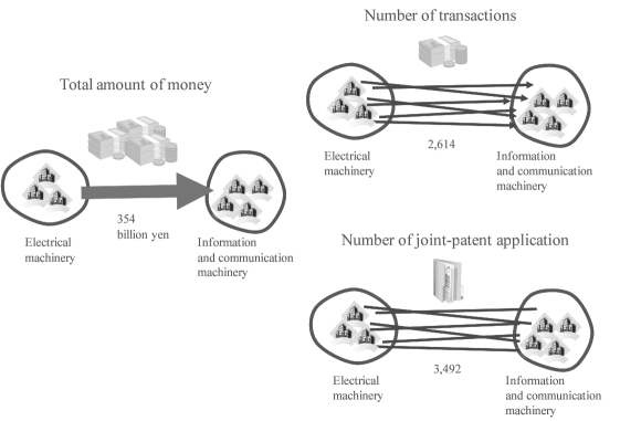
Figure 3: Difference between three matrices. These figures are examples and indicate how value of each matrix element is determined.

Figure 4: Scatter plot for $\mathbf{M_{a}}$ and $\mathbf{M_{p}}$. Each plot corresponds to elements that have same position in $\mathbf{M_{a}}$ and $\mathbf{M_{p}}$. Correlation coefficient is 0.31.

Figure 5: Scatter plot for $\mathbf{M_{t}}$ and $\mathbf{M_{p}}$. Correlation coefficient is 0.45.

Figure 6: Scatter plot for $\mathbf{M_{t}}$ and $\mathbf{M_{a}}$. Correlation coefficient is 0.05.

These figures are similar. However, the Pearson’s correlation coefficients for the scatter plots are 0.31 ($\mathbf{M_{a}}$ and $\mathbf{M_{p}}$), 0.45 ($\mathbf{M_{t}}$ and $\mathbf{M_{p}}$) and 0.05 ($\mathbf{M_{t}}$ and $\mathbf{M_{a}}$). The objective of this paper is to discuss the relationships in transactions and joint-patent applications between firms and the results reveal that either the total amount of money or transactions are strongly related to the number of joint-patent applications. The correlation coefficients indicate transactions are more strongly tied to joint-patent applications than the total amount of money. Since joint-patent applications represent the intensity of scientific and technological connections between industries, this means that the total amount of money can be used to track scientific and technological connections to some degree, but transactions are more preferable to reach the objective. The correlation coefficient for $\mathbf{M_{t}}$ and $\mathbf{M_{a}}$ is important and 0.05 means the total amount of money and transactions have few relationships and these are probably connected to joint-patent applications in different mechanisms.

4 $\mbox{P}^{*}$ model

The previous section explained that transactions are probably a better approach to understanding the relationships to joint-patent applications than the total amount of money at the industry level. This section presents the results and discusses configurations for the networks. The number of transactions and joint-patent applications were counted for industries in the previous section but this section returns the units to firms.

In the analysis, the current author uses the $\mbox{p}^{*}$ model [2] (this has recently been called the exponential random graph (ERG) model.) This method reveals whether a network includes significant configurations (some specific patterns or motifs) or not. To explain the $\mbox{p}^{*}$ model, this paper uses a dependence graph model [6].

First, dependence graphs are explained. They are graphs whose nodes are the links in some network. Figure 7 outlines an example of a dependence graph. The closed circles at the bottom represent the nodes in an existing network and the open circles at the top represent the nodes corresponding to the links in the lower network. The links between nodes in a dependence graph means there is a relationship between the links in an existing network. Since a dependence graph indicates what kinds of configurations there are in networks, the $\mbox{p}^{*}$ model can be understood by using this. The example in Figure 7 shows an existing network only has one type of link. Since this paper treats transaction and joint-patent application networks, dependence graphs include and distinguish between the two types of links.

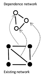
Figure 7: Example of dependence graph. Node in dependence graph corresponds to link in actual networks.

It is assumed in the $\mbox{p}^{*}$ model that a network is one entity where nodes are fixed and links are probabilistically created. Network $x$ is a notation whose links are determined in given nodes. The probability of $x$ in the model defined as

$$P(x)=\kappa^{-1}\mbox{exp}(\sum_{A\subseteq N_{D}}\lambda_{A}z_{A}(x)),$$ (1)

where $\kappa=\sum_{x}\mbox{exp}(\sum_{A\subseteq N_{D}}\lambda_{A}z_{A}(x))$, and this is a normalized constant. $A$ is a sub-class of nodes, and $N_{D}$ represents the nodes from the dependence graph. $x_{ijm}$ is the link from node $i$ to $j$ in network $m$ and $z_{A}(x)=\prod_{x_{ijm}\in A}x_{ijm}$. Network $m$ is a layer of networks. $\lambda_{A}$ is a coefficient. The essence of the $\mbox{p}^{*}$ model is to find $\lambda_{A}$ so that $P(x)$ is maximized.

There are many redundant configurations in Equation (1) of the $\mbox{p}^{*}$ model corresponding to $\lambda$. We have to reduce the number of $\lambda$s down since this is huge. Moreover, we can only obtain one existing network. We can use isomorphism to reduce the number of $\lambda$s. This means that identical configurations in the networks are assumed to have an identical $\lambda$. The name of the $\mbox{p}^{*}$ model is derived from this operation.

Equation (1) is updated by considering isomorphism, and the equation becomes

$$P(x)=\kappa^{-1}\mbox{exp}(\sum_{[A]}\lambda_{[A]}z_{[A]}(x)).$$ (2)

We have to acquire the $\lambda$s so that $P(x)$ is maximized for the existing networks. There are several approaches to the calculation i.e., maximum likelihood estimation [7, 8] and Markov chain Monte Carlo methods [9]. These methods have been studied extensively, but the calculation involved is complicated. The pseudolikelihood function [10, 11, 12, 13] is another method that has recently been proposed and as the calculation involved is simple it has been used in this paper.

Three notations should be defined in the preparation,

$$\mathbf{X}^{C}_{ijm} = \{\mathbf{X}_{klh}:\mathbf{X}_{klh}\in N_{D}\,\mbox{for all}\,(k,l,h)\neq(i,j,m)\,\mbox{and}\,\mathbf{X}_{ijm}\,\mbox{is undefined}\},$$

$$\mathbf{x}^{+}_{ijm} = \{x^{+}_{klh}:x^{+}_{klh}=x_{klh}\,\mbox{for all}\,(k,l,h)\neq(i,j,m)\,\mbox{and}\,x_{ijm}=1\},\mbox{and}$$

$$\mathbf{x}^{-}_{ijm} = \{x^{-}_{klh}:x^{-}_{klh}=x_{klh}\,\mbox{for all}\,(k,l,h)\neq(i,j,m)\,\mbox{and}\,x_{ijm}=0\}.$$

Based on these, the conditional probability for $X_{ijm}$ with a link between nodes $i$ and $j$ in network $m$ is represented as

$$P(X_{ijm}=1\mid\mathbf{X}^{C}_{ijm}) = \frac{P(\mathbf{X}=\mathbf{x}^{+}_{ijm})}{P(\mathbf{X}=\mathbf{x}^{+}_{ijm})+P(\mathbf{X}=\mathbf{x}^{-}_{ijm})}$$

$$= \frac{\exp{\sum_{[A]}{\lambda_{[A]}z_{[A]}(\mathbf{x}^{+}_{ijm})}}}{\exp{\sum_{[A]}{\lambda_{[A]}z_{[A]}(\mathbf{x}^{+}_{ijm})}}+\exp{\sum_{[A]}{\lambda_{[A]}z_{[A]}(\mathbf{x}^{-}_{ijm})}}}.$$

The pseudolikelihood function method defines the pseudolikelihood

$$PL(\lambda)=\prod_{i\neq j}\prod^{r}_{m=1}P(X_{ijm}=1\mid\mathbf{X}^{C}_{ijm})^{x_{ijm}}P(X_{ijm}=0\mid\mathbf{X}^{C}_{ijm})^{1-x_{ijm}}.$$

The coefficient $\lambda$s that maximize the pseudolikelihood can be acquired by logistic regression analysis and this has been proved [12].

Deviance is commonly used to evaluate the importance of models. That is expressed by $G^{2}_{PL}$. We have to establish the reasonable difference in deviance as to whether a parameter ($\lambda$) contributes to model networks or not. If the removal of a single parameter leads to an increase in the deviance of models that is no more than $-2n(n-1)r\log(1-\delta)$, where $n$ is the number of nodes, $r$ is the number of network layers and $\delta$ is a tunable parameter, the parameter should be omit. Following a previous study by Koely and Pattison [6], $\delta$ was set to 0.001. This necessary gap was called $\alpha$.

This paper investigates one base configuration and four configurations, i.e., choice, multiplicity, reciprocity, multi-reciprocity and transitivity. They are outlined in Figure 8. More complicated configurations can be considered. but they are not necessary. The reason will be explained later. In the previous work [6], both types of links had directions. However, only one type of links has directions in this paper. Hence, there are fewer configurations in terms of variations than in the previous study.

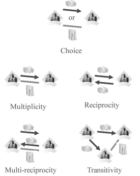
Figure 8: Basic and four other configurations. Possibility of these configurations is investigated in the analysis.

Choice configuration means the probability that exists either link between two nodes. Therefore, there are two $\lambda$s. By obtaining deviance for this base model, we can determine whether some other model with a single parameter has a larger difference in deviance to the base model than $\alpha$.

Multiplicity configuration, which is different from that of choice, means that both types of links between two nodes are represented, and one $\lambda$ is assigned. Therefore, this model reveals whether different types of links simultaneously emerge or not. The reciprocity configuration means that there are two-way transaction links between two nodes, and one $\lambda$ is assigned. The multi-reciprocity configuration also has a joint-patent application link.

The transitivity configuration represents the probability of links between three nodes. Other types of configurations between three nodes can be considered. However, this paper only presents the results for this configuration and the reasons will ee explained later. Suppose that the three nodes are called A, B and C; this configuration creates a situation where A and B, and A and C are connected by transaction links. In addition, B and C are connected by a joint-patent application link.

Table 2: $G^{2}_{PL}$ acquired with the $\mbox{p}^{*}$ model (First 20 industries)

Industry		Nodes	$\alpha$	Choice	Multi-	Recipro-	Multi-	Transi-
					plicity	city	reciprocity	tivity
(01)	Agriculture, forestry	5	-	-	-	-	-	-
	and fishery
(02)	Mining	72	8.9	2,282.8	2,230.6	2,212.6	2,269.3	2,281.1
					*	*	*
(03)	Foods	355	218.4	20,054.6	18,453.7	19,209.3	19,839.7	19,928.6
					*	*
(04)	Textile products	381	251.6	2,2823.9	21,923.0	22,137.5	22,744.5	22,731.4
					*	*
(05)	Pulp, paper and	242	101.4	10,872.0	10,133.7	10,547.3	10,799.2	10,784.2
	wooden products				*	*
(06)	Chemical products	1,104	2,116.4	112,351.0	107,759.2	108,230.3	11,562.7	110,612.2
					*	*
(07)	Petroleum and coal	119	24.4	5,077.1	4,847.1	4,981.8	5,057.3	4,987.4
	products				*	*		*
(08)	Ceramic, stone and	711	877.4	58,411.0	55,990.4	56,533.3	58,220.1	57,566.6
	clay products				*	*
(09)	Iron and steel	636	701.9	52,940.0	50,680.0	51,835.0	52,926.0	52,747.2
					*	*
(10)	Non-ferrous metals	521	470.9	43,581.2	42,079.3	42,356.9	43,390.6	43,101.6
					*	*		*
(11)	Metal products	875	1,329.1	72,567.8	67,557.4	70,268.63	71,690.4	70,830.1
					*	*		*
(12)	General machinery	1,554	4,194.5	166,446.0	158,330.2	162,082.9	165,777.5	163,636.7
					*	*
(13)	Electrical machinery	1,228	2,618.8	128,806.6	122,003.8	124,843.3	128,618.9	127,615.6
					*	*
(14)	Information and	499	431.9	39,865.0	37,677.1	38,530.7	39,763.2	39,586.67
	communication				*	*
	machinery
(15)	Electrical equipment	503	438.9	36,666.1	34,513.2	35,566.3	36,604.7	36,253.8
					*	*
(16)	Transportation	1,109	2,135.7	127,329.5	117,616.6	123,611.1	126,817.6	125,270.5
	equipment				*	*
(17)	Precision instruments	352	214.7	21,416.5	20,427.3	20,659.3	21,144.1	21,120.2
					*	*	*	*
(18)	Miscellaneous	1,096	2,085.9	93,997.5	89,052.7	90,924.2	93,542.2	92,539.2
	manufacturing				*	*
	products
(19)	Construction	1,021	1,810.0	129,410.3	123,297.5	127,415.4	129,206.0	127,446.1
					*	*		*
(20)	Electricity, gas	384	269.1	33,457.3	31,895.1	32,743.0	33,293.9	32,659.4
	and heat supply				*	*		*

Table 3: $G^{2}_{PL}$ acquired with the $\mbox{p}^{*}$ model (Last 14 industries)

Industry		Nodes	$\alpha$	Choice	Multi-	Recipro-	Multi-	Transi-
					plicity	city	reciprocity	tivity
(21)	Water supply	17	0.47	263.7	260.6	261.5	257.4	257.9
	and waste				*	*	*	*
	management services
(22)	Commerce	1,185	2,438.6	113,923.8	107,206.5	109,978.5	112,926.2	111,329.7
					*	*		*
(23)	Financial and insurance	257	114.3	13,985.6	13,766.6	13,619.7	13,852.2	13,890.5
					*	*	*
(24)	Real estate	136	31.9	5,686.5	5,564.9	5,572.9	5,678.1	5,677.9
					*	*
(25)	Transport	190	62.4	9,721.0	9,353.9	9,539.0	9,683.7	9,450.1
					*	*		*
(26)	Communication and	316	173.0	20,061.1	18,471.19	19,515.4	19,745.45	19,146.87
	broadcasting				*	*	*	*
(27)	Public administration	0	-	-	-	-	-	-
					*	*
(28)	Education and research	55	5.2	1,827.5	1,821.6	1,718.7	1,674.1	1,813.7
					*	*	*	*
(29)	Medical service, health	4	-	-	-	-	-	-
	and social security
	and nursing care
(30)	Other public services	0	-	-	-	-	-	-
(31)	Business services	639	708.6	45,513.8	43,030.3	44,346.8	45,182.0	44,674.8
					*	*		*
(32)	Personal services	5	-	-	-	-	-	-
(33)	Office supplies	0	-	-	-	-	-	-
(34)	Activities not elsewhere	0	-	-	-	-	-	-
	classified

Before analyzing the multi-layered network with the $\mbox{p}^{*}$ model, it should be divided into small parts and reduced by the number of nodes to decrease the calculation space. Consequently, the multi-layered network was divided into the industries presented in the previous section. By dividing the multi-layered network into the networks confined within industries, we can compare the common characteristics among the networks of industries.

Each node is classified by industry to divide a multi-layered network and transaction and joint-patent application links connected between different industries are omitted. Then, 34 separated multi-layered networks are created. The numbers of nodes in a network are reduced by separating them but some networks still have too many nodes.

A three-step process is conducted to futher reduce the number of nodes in networks. (1) Find a node with a maximum degree in joint-patent application links. If more than one node has a maximum degree, one of them is randomly chosen. (2) Select a connected graph by incrementing steps from the node in joint-patent application links. (3) Stop incrementing steps if there are no more connected nodes or the total number of nodes in the connected graph exceeds 1,000.

Tables 2 and 3 list the results of analyses obtained with the $\mbox{p}^{*}$ model. From the left of the tables, each column lists industries, nodes of connected graphs, and $\alpha$. Furthermore, the $G^{2}_{PL}$s for choice, multiplicity, reciprocity, multi-reciprocity and transitivity are given. If the differences between these $G^{2}_{PL}$s and that of choice are greater than $\alpha$, they are listed with asterisks. That means the model is significant.

As we can see from Tables 2 and 3, some industries do not have joint-patent application links, or have few links. Industries with fewer than 10 nodes were not analyzed.

Tables 2 and 3 indicate that multiplicity and reciprocity configurations are significant in all the analyzed industries. Multiplicity means transaction and joint-patent application links tend to emerge simultaneously, and reciprocity means two-way transaction links between two nodes tend to emerge simultaneously.

Multi-reciprocity and transitivity configurations, on the other hand, are significant in some of the analyzed industries. Multi-reciprocity is a mixture of multiplicity and reciprocity. The significance of multi-reciprocity is indicated in mining, precision instruments, water supply and waste management services, financial and insurance, communication and broadcasting, and education and research. Before conducting the analyses, the present author expected that significant configurations would appear in some specific industries that shared some characteristics. However, it is difficult to find any common characteristics in the listed industries. It is also difficult to find significance in transitivity in petroleum and coal products, non-ferrous metals, metal products, transportation equipment, construction, electricity, gas and head supply, water supply and waste management services, commerce, transport, communication and broadcasting, education and research, and business services. I could not find any common characteristics in the industries either. Hence, we can assume that other complicated configurations have the same tendency. This is why other complicated configurations were not analyzed.

With the analyses of the $\mbox{p}^{*}$ model explained in this section, I could not find common characteristics in industries in the analyses of configurations with three links or three nodes, and it is assumed that it was not worthwhile to investe other complicated configurations. However, the results for multiplicity are important. All analyzed industries indicated the significance of multiplicity, and this means that transactions and joint-patent application links are closely related. If there is a relationship between transaction and joint-patent application links between two nodes, the next question is which type of link precedes the other type. This wiil be discussed in the next section.

5 Bayesian networks

The relationship between transaction and joint-patent application links was revealed in Sections 3 and 4 at different levels, i.e., industries and firms. Consequently, whether either type of link tends to precede the other should be discussed. This question corresponds to the old question, do seeds precede needs, or do needs precede seeds?

The analysis of Bayesian networks is discussed in this section. Bayesian networks are completely different from the networks discussed in this paper thus far and these are methods to find causality from data.

A Bayesian network is a graphical model that encodes the joint probability distribution for a set of random variables. Some applications can be found in the overview by Lauritzen [14]. Bayesian networks were first proposed by Pearl [3]. Bayesian networks are used to fulfill three main objectives. They are to (1) infer unobserved variables, (2) to achieve parameter learning and (3) to accomplish structure learning.

Bayesian network can be used to infer unobserved variables because it is a model for variables and their relationships. Hence, by using some state of a subset of variables, Bayesian network updates the relationships and gives the joint probability distributions.

We often want to know the joint probability distributions among variables. This is parameter learning. It is necessary to specify the probability distribution for each node conditional on parents.

Structure learning is an advanced form of parameter learning. To acquire an expert’s way of thinking or to dissolve ambiguity in causality in variables, the network structure and parameters for joint probability distributions must be learned from the data. Therefore, structure learning exactly conforms to the objective of this section.

The method of structure learning is based on the idea proposed by Rebane and Pearl [15] and there are various kinds of improved methods. Deal is one methods propose by Bøttcher and Dethlefsen [16] and can be executed with R.

Figure 9 outlines the parameters for structure learning of Bayesian network. The parameters are defined for two firms. As seen in Figure 9, Industry A and B parameters are firms’ industries and if there is a joint-patent application link, the patent link parameter is set to 1, and if not, it is set to 0. If there is a transaction link from the firm of industry A to the firm of industry B, The transaction link parameter is set to 1, and if not, it is set to 0. Other parameters can be considered but Bayesian network built on four parameters is simple and easy to understand.

Figure 9: Parameters for structure learning of Bayesian network.

As the multi-layered network has 975,607 nodes, there are 975,607$\times$(975,606-1)$/$2 possible pairs. Since this is too large to calculate, pairs are chosen in four steps. (1) Choose one node randomly. (2) Acquire nodes that can traverse from the start node in a step with either link. (3) Consider all pairs from the chosen nodes. (4) Repeat (1) to (3) until enough pairs are acquired. This process is necessary because, as is intuitively understood, a randomly chosen pair is seldomly connected by links. By using the above process, 109,641 pairs are acquired.

Figure 10 outlines the results of structure learning conducted by deal. It seems that industries A and B precedes the transaction link and it precedes the patent link, but this is not true. From this structure, we can only learn that (1) the transaction and patent links are dependent. (2) The transaction link and industry A, and the transaction link and industry B are dependent. (3) If the value of the transaction link is given, the parameters, patent link, and industries A and B are independent. Since structure learning has limitations, the direction of dependence between transaction and joint-patent application links cannot be acquired. However, it is important for there to be many other possible structures and to choose the structure of the results from them. An example of the interpretation of results is where the possibility of a joint-patent application link between two firms only depends on a transaction link and the value of transaction links between any two firms is assessed in common. Therefore, we do not have to care about the industries of firms to know for the value of patent links.

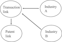
Figure 10: Bayesian network acquired by structure learning.

6 Conclusion

This paper investigated the relationship between transactions and cooperative R&D. Two different types of data were used. The first type was transaction data from Japanese firms. The network created from the data includes 961,363 firms and 7,808,760 links. The second type of data was joint-patent applications. The joint-patent application network included 54,197 nodes and 154,205 links. These two networks were merged into one network, called a multi-layered network. The network included 975,607 nodes and both types of links.

The first anaysis was based on input-output tables and three different tables were compared. The correleation coefficient between three pairs of tables were 0.31 (total amount of money and joint-patent applications), 0.45 (transactions and joint-patent applications) and 0.05 (transactions and the total amount of money). Transactions were found to be more strongly tied to joint-patent applications than the total amount of money. This means that the total amount of money can be used to track the scientific and technological connections to some degree, but transactions are more preferable to reach the objective. The total amount of money and transactions have few relationships and these are probably connected to the joint-patent applications in different mechanisms.

The second analysis was conducted based on the $\mbox{p}^{*}$ model. This revealed whether a network included significant configurations or not. The configurations of choice, multiplicity, reciprocity, multi-reciprocity and transitivity were evaluated. In this analysis, the multi-layered network was divided into industries. Multiplicity and reciprocity configurations were significant in all the analyzed industries. Multiplicity meant transactions and joint-patent application links tended to emerge simultaneously. The results for multiplicity meant that transactions and joint-patent application links were closely related. Reciprocity meant two-way transaction links between two nodes tended to emerge simultaneously. Multi-reciprocity and transitivity configurations were significant in some of the analyzed industries. It was difficult to find any common characteristics in the industries.

Bayesian networks were used in the third analysis. Bayesian networks are methods of finding causality from data and one usage is structure learning that can be executed by deal. The parameters were defined on two firms and they were Industries A and B, patent links and transaction links. By using the process of reducing pairs, 109,641 pairs were acquired. From the learned structure, we knew that (1) transaction links and patent links were dependent. (2) transaction links and Industry A and transaction links and Industry B were dependent. (3) If the value of a transaction link is given, the parameters of patent links and Industries A and B are independent.

7 Acknowledgements

This work was supported by KAKENHI (20730321).

References

- [1] W.W. Leontief. Input-Output Economics. Oxford University Press, New York, second edition, 1986.
- [2] S. Wasserman and G. Robins. An introduction to random graphs, dependence graphs, and p*. In P. J. Carrington, J. Scott, and S. Wasserman, editors, Models and Methods in Social Network Analysis, pages 148–161. Cambridge University Press, 2005.
- [3] J. Pearl. Causality. Cambridge University Press, New York, second edition, 2009.
- [4] H. Inoue, W. Souma, and S. Tamada. Analysis of cooperative research and development networks on Japanese patents. Informetrics, 4:89–96, 2010.
- [5] A. Clauset, C.R. Shalizi, and M.E.J. Newman. Power-law distributions in empirical data. SIAM Review, 51(4):661–703, 2009.
- [6] L. M. Koehly and P. Pattison. Random graph models for social networks: Multiple relations or multiple raters. In P.J. Carrington, J. Scott, and S. Wasserman, editors, Models and Methods in Social Network Analysis, chapter 9. Cambridge University Press, New York, 2005.
- [7] S. Wasserman. Conformity of two sociometric relations. Psychometrika, 52:3–18, 1987.
- [8] O. Frank and K. Nowicki. Exploratory statistical analysis of networks. In J. Gimbel, J.W. Kennedy, and L.V. Quintas, editors, Quo Vadis Graph Theory? A Source Book for Challenges and Directions. Amsterdam, 1993.
- [9] P. J. Carrington, J. Scott, and S. Wasserman, editors. Models and Methods in Social Network Analysis. Cambridge university press, 2005.
- [10] J. E. Besag. Statistical analysis of non-lattice data. The Statistician, 24:179–195, 1975.
- [11] J. E. Besag. Some methods of statistical analysis for spatial data. Bulletin of the International Statistical Association, 47:77–92, 1977.
- [12] D. Strauss and M. Ikeda. Pseudolikelihood estimation for social networks. Journal of the American Statistical Association, 85:204–212, 1990.
- [13] P. Pattison and S. Wasserman. Logit models and logistic regressions for social networks: II. multivariate relations. British Journal of Mathematical and Statistical Psychology, 52:169–193, 1999.
- [14] S.L. Lauritzen. Some modern applications of graphical models. In P.J. Green, N.L. Hjort, and S. Richardson, editors, Highly Structured Stochastic Systems. Oxford University Press, 2003.
- [15] G. Rebane and J. Pearl. The recovery of causal poly-trees from statistical data. In Proceedings of 3rd workshop on uncertainty in AI, pages 222–228, 1987.
- [16] S.G. Bøttcher and C. Dethlefsen. deal: A package for learning bayesian networks. Journal of statistical software, 8(Issue 20), 2003.