1 Introduction
In one-dimensional quantum systems, a completely different behavior
for the integer spin
chains from the half-integer spin chains was predicted by Haldane
[1 , 2 ] .
The antiferromagnetic isotropic
spin-1 model introduced by Affleck, Kennedy, Lieb and Tasaki
(AKLT model) [3 ] ,
whose ground state can be exactly calculated, has been a useful toy model
to validate Haldane’s prediction of the massive behavior
for integer spin chains.
Moreover, it lead to a deeper understanding for integer spin chains such as the
discovery of the special type of long-range order [4 , 5 ] .
The AKLT model has been generalized to
higher-spin models,
anisotropic models, etc
[6 , 7 , 8 , 9 , 10 , 11 , 12 , 13 , 14 , 15 , 16 , 17 ] .
The Hamiltonians are essentially linear combinations
of projection operators with nonnegative coefficients,
and their ground states are called valence-bond-solid (VBS) state.
Recently, the VBS state was investigated
in perspective of
its relation to quantum information and experimental implementation
by means of optical lattices,
see Refs. [18 , 19 ] for example.
There are largely three types of representations for the ground state which
are equivalent to each other:
the Schwinger boson representation, the spin coherent
representation and the matrix product representation.
For isotropic higher-spin models,
the spin-spin correlation functions [20 ]
and the entanglement entropy [21 , 22 ]
have been calculated by utilizing the spin coherent representation
and the properties of Legendre polynomials.
For the q 𝑞 q [7 , 8 , 9 ]
from the matrix product representation.
In this paper, we consider the ground state of
a q 𝑞 q [24 ] (q 𝑞 q q 𝑞 q
This paper is organized as follows.
In the next section, we briefly review
the quantum group U q ( s u ( 2 ) ) subscript 𝑈 𝑞 𝑠 𝑢 2 U_{q}(su(2)) 3 q 𝑞 q L 𝐿 L q 𝑞 q L 𝐿 L G 𝐺 G 4 G 𝐺 G 5 6
2 The quantum group U q ( s u ( 2 ) ) subscript 𝑈 𝑞 𝑠 𝑢 2 U_{q}(su(2))
We introduce several notations,
fixing a real number q 𝑞 q q 𝑞 q q 𝑞 q q 𝑞 q N ∈ ℤ ≥ 0 𝑁 subscript ℤ absent 0 N\in{\mathbb{Z}}_{\geq 0}
[ N ] = q N − q − N q − q − 1 , [ N ] ! = { ∏ I = 1 N [ I ] N ∈ ℕ , 1 N = 0 , [ N K ] = { [ N ] ! [ K ] ! [ N − K ] ! K = 0 , … , N , 0 otherwise , \displaystyle\begin{split}[N]=\frac{q^{N}-q^{-N}}{q-q^{-1}},\quad[N]!=\begin{cases}\displaystyle\prod_{I=1}^{N}[I]&N\in{\mathbb{N}},\\
1&N=0,\end{cases}\\
\left[\begin{array}[]{c}N\\
K\end{array}\right]=\begin{cases}\displaystyle\frac{[N]!}{[K]![N-K]!}&K=0,\dots,N,\\
0&\rm otherwise,\end{cases}\end{split} (2.1)
respectively.
The quantum group U q ( s u ( 2 ) ) subscript 𝑈 𝑞 𝑠 𝑢 2 U_{q}(su(2)) [25 , 26 ]
is defined by generators X + , X − superscript 𝑋 superscript 𝑋
X^{+},X^{-} H 𝐻 H
[ X + , X − ] = q H − q − H q − q − 1 , [ H , X ± ] = ± 2 X ± . formulae-sequence superscript 𝑋 superscript 𝑋 superscript 𝑞 𝐻 superscript 𝑞 𝐻 𝑞 superscript 𝑞 1 𝐻 superscript 𝑋 plus-or-minus plus-or-minus 2 superscript 𝑋 plus-or-minus \displaystyle\left[X^{+},X^{-}\right]=\frac{q^{H}-q^{-H}}{q-q^{-1}},\quad\left[H,X^{\pm}\right]=\pm 2X^{\pm}. (2.2)
The comultiplication is given by
Δ ( X ± ) = X ± ⊗ q H / 2 + q − H / 2 ⊗ X ± , Δ ( H ) = H ⊗ Id + Id ⊗ H . formulae-sequence Δ superscript 𝑋 plus-or-minus tensor-product superscript 𝑋 plus-or-minus superscript 𝑞 𝐻 2 tensor-product superscript 𝑞 𝐻 2 superscript 𝑋 plus-or-minus Δ 𝐻 tensor-product 𝐻 Id tensor-product Id 𝐻 \displaystyle\Delta\left(X^{\pm}\right)=X^{\pm}\otimes q^{H/2}+q^{-H/2}\otimes X^{\pm},\quad\Delta(H)=H\otimes\mathrm{Id}+\mathrm{Id}\otimes H. (2.3)
U q ( s u ( 2 ) ) subscript 𝑈 𝑞 𝑠 𝑢 2 U_{q}(su(2))
X + = a † b , X − = b † a , H = N a − N b , formulae-sequence superscript 𝑋 superscript 𝑎 † 𝑏 formulae-sequence superscript 𝑋 superscript 𝑏 † 𝑎 𝐻 subscript 𝑁 𝑎 subscript 𝑁 𝑏 \displaystyle X^{+}=a^{\dagger}b,\quad X^{-}=b^{\dagger}a,\quad H=N_{a}-N_{b}, (2.4)
with q 𝑞 q a 𝑎 a b 𝑏 b
a a † − q a † a = q − N a , b b † − q b † b = q − N b , formulae-sequence 𝑎 superscript 𝑎 † 𝑞 superscript 𝑎 † 𝑎 superscript 𝑞 subscript 𝑁 𝑎 𝑏 superscript 𝑏 † 𝑞 superscript 𝑏 † 𝑏 superscript 𝑞 subscript 𝑁 𝑏 \displaystyle aa^{\dagger}-qa^{\dagger}a=q^{-N_{a}},\quad bb^{\dagger}-qb^{\dagger}b=q^{-N_{b}}, (2.5)
[ N a , a ] = − a , [ N a , a † ] = a † , [ N b , b ] = − b , [ N b , b † ] = b † . formulae-sequence subscript 𝑁 𝑎 𝑎 𝑎 formulae-sequence subscript 𝑁 𝑎 superscript 𝑎 † superscript 𝑎 † formulae-sequence subscript 𝑁 𝑏 𝑏 𝑏 subscript 𝑁 𝑏 superscript 𝑏 † superscript 𝑏 † \displaystyle[N_{a},a]=-a,\quad[N_{a},a^{\dagger}]=a^{\dagger},\quad[N_{b},b]=-b,\quad[N_{b},b^{\dagger}]=b^{\dagger}. (2.6)
We denote the space where ( 2 j + 1 ) 2 𝑗 1 (2j+1) U q ( s u ( 2 ) ) subscript 𝑈 𝑞 𝑠 𝑢 2 U_{q}(su(2)) V j subscript 𝑉 𝑗 V_{j} V j subscript 𝑉 𝑗 V_{j}
| j ; m ⟩ = ( a † ) j + m ( b † ) j − m [ j + m ] ! [ j − m ] ! | vac ⟩ , ( m = − j , … , j ) . ket 𝑗 𝑚
superscript superscript 𝑎 † 𝑗 𝑚 superscript superscript 𝑏 † 𝑗 𝑚 delimited-[] 𝑗 𝑚 delimited-[] 𝑗 𝑚 ket vac 𝑚 𝑗 … 𝑗
\displaystyle|j;m{\rangle}=\frac{(a^{\dagger})^{j+m}(b^{\dagger})^{j-m}}{\sqrt{[j+m]![j-m]!}}|\mathrm{vac}{\rangle},\ \ (m=-j,\dots,j). (2.7)
The Weyl representation which we describe below,
is an equivalent representation to
the Schwinger boson representation,
and is efficient for practical calculation.
Let us denote the q 𝑞 q a 𝑎 a b 𝑏 b α 𝛼 \alpha a α subscript 𝑎 𝛼 a_{\alpha} b α subscript 𝑏 𝛼 b_{\alpha} a α † superscript subscript 𝑎 𝛼 † a_{\alpha}^{\dagger} b α † superscript subscript 𝑏 𝛼 † b_{\alpha}^{\dagger} a α subscript 𝑎 𝛼 a_{\alpha} b α subscript 𝑏 𝛼 b_{\alpha} ℂ [ x α , y α ] ℂ subscript 𝑥 𝛼 subscript 𝑦 𝛼 \mathbb{C}[x_{\alpha},y_{\alpha}]
a α † = x α , b α † = y α , a α = 1 x α D q x α − D q − 1 x α q − q − 1 , b α = 1 y α D q y α − D q − 1 y α q − q − 1 , formulae-sequence superscript subscript 𝑎 𝛼 † subscript 𝑥 𝛼 formulae-sequence superscript subscript 𝑏 𝛼 † subscript 𝑦 𝛼 formulae-sequence subscript 𝑎 𝛼 1 subscript 𝑥 𝛼 superscript subscript 𝐷 𝑞 subscript 𝑥 𝛼 superscript subscript 𝐷 superscript 𝑞 1 subscript 𝑥 𝛼 𝑞 superscript 𝑞 1 subscript 𝑏 𝛼 1 subscript 𝑦 𝛼 superscript subscript 𝐷 𝑞 subscript 𝑦 𝛼 superscript subscript 𝐷 superscript 𝑞 1 subscript 𝑦 𝛼 𝑞 superscript 𝑞 1 \displaystyle a_{\alpha}^{\dagger}=x_{\alpha},\quad b_{\alpha}^{\dagger}=y_{\alpha},\quad a_{\alpha}=\frac{1}{x_{\alpha}}\frac{D_{q}^{x_{\alpha}}-D_{q^{-1}}^{x_{\alpha}}}{q-q^{-1}},\ \ b_{\alpha}=\frac{1}{y_{\alpha}}\frac{D_{q}^{y_{\alpha}}-D_{q^{-1}}^{y_{\alpha}}}{q-q^{-1}}, (2.8)
where
D p x α f ( x α , y α ) = f ( p x α , y α ) , D p y α f ( x α , y α ) = f ( x α , p y α ) . formulae-sequence superscript subscript 𝐷 𝑝 subscript 𝑥 𝛼 𝑓 subscript 𝑥 𝛼 subscript 𝑦 𝛼 𝑓 𝑝 subscript 𝑥 𝛼 subscript 𝑦 𝛼 superscript subscript 𝐷 𝑝 subscript 𝑦 𝛼 𝑓 subscript 𝑥 𝛼 subscript 𝑦 𝛼 𝑓 subscript 𝑥 𝛼 𝑝 subscript 𝑦 𝛼 \displaystyle D_{p}^{x_{\alpha}}f(x_{\alpha},y_{\alpha})=f(px_{\alpha},y_{\alpha}),\ \ D_{p}^{y_{\alpha}}f(x_{\alpha},y_{\alpha})=f(x_{\alpha},py_{\alpha}). (2.9)
The generators of U q ( s u ( 2 ) ) subscript 𝑈 𝑞 𝑠 𝑢 2 U_{q}(su(2))
X α + = x α y α D q y α − D q − 1 y α q − q − 1 , X α − = y α x α D q x α − D q − 1 x α q − q − 1 , q H α = D q x α D q − 1 y α . formulae-sequence subscript superscript 𝑋 𝛼 subscript 𝑥 𝛼 subscript 𝑦 𝛼 superscript subscript 𝐷 𝑞 subscript 𝑦 𝛼 subscript superscript 𝐷 subscript 𝑦 𝛼 superscript 𝑞 1 𝑞 superscript 𝑞 1 formulae-sequence subscript superscript 𝑋 𝛼 subscript 𝑦 𝛼 subscript 𝑥 𝛼 superscript subscript 𝐷 𝑞 subscript 𝑥 𝛼 subscript superscript 𝐷 subscript 𝑥 𝛼 superscript 𝑞 1 𝑞 superscript 𝑞 1 superscript 𝑞 subscript 𝐻 𝛼 subscript superscript 𝐷 subscript 𝑥 𝛼 𝑞 subscript superscript 𝐷 subscript 𝑦 𝛼 superscript 𝑞 1 \displaystyle X^{+}_{\alpha}=\frac{x_{\alpha}}{y_{\alpha}}\frac{D_{q}^{y_{\alpha}}-D^{y_{\alpha}}_{q^{-1}}}{q-q^{-1}},\ X^{-}_{\alpha}=\frac{y_{\alpha}}{x_{\alpha}}\frac{D_{q}^{x_{\alpha}}-D^{x_{\alpha}}_{q^{-1}}}{q-q^{-1}},\ q^{H_{\alpha}}=D^{x_{\alpha}}_{q}D^{y_{\alpha}}_{q^{-1}}. (2.10)
The tensor product of two irreducible representations has the
Clebsch-Gordan decomposition
V S ⊗ V S tensor-product subscript 𝑉 𝑆 subscript 𝑉 𝑆 \displaystyle V_{S}\otimes V_{S} = ⨁ J = 0 2 S V J , absent superscript subscript direct-sum 𝐽 0 2 𝑆 subscript 𝑉 𝐽 \displaystyle=\bigoplus_{J=0}^{2S}V_{J}, (2.11)
| S ; m 1 ⟩ ⊗ | S ; m 2 ⟩ tensor-product ket 𝑆 subscript 𝑚 1
ket 𝑆 subscript 𝑚 2
\displaystyle|S;m_{1}\rangle\otimes|S;m_{2}\rangle = ∑ J = 0 2 S [ S S J m 1 m 2 m 1 + m 2 ] | J ; m 1 + m 2 ⟩ , absent superscript subscript 𝐽 0 2 𝑆 delimited-[] 𝑆 𝑆 𝐽 subscript 𝑚 1 subscript 𝑚 2 subscript 𝑚 1 subscript 𝑚 2 ket 𝐽 subscript 𝑚 1 subscript 𝑚 2
\displaystyle=\sum_{J=0}^{2S}\left[\begin{array}[]{ccc}S&S&J\\
m_{1}&m_{2}&m_{1}+m_{2}\end{array}\right]|J;m_{1}+m_{2}\rangle, (2.14)
where
[ S 1 S 2 J m 1 m 2 m ] = δ m 1 + m 2 , m ( − 1 ) S 1 − m 1 q m 1 ( m 1 + m 2 + 1 ) + { S 2 ( S 2 + 1 ) − S 1 ( S 1 + 1 ) − J ( J + 1 ) } / 2 delimited-[] subscript 𝑆 1 subscript 𝑆 2 𝐽 subscript 𝑚 1 subscript 𝑚 2 𝑚 subscript 𝛿 subscript 𝑚 1 subscript 𝑚 2 𝑚
superscript 1 subscript 𝑆 1 subscript 𝑚 1 superscript 𝑞 subscript 𝑚 1 subscript 𝑚 1 subscript 𝑚 2 1 subscript 𝑆 2 subscript 𝑆 2 1 subscript 𝑆 1 subscript 𝑆 1 1 𝐽 𝐽 1 2 \displaystyle\left[\begin{array}[]{ccc}S_{1}&S_{2}&J\\
m_{1}&m_{2}&m\end{array}\right]=\delta_{m_{1}+m_{2},m}(-1)^{S_{1}-m_{1}}q^{m_{1}(m_{1}+m_{2}+1)+\{S_{2}(S_{2}+1)-S_{1}(S_{1}+1)-J(J+1)\}/2} (2.17)
× [ J + m ] ! [ J − m ] ! [ S 1 − m 1 ] ! [ S 2 − m 2 ] ! [ S 1 + S 2 − J ] ! [ 2 J + 1 ] [ S 1 + m 1 ] ! [ S 2 + m 2 ] ! [ S 1 − S 2 + J ] ! [ S 2 − S 1 + J ] ! [ S 1 + S 2 + J + 1 ] ! absent delimited-[] 𝐽 𝑚 delimited-[] 𝐽 𝑚 delimited-[] subscript 𝑆 1 subscript 𝑚 1 delimited-[] subscript 𝑆 2 subscript 𝑚 2 delimited-[] subscript 𝑆 1 subscript 𝑆 2 𝐽 delimited-[] 2 𝐽 1 delimited-[] subscript 𝑆 1 subscript 𝑚 1 delimited-[] subscript 𝑆 2 subscript 𝑚 2 delimited-[] subscript 𝑆 1 subscript 𝑆 2 𝐽 delimited-[] subscript 𝑆 2 subscript 𝑆 1 𝐽 delimited-[] subscript 𝑆 1 subscript 𝑆 2 𝐽 1 \displaystyle\times\sqrt{\frac{[J+m]![J-m]![S_{1}-m_{1}]![S_{2}-m_{2}]![S_{1}+S_{2}-J]![2J+1]}{[S_{1}+m_{1}]![S_{2}+m_{2}]![S_{1}-S_{2}+J]![S_{2}-S_{1}+J]![S_{1}+S_{2}+J+1]!}} (2.18)
× ∑ z = Max ( 0 , − S 1 − m 1 , J − S 2 − m 1 ) Min ( J − m , S 1 − m 1 , S 2 + J − m 1 ) ( − q m + J + 1 ) z [ S 1 + m 1 + z ] ! [ S 2 + J − m 1 − z ] ! [ z ] ! [ J − m − z ] ! [ S 1 − m 1 − z ] ! [ S 2 − J + m 1 + z ] ! , \displaystyle\times\sum_{z=\mathrm{Max}(0,-S_{1}-m_{1},J-S_{2}-m_{1})}^{\mathrm{Min}(J-m,S_{1}-m_{1},S_{2}+J-m_{1})}\frac{(-q^{m+J+1})^{z}[S_{1}+m_{1}+z]![S_{2}+J-m_{1}-z]!}{[z]![J-m-z]![S_{1}-m_{1}-z]![S_{2}-J+m_{1}+z]!},
is the q 𝑞 q [23 ] .
(The factor q m 1 m 2 / 2 superscript 𝑞 subscript 𝑚 1 subscript 𝑚 2 2 q^{m_{1}m_{2}/2} [23 ] .)
This coefficient
is compatible with the inverse
of the decomposition (2.14
| J ; m ⟩ = ∑ m 1 + m 2 = m [ S S J m 1 m 2 m 1 + m 2 ] | S ; m 1 ⟩ ⊗ | S ; m 2 ⟩ . ket 𝐽 𝑚
subscript subscript 𝑚 1 subscript 𝑚 2 𝑚 tensor-product delimited-[] 𝑆 𝑆 𝐽 subscript 𝑚 1 subscript 𝑚 2 subscript 𝑚 1 subscript 𝑚 2 ket 𝑆 subscript 𝑚 1
ket 𝑆 subscript 𝑚 2
\displaystyle|J;m\rangle=\sum_{m_{1}+m_{2}=m}\left[\begin{array}[]{ccc}S&S&J\\
m_{1}&m_{2}&m_{1}+m_{2}\end{array}\right]|S;m_{1}\rangle\otimes|S;m_{2}\rangle. (2.21)
For later purpose, we will also
investigate the Clebsch-Gordan decomposition
of U q ( s u ( 2 ) ) subscript 𝑈 𝑞 𝑠 𝑢 2 U_{q}(su(2))
Δ X α β ± = Δ subscript superscript 𝑋 plus-or-minus 𝛼 𝛽 absent \displaystyle\Delta X^{\pm}_{\alpha\beta}= X α ± ⊗ q H β / 2 + q − H α / 2 ⊗ X β ± , tensor-product subscript superscript 𝑋 plus-or-minus 𝛼 superscript 𝑞 subscript 𝐻 𝛽 2 tensor-product superscript 𝑞 subscript 𝐻 𝛼 2 subscript superscript 𝑋 plus-or-minus 𝛽 \displaystyle X^{\pm}_{\alpha}\otimes q^{H_{\beta}/2}+q^{-H_{\alpha}/2}\otimes X^{\pm}_{\beta}, (2.22)
one can show that the highest weight vector
v J ∈ V J ( Δ X + v J = 0 ) subscript 𝑣 𝐽 subscript 𝑉 𝐽 Δ superscript 𝑋 subscript 𝑣 𝐽 0 v_{J}\in V_{J}\ (\Delta X^{+}v_{J}=0) α 𝛼 \alpha β 𝛽 \beta
v J = ( x α x β ) J ∏ ν = 1 2 S − J ( x α y β − q 2 ( ν − S − 1 ) x β y α ) . subscript 𝑣 𝐽 superscript subscript 𝑥 𝛼 subscript 𝑥 𝛽 𝐽 superscript subscript product 𝜈 1 2 𝑆 𝐽 subscript 𝑥 𝛼 subscript 𝑦 𝛽 superscript 𝑞 2 𝜈 𝑆 1 subscript 𝑥 𝛽 subscript 𝑦 𝛼 \displaystyle v_{J}=(x_{\alpha}x_{\beta})^{J}\prod_{\nu=1}^{2S-J}(x_{\alpha}y_{\beta}-q^{2(\nu-S-1)}x_{\beta}y_{\alpha}). (2.23)
Moreover, we can show the following:
Proposition 2.1 .
( Δ X α β − ) n v J = ( x α x β ) J − n q n S [ n ] ! ∑ μ = 0 n q − 2 μ S [ J μ ] [ J n − μ ] ( x α y β ) μ ( x β y α ) n − μ × ∏ ν = 1 2 S − J ( x α y β − q 2 ( ν − S − 1 ) x β y α ) . superscript Δ subscript superscript 𝑋 𝛼 𝛽 𝑛 subscript 𝑣 𝐽 superscript subscript 𝑥 𝛼 subscript 𝑥 𝛽 𝐽 𝑛 superscript 𝑞 𝑛 𝑆 delimited-[] 𝑛 superscript subscript 𝜇 0 𝑛 superscript 𝑞 2 𝜇 𝑆 delimited-[] 𝐽 𝜇 delimited-[] 𝐽 𝑛 𝜇 superscript subscript 𝑥 𝛼 subscript 𝑦 𝛽 𝜇 superscript subscript 𝑥 𝛽 subscript 𝑦 𝛼 𝑛 𝜇 superscript subscript product 𝜈 1 2 𝑆 𝐽 subscript 𝑥 𝛼 subscript 𝑦 𝛽 superscript 𝑞 2 𝜈 𝑆 1 subscript 𝑥 𝛽 subscript 𝑦 𝛼 \displaystyle\begin{split}\left(\Delta X^{-}_{\alpha\beta}\right)^{n}v_{J}=&(x_{\alpha}x_{\beta})^{J-n}q^{nS}[n]!\sum_{\mu=0}^{n}q^{-2\mu S}\left[\begin{array}[]{c}J\\
\mu\end{array}\right]\left[\begin{array}[]{c}J\\
n-\mu\end{array}\right]\left(x_{\alpha}y_{\beta}\right)^{\mu}\left(x_{\beta}y_{\alpha}\right)^{n-\mu}\\
&\times\prod_{\nu=1}^{2S-J}\left(x_{\alpha}y_{\beta}-q^{2(\nu-S-1)}x_{\beta}y_{\alpha}\right).\end{split} (2.24)
A proof of this proposition
is given in Appendix A
3 q 𝑞 q
The model we treat in this paper
is an anisotropic integer spin-S 𝑆 S L 𝐿 L
ℋ = ∑ k ∈ ℤ L ∑ J = S + 1 2 S C J ( k , k + 1 ) ( π J ) k , k + 1 , ℋ subscript 𝑘 subscript ℤ 𝐿 superscript subscript 𝐽 𝑆 1 2 𝑆 subscript 𝐶 𝐽 𝑘 𝑘 1 subscript subscript 𝜋 𝐽 𝑘 𝑘 1
\displaystyle{\mathcal{H}}=\sum_{k\in{\mathbb{Z}}_{L}}\sum_{J=S+1}^{2S}C_{J}(k,k+1)\left(\pi_{J}\right)_{k,k+1}, (3.1)
where C J ( k , k + 1 ) > 0 subscript 𝐶 𝐽 𝑘 𝑘 1 0 C_{J}(k,k+1)>0 ( π J ) k , k + 1 subscript subscript 𝜋 𝐽 𝑘 𝑘 1
\left(\pi_{J}\right)_{k,k+1} k 𝑘 k ( k + 1 ) 𝑘 1 (k+1) U q ( s u ( 2 ) ) subscript 𝑈 𝑞 𝑠 𝑢 2 U_{q}(su(2)) V S ⊗ V S tensor-product subscript 𝑉 𝑆 subscript 𝑉 𝑆 V_{S}\otimes V_{S} V J subscript 𝑉 𝐽 V_{J}
π J = ∑ m 1 , m 2 , m 1 ′ , m 2 ′ = − S S [ S S J m 1 m 2 m 1 + m 2 ] [ S S J m 1 ′ m 2 ′ m 1 ′ + m 2 ′ ] × δ m 1 + m 2 , m 1 ′ + m 2 ′ | S ; m 1 ′ ⟩ ⟨ S ; m 1 | ⊗ | S ; m 2 ′ ⟩ ⟨ S ; m 2 | . \displaystyle\begin{split}\pi_{J}=&\sum_{m_{1},m_{2},m_{1}^{\prime},m_{2}^{\prime}=-S}^{S}\left[\begin{array}[]{ccc}S&S&J\\
m_{1}&m_{2}&m_{1}+m_{2}\end{array}\right]\left[\begin{array}[]{ccc}S&S&J\\
m_{1}^{\prime}&m_{2}^{\prime}&m_{1}^{\prime}+m_{2}^{\prime}\end{array}\right]\\
&\quad\quad\times\delta_{m_{1}+m_{2},m_{1}^{\prime}+m_{2}^{\prime}}|S;m_{1}^{\prime}\rangle\langle S;m_{1}|\otimes|S;m_{2}^{\prime}\rangle\langle S;m_{2}|.\end{split} (3.2)
The nonnegativity
⟨ ψ | ( π J ) k , k + 1 | ψ ⟩ ≥ 0 ( for any vector | ψ ⟩ ) quantum-operator-product 𝜓 subscript subscript 𝜋 𝐽 𝑘 𝑘 1
𝜓 0 for any vector ket 𝜓
\displaystyle\langle\psi|\left(\pi_{J}\right)_{k,k+1}|\psi\rangle\geq 0\quad\left(\text{for any vector }|\psi\rangle\right) (3.3)
implies that all the eigenvalues of ℋ ℋ \mathcal{H} ⟨ ψ | bra 𝜓 \langle\psi| | ψ ⟩ ket 𝜓 |\psi\rangle | Ψ ⟩ ket Ψ |\Psi\rangle
ℋ | Ψ ⟩ = 0 . ℋ ket Ψ 0 \displaystyle\mathcal{H}|\Psi\rangle=0. (3.4)
Since we set C J ( k , k + 1 ) > 0 subscript 𝐶 𝐽 𝑘 𝑘 1 0 C_{J}(k,k+1)>0 3.4
( π J ) k , k + 1 | Ψ ⟩ = 0 ( ∀ k ∈ ℤ L , ∀ J ∈ { S + 1 , … , 2 S } ) , subscript subscript 𝜋 𝐽 𝑘 𝑘 1
ket Ψ 0 formulae-sequence for-all 𝑘 subscript ℤ 𝐿 for-all 𝐽 𝑆 1 … 2 𝑆
\displaystyle\left(\pi_{J}\right)_{k,k+1}|\Psi\rangle=0\quad\left(\forall k\in{\mathbb{Z}}_{L},\ \forall J\in\{S+1,\dots,2S\}\right), (3.5)
noting the nonnegativity (3.3 2.1 ⨁ 0 ≤ J ≤ S V J ⊂ V S ⊗ V S subscript direct-sum 0 𝐽 𝑆 subscript 𝑉 𝐽 tensor-product subscript 𝑉 𝑆 subscript 𝑉 𝑆 \bigoplus_{0\leq J\leq S}V_{J}\subset V_{S}\otimes V_{S} k 𝑘 k ( k + 1 ) 𝑘 1 (k+1)
∑ 0 ≤ A , B ≤ S C A B x k A y k S − A x k + 1 B y k + 1 S − B ∏ m = 1 S ( q m x k y k + 1 − q − m y k x k + 1 ) , subscript formulae-sequence 0 𝐴 𝐵 𝑆 subscript 𝐶 𝐴 𝐵 superscript subscript 𝑥 𝑘 𝐴 superscript subscript 𝑦 𝑘 𝑆 𝐴 superscript subscript 𝑥 𝑘 1 𝐵 superscript subscript 𝑦 𝑘 1 𝑆 𝐵 superscript subscript product 𝑚 1 𝑆 superscript 𝑞 𝑚 subscript 𝑥 𝑘 subscript 𝑦 𝑘 1 superscript 𝑞 𝑚 subscript 𝑦 𝑘 subscript 𝑥 𝑘 1 \displaystyle\sum_{0\leq A,B\leq S}C_{AB}x_{k}^{A}y_{k}^{S-A}x_{k+1}^{B}y_{k+1}^{S-B}\prod_{m=1}^{S}(q^{m}x_{k}y_{k+1}-q^{-m}y_{k}x_{k+1}), (3.6)
where C A B subscript 𝐶 𝐴 𝐵 C_{AB} x k , y k , x k + 1 subscript 𝑥 𝑘 subscript 𝑦 𝑘 subscript 𝑥 𝑘 1
x_{k},y_{k},x_{k+1} y k + 1 subscript 𝑦 𝑘 1 y_{k+1} 3.5 | Ψ ⟩ ket Ψ |\Psi\rangle
| Ψ ⟩ = P ( { x k } k ∈ ℤ L , { y k } k ∈ ℤ L ) ∏ k ∈ ℤ L ∏ m = 1 S ( q m x k y k + 1 − q − m y k x k + 1 ) ket Ψ 𝑃 subscript subscript 𝑥 𝑘 𝑘 subscript ℤ 𝐿 subscript subscript 𝑦 𝑘 𝑘 subscript ℤ 𝐿 subscript product 𝑘 subscript ℤ 𝐿 superscript subscript product 𝑚 1 𝑆 superscript 𝑞 𝑚 subscript 𝑥 𝑘 subscript 𝑦 𝑘 1 superscript 𝑞 𝑚 subscript 𝑦 𝑘 subscript 𝑥 𝑘 1 \displaystyle|\Psi{\rangle}=P\left(\{x_{k}\}_{k\in{\mathbb{Z}}_{L}},\{y_{k}\}_{k\in{\mathbb{Z}}_{L}}\right)\prod_{k\in{\mathbb{Z}}_{L}}\prod_{m=1}^{S}(q^{m}x_{k}y_{k+1}-q^{-m}y_{k}x_{k+1}) (3.7)
with some polynomials P 𝑃 P 3.6 ∀ k ∈ ℤ L for-all 𝑘 subscript ℤ 𝐿 \forall k\in{\mathbb{Z}}_{L} P 𝑃 P
| Ψ ⟩ = ∏ k ∈ ℤ L ∏ m = 1 S ( q m x k y k + 1 − q − m y k x k + 1 ) . ket Ψ subscript product 𝑘 subscript ℤ 𝐿 superscript subscript product 𝑚 1 𝑆 superscript 𝑞 𝑚 subscript 𝑥 𝑘 subscript 𝑦 𝑘 1 superscript 𝑞 𝑚 subscript 𝑦 𝑘 subscript 𝑥 𝑘 1 \displaystyle|\Psi{\rangle}=\prod_{k\in{\mathbb{Z}}_{L}}\prod_{m=1}^{S}(q^{m}x_{k}y_{k+1}-q^{-m}y_{k}x_{k+1}). (3.8)
In the Schwinger boson representation, we have
| Ψ ⟩ = ∏ k ∈ ℤ L ∏ m = 1 S ( q m a k † b k + 1 † − q − m b k † a k + 1 † ) | vac ⟩ , ket Ψ subscript product 𝑘 subscript ℤ 𝐿 superscript subscript product 𝑚 1 𝑆 superscript 𝑞 𝑚 superscript subscript 𝑎 𝑘 † superscript subscript 𝑏 𝑘 1 † superscript 𝑞 𝑚 superscript subscript 𝑏 𝑘 † superscript subscript 𝑎 𝑘 1 † ket vac \displaystyle|\Psi{\rangle}=\prod_{k\in{\mathbb{Z}}_{L}}\prod_{m=1}^{S}(q^{m}a_{k}^{\dagger}b_{k+1}^{\dagger}-q^{-m}b_{k}^{\dagger}a_{k+1}^{\dagger})|\mathrm{vac}{\rangle}, (3.9)
which is a generalization of the q = 1 𝑞 1 q=1 [6 ] .
Note that each site have the correct spin value:
N k | Ψ ⟩ = S | Ψ ⟩ subscript 𝑁 𝑘 ket Ψ 𝑆 ket Ψ N_{k}|\Psi\rangle=S|\Psi\rangle k ∈ ℤ L 𝑘 subscript ℤ 𝐿 k\in{\mathbb{Z}}_{L} N k := ( N a k + N b k ) / 2 assign subscript 𝑁 𝑘 subscript 𝑁 subscript 𝑎 𝑘 subscript 𝑁 subscript 𝑏 𝑘 2 N_{k}:=(N_{a_{k}}+N_{b_{k}})/2 q 𝑞 q q 𝑞 q 1
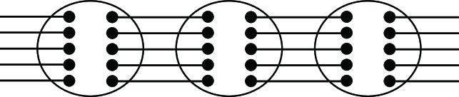
Figure 1: Conceptual figure of the q 𝑞 q q 𝑞 q ○ ○ \bigcirc q 𝑞 q ∙ ∙ \bullet
The Schwinger boson representation
of the ground state (3.9 [24 ] , which
generalizes the q = 1 𝑞 1 q=1 [27 ] or S = 1 𝑆 1 S=1 [7 ] case.
Noting (2.7
| Ψ ⟩ ket Ψ \displaystyle|\Psi\rangle = Tr [ g 1 ⋆ g 2 ⋆ ⋯ ⋆ g L − 1 ⋆ g L ] , absent Tr delimited-[] ⋆ subscript 𝑔 1 subscript 𝑔 2 ⋯ subscript 𝑔 𝐿 1 subscript 𝑔 𝐿 \displaystyle=\mathrm{Tr}[g_{1}\star g_{2}\star\cdots\star g_{L-1}\star g_{L}], (3.10)
where
g k subscript 𝑔 𝑘 g_{k} ( S + 1 ) × ( S + 1 ) 𝑆 1 𝑆 1 (S+1)\times(S+1) k 𝑘 k
g k ( i , i ′ ) = ( − 1 ) S − i q ( i + i ′ − S ) ( S + 1 ) / 2 [ S i ] [ S i ′ ] [ S − i + i ′ ] ! [ S + i − i ′ ] ! | S ; i ′ − i ⟩ k = : h i i ′ | S ; i ′ − i ⟩ k , ( 0 ≤ i , i ′ ≤ S ) . \displaystyle\begin{split}g_{k}(i,i^{\prime})&=(-1)^{S-i}q^{(i+i^{\prime}-S)(S+1)/2}\sqrt{\left[\begin{array}[]{c}S\\
i\end{array}\right]\left[\begin{array}[]{c}S\\
i^{\prime}\end{array}\right][S-i+i^{\prime}]![S+i-i^{\prime}]!}\ |S;i^{\prime}-i\rangle_{k}\\
&=:h_{ii^{\prime}}|S;i^{\prime}-i\rangle_{k},\quad\quad(0\leq i,i^{\prime}\leq S).\end{split} (3.11)
The symbol ⋆ ⋆ \star ( S + 1 ) × ( S + 1 ) 𝑆 1 𝑆 1 (S+1)\times(S+1)
x = ( | x 00 ⟩ ⋯ | x 0 S ⟩ ⋮ ⋱ ⋮ | x S 0 ⟩ ⋯ | x S S ⟩ ) , y = ( | y 00 ⟩ ⋯ | y 0 S ⟩ ⋮ ⋱ ⋮ | y S 0 ⟩ ⋯ | y S S ⟩ ) , formulae-sequence 𝑥 ket subscript 𝑥 00 ⋯ ket subscript 𝑥 0 𝑆 ⋮ ⋱ ⋮ ket subscript 𝑥 𝑆 0 ⋯ ket subscript 𝑥 𝑆 𝑆 𝑦 ket subscript 𝑦 00 ⋯ ket subscript 𝑦 0 𝑆 ⋮ ⋱ ⋮ ket subscript 𝑦 𝑆 0 ⋯ ket subscript 𝑦 𝑆 𝑆 \displaystyle x=\left(\begin{array}[]{ccc}|x_{00}\rangle&\cdots&|x_{0S}\rangle\\
\vdots&\ddots&\vdots\\
|x_{S0}\rangle&\cdots&|x_{SS}\rangle\\
\end{array}\right),\quad y=\left(\begin{array}[]{ccc}|y_{00}\rangle&\cdots&|y_{0S}\rangle\\
\vdots&\ddots&\vdots\\
|y_{S0}\rangle&\cdots&|y_{SS}\rangle\\
\end{array}\right), (3.18)
is defined by
x ⋆ y = ( ∑ u = 0 S | x 0 u ⟩ ⊗ | y u 0 ⟩ ⋯ ∑ u = 0 S | x 0 u ⟩ ⊗ | y u S ⟩ ⋮ ⋱ ⋮ ∑ u = 0 S | x S u ⟩ ⊗ | y u 0 ⟩ ⋯ ∑ u = 0 S | x S u ⟩ ⊗ | y u S ⟩ ) , ⋆ 𝑥 𝑦 superscript subscript 𝑢 0 𝑆 tensor-product ket subscript 𝑥 0 𝑢 ket subscript 𝑦 𝑢 0 ⋯ superscript subscript 𝑢 0 𝑆 tensor-product ket subscript 𝑥 0 𝑢 ket subscript 𝑦 𝑢 𝑆 ⋮ ⋱ ⋮ superscript subscript 𝑢 0 𝑆 tensor-product ket subscript 𝑥 𝑆 𝑢 ket subscript 𝑦 𝑢 0 ⋯ superscript subscript 𝑢 0 𝑆 tensor-product ket subscript 𝑥 𝑆 𝑢 ket subscript 𝑦 𝑢 𝑆 \displaystyle x\star y=\left(\begin{array}[]{ccc}\sum_{u=0}^{S}|x_{0u}\rangle\otimes|y_{u0}\rangle&\cdots&\sum_{u=0}^{S}|x_{0u}\rangle\otimes|y_{uS}\rangle\\
\vdots&\ddots&\vdots\\
\sum_{u=0}^{S}|x_{Su}\rangle\otimes|y_{u0}\rangle&\cdots&\sum_{u=0}^{S}|x_{Su}\rangle\otimes|y_{uS}\rangle\\
\end{array}\right), (3.22)
which is associative.
For example, for S = 2 𝑆 2 S=2
g k = ( h 00 | 2 ; 0 ⟩ k h 01 | 2 ; 1 ⟩ k h 02 | 2 ; 2 ⟩ k h 10 | 2 ; − 1 ⟩ k h 11 | 2 ; 0 ⟩ k h 12 | 2 ; 1 ⟩ k h 20 | 2 ; − 2 ⟩ k h 21 | 2 ; − 1 ⟩ k h 22 | 2 ; 0 ⟩ k ) , subscript 𝑔 𝑘 subscript ℎ 00 subscript ket 2 0
𝑘 subscript ℎ 01 subscript ket 2 1
𝑘 subscript ℎ 02 subscript ket 2 2
𝑘 subscript ℎ 10 subscript ket 2 1
𝑘 subscript ℎ 11 subscript ket 2 0
𝑘 subscript ℎ 12 subscript ket 2 1
𝑘 subscript ℎ 20 subscript ket 2 2
𝑘 subscript ℎ 21 subscript ket 2 1
𝑘 subscript ℎ 22 subscript ket 2 0
𝑘 \displaystyle g_{k}=\left(\begin{array}[]{ccc}h_{00}|2;0\rangle_{k}&h_{01}|2;1\rangle_{k}&h_{02}|2;2\rangle_{k}\\
h_{10}|2;-1\rangle_{k}&h_{11}|2;0\rangle_{k}&h_{12}|2;1\rangle_{k}\\
h_{20}|2;-2\rangle_{k}&h_{21}|2;-1\rangle_{k}&h_{22}|2;0\rangle_{k}\end{array}\right), (3.26)
and the product in the form (3.10
g 1 ⋆ ⋯ ⋆ g L = ( ( g 1 ⋆ ⋯ ⋆ g L ) ( 0 , 0 ) ( g 1 ⋆ ⋯ ⋆ g L ) ( 0 , 1 ) ( g 1 ⋆ ⋯ ⋆ g L ) ( 0 , 2 ) ( g 1 ⋆ ⋯ ⋆ g L ) ( 1 , 0 ) ( g 1 ⋆ ⋯ ⋆ g L ) ( 1 , 1 ) ( g 1 ⋆ ⋯ ⋆ g L ) ( 1 , 2 ) ( g 1 ⋆ ⋯ ⋆ g L ) ( 2 , 0 ) ( g 1 ⋆ ⋯ ⋆ g L ) ( 2 , 1 ) ( g 1 ⋆ ⋯ ⋆ g L ) ( 2 , 2 ) ) , ⋆ subscript 𝑔 1 ⋯ subscript 𝑔 𝐿 ⋆ subscript 𝑔 1 ⋯ subscript 𝑔 𝐿 0 0 ⋆ subscript 𝑔 1 ⋯ subscript 𝑔 𝐿 0 1 ⋆ subscript 𝑔 1 ⋯ subscript 𝑔 𝐿 0 2 ⋆ subscript 𝑔 1 ⋯ subscript 𝑔 𝐿 1 0 ⋆ subscript 𝑔 1 ⋯ subscript 𝑔 𝐿 1 1 ⋆ subscript 𝑔 1 ⋯ subscript 𝑔 𝐿 1 2 ⋆ subscript 𝑔 1 ⋯ subscript 𝑔 𝐿 2 0 ⋆ subscript 𝑔 1 ⋯ subscript 𝑔 𝐿 2 1 ⋆ subscript 𝑔 1 ⋯ subscript 𝑔 𝐿 2 2 \displaystyle\begin{split}&g_{1}\star\cdots\star g_{L}\\
=&\left(\begin{array}[]{ccc}\left(g_{1}\star\cdots\star g_{L}\right)(0,0)&\left(g_{1}\star\cdots\star g_{L}\right)(0,1)&\left(g_{1}\star\cdots\star g_{L}\right)(0,2)\\
\left(g_{1}\star\cdots\star g_{L}\right)(1,0)&\left(g_{1}\star\cdots\star g_{L}\right)(1,1)&\left(g_{1}\star\cdots\star g_{L}\right)(1,2)\\
\left(g_{1}\star\cdots\star g_{L}\right)(2,0)&\left(g_{1}\star\cdots\star g_{L}\right)(2,1)&\left(g_{1}\star\cdots\star g_{L}\right)(2,2)\end{array}\right),\end{split} (3.27)
with
( g 1 ⋆ ⋯ ⋆ g L ) ( i , i ′ ) = ∑ i k = 0 , 1 , 2 h i i 2 h i 2 i 3 ⋯ h i L − 1 i L h i L i ′ × | 2 ; i 2 − i ⟩ 1 ⊗ | 2 ; i 3 − i 2 ⟩ 2 ⊗ ⋯ ⊗ | 2 ; i L − i L − 1 ⟩ L − 1 ⊗ | 2 ; i ′ − i L ⟩ L . ⋆ subscript 𝑔 1 ⋯ subscript 𝑔 𝐿 𝑖 superscript 𝑖 ′ subscript subscript 𝑖 𝑘 0 1 2
tensor-product subscript ℎ 𝑖 subscript 𝑖 2 subscript ℎ subscript 𝑖 2 subscript 𝑖 3 ⋯ subscript ℎ subscript 𝑖 𝐿 1 subscript 𝑖 𝐿 subscript ℎ subscript 𝑖 𝐿 superscript 𝑖 ′ subscript ket 2 subscript 𝑖 2 𝑖
1 subscript ket 2 subscript 𝑖 3 subscript 𝑖 2
2 ⋯ subscript ket 2 subscript 𝑖 𝐿 subscript 𝑖 𝐿 1
𝐿 1 subscript ket 2 superscript 𝑖 ′ subscript 𝑖 𝐿
𝐿 \displaystyle\begin{split}&\left(g_{1}\star\cdots\star g_{L}\right)(i,i^{\prime})\\
=&\sum_{i_{k}=0,1,2}h_{ii_{2}}h_{i_{2}i_{3}}\cdots h_{i_{L-1}i_{L}}h_{i_{L}i^{\prime}}\\
&\quad\ \times|2;i_{2}-i\rangle_{1}\otimes|2;i_{3}-i_{2}\rangle_{2}\otimes\cdots\otimes|2;i_{L}-i_{L-1}\rangle_{L-1}\otimes|2;i^{\prime}-i_{L}\rangle_{L}.\end{split} (3.28)
Then the matrix product ground state (3.10
( g 1 ⋆ ⋯ ⋆ g L ) ( 0 , 0 ) + ( g 1 ⋆ ⋯ ⋆ g L ) ( 1 , 1 ) + ( g 1 ⋆ ⋯ ⋆ g L ) ( 2 , 2 ) = ∑ i k = 0 , 1 , 2 h i 1 i 2 h i 2 i 3 ⋯ h i L − 1 i L h i L i 1 × | 2 ; i 2 − i 1 ⟩ 1 ⊗ | 2 ; i 3 − i 2 ⟩ 2 ⊗ ⋯ ⊗ | 2 ; i L − i L − 1 ⟩ L − 1 ⊗ | 2 ; i 1 − i L ⟩ L . ⋆ subscript 𝑔 1 ⋯ subscript 𝑔 𝐿 0 0 ⋆ subscript 𝑔 1 ⋯ subscript 𝑔 𝐿 1 1 ⋆ subscript 𝑔 1 ⋯ subscript 𝑔 𝐿 2 2 subscript subscript 𝑖 𝑘 0 1 2
tensor-product subscript ℎ subscript 𝑖 1 subscript 𝑖 2 subscript ℎ subscript 𝑖 2 subscript 𝑖 3 ⋯ subscript ℎ subscript 𝑖 𝐿 1 subscript 𝑖 𝐿 subscript ℎ subscript 𝑖 𝐿 subscript 𝑖 1 subscript ket 2 subscript 𝑖 2 subscript 𝑖 1
1 subscript ket 2 subscript 𝑖 3 subscript 𝑖 2
2 ⋯ subscript ket 2 subscript 𝑖 𝐿 subscript 𝑖 𝐿 1
𝐿 1 subscript ket 2 subscript 𝑖 1 subscript 𝑖 𝐿
𝐿 \displaystyle\begin{split}&\left(g_{1}\star\cdots\star g_{L}\right)(0,0)+\left(g_{1}\star\cdots\star g_{L}\right)(1,1)+\left(g_{1}\star\cdots\star g_{L}\right)(2,2)\\
=&\sum_{i_{k}=0,1,2}h_{i_{1}i_{2}}h_{i_{2}i_{3}}\cdots h_{i_{L-1}i_{L}}h_{i_{L}i_{1}}\\
&\ \times|2;i_{2}-i_{1}\rangle_{1}\otimes|2;i_{3}-i_{2}\rangle_{2}\otimes\cdots\otimes|2;i_{L}-i_{L-1}\rangle_{L-1}\otimes|2;i_{1}-i_{L}\rangle_{L}.\end{split} (3.29)
We define g k † superscript subscript 𝑔 𝑘 † g_{k}^{\dagger} g k subscript 𝑔 𝑘 g_{k}
g k † ( i , i ′ ) = h i i ′ ⟨ S ; i ′ − i | . k \displaystyle g^{\dagger}_{k}(i,i^{\prime})=h_{ii^{\prime}}\ {}_{k}\langle S;i^{\prime}-i|. (3.30)
For example, for S = 2 𝑆 2 S=2
g k † = ( h 00 ⟨ 2 ; 0 | k h 01 ⟨ 2 ; 1 | k h 02 ⟨ 2 ; 2 | k h 10 ⟨ 2 ; − 1 | k h 11 ⟨ 2 ; 0 | k h 12 ⟨ 2 ; 1 | k h 20 ⟨ 2 ; − 2 | k h 21 ⟨ 2 ; − 1 | k h 22 ⟨ 2 ; 0 | k ) . \displaystyle g^{\dagger}_{k}=\left(\begin{array}[]{ccc}h_{00}\ {}_{k}\langle 2;0|&h_{01}\ {}_{k}\langle 2;1|&h_{02}\ {}_{k}\langle 2;2|\\
h_{10}\ {}_{k}\langle 2;-1|&h_{11}\ {}_{k}\langle 2;0|&h_{12}\ {}_{k}\langle 2;1|\\
h_{20}\ {}_{k}\langle 2;-2|&h_{21}\ {}_{k}\langle 2;-1|&h_{22}\ {}_{k}\langle 2;0|\end{array}\right). (3.34)
Now we introduce “G 𝐺 G ( S + 1 ) 2 superscript 𝑆 1 2 (S+1)^{2} W 𝑊 W W ∗ superscript 𝑊 W^{*}
W = ⨁ 0 ≤ a , b ≤ S ℂ | a , b ⟩ ⟩ , W ∗ = ⨁ 0 ≤ a , b ≤ S ℂ ⟨ ⟨ a , b | . \displaystyle W=\bigoplus_{0\leq a,b\leq S}{\mathbb{C}}|a,b{\rangle\!\rangle},\quad W^{*}=\bigoplus_{0\leq a,b\leq S}{\mathbb{C}}{\langle\!\langle}a,b|.\quad (3.35)
Here,
{ | a , b ⟩ ⟩ | a , b = 0 , … , S } \{|a,b{\rangle\!\rangle}\ |\ a,b=0,\dots,S\} { ⟨ ⟨ a , b | | a , b = 0 , … , S } formulae-sequence bra bra 𝑎 𝑏
𝑎 𝑏
0 … 𝑆
\{{\langle\!\langle}a,b|\ |\ a,b=0,\dots,S\} ( S + 1 ) 2 × ( S + 1 ) 2 superscript 𝑆 1 2 superscript 𝑆 1 2 (S+1)^{2}\times(S+1)^{2} G 𝐺 G W 𝑊 W
G ( a , b ; c , d ) subscript 𝐺 𝑎 𝑏 𝑐 𝑑 \displaystyle G_{(a,b;c,d)} = ⟨ ⟨ a , b | G | c , d ⟩ ⟩ = g † ( a , c ) g ( b , d ) , absent delimited-⟨⟩ quantum-operator-product 𝑎 𝑏
𝐺 𝑐 𝑑
superscript 𝑔 † 𝑎 𝑐 𝑔 𝑏 𝑑 \displaystyle={\langle\!\langle}a,b|G|c,d{\rangle\!\rangle}=g^{\dagger}(a,c)g(b,d), (3.36)
or equivalently as
G = g † ⊗ g . 𝐺 tensor-product superscript 𝑔 † 𝑔 \displaystyle G=g^{\dagger}\otimes g. (3.37)
We also introduce G A subscript 𝐺 𝐴 G_{A} A 𝐴 A V S subscript 𝑉 𝑆 V_{S}
( G A ) ( a , b ; c , d ) subscript subscript 𝐺 𝐴 𝑎 𝑏 𝑐 𝑑 \displaystyle\left(G_{A}\right)_{(a,b;c,d)} = ⟨ ⟨ a , b | G A | c , d ⟩ ⟩ = g † ( a , c ) A g ( b , d ) . absent delimited-⟨⟩ quantum-operator-product 𝑎 𝑏
subscript 𝐺 𝐴 𝑐 𝑑
superscript 𝑔 † 𝑎 𝑐 𝐴 𝑔 𝑏 𝑑 \displaystyle={\langle\!\langle}a,b|G_{A}|c,d{\rangle\!\rangle}=g^{\dagger}(a,c)Ag(b,d). (3.38)
Each element of the matrix G 𝐺 G
G ( a , b ; c , d ) = δ c − a , d − b T a b c d , subscript 𝐺 𝑎 𝑏 𝑐 𝑑 subscript 𝛿 𝑐 𝑎 𝑑 𝑏
subscript 𝑇 𝑎 𝑏 𝑐 𝑑 \displaystyle G_{(a,b;c,d)}=\delta_{c-a,d-b}T_{abcd}, (3.39)
where
T a b c d = h a c h b d = ( − 1 ) a + b q ( a + b + c + d − 2 S ) ( S + 1 ) / 2 × [ S a ] [ S b ] [ S c ] [ S d ] [ S − a + c ] ! [ S + a − c ] ! [ S − b + d ] ! [ S + b − d ] ! . subscript 𝑇 𝑎 𝑏 𝑐 𝑑 subscript ℎ 𝑎 𝑐 subscript ℎ 𝑏 𝑑 superscript 1 𝑎 𝑏 superscript 𝑞 𝑎 𝑏 𝑐 𝑑 2 𝑆 𝑆 1 2 delimited-[] 𝑆 𝑎 delimited-[] 𝑆 𝑏 delimited-[] 𝑆 𝑐 delimited-[] 𝑆 𝑑 delimited-[] 𝑆 𝑎 𝑐 delimited-[] 𝑆 𝑎 𝑐 delimited-[] 𝑆 𝑏 𝑑 delimited-[] 𝑆 𝑏 𝑑 \displaystyle\begin{split}&T_{abcd}=h_{ac}h_{bd}=(-1)^{a+b}q^{(a+b+c+d-2S)(S+1)/2}\\
&\ \times\sqrt{\left[\begin{array}[]{c}S\\
a\end{array}\right]\left[\begin{array}[]{c}S\\
b\end{array}\right]\left[\begin{array}[]{c}S\\
c\end{array}\right]\left[\begin{array}[]{c}S\\
d\end{array}\right][S-a+c]![S+a-c]![S-b+d]![S+b-d]!}\ .\end{split} (3.40)
Each element of G A subscript 𝐺 𝐴 G_{A} A = S z , S + 𝐴 superscript 𝑆 𝑧 superscript 𝑆
A=S^{z},S^{+} S − superscript 𝑆 S^{-} | S ; m ⟩ ket 𝑆 𝑚
|S;m\rangle
S z | S ; m ⟩ = superscript 𝑆 𝑧 ket 𝑆 𝑚
absent \displaystyle S^{z}|S;m\rangle= m | S ; m ⟩ , 𝑚 ket 𝑆 𝑚
\displaystyle m|S;m\rangle, (3.41)
S + | S ; m ⟩ = superscript 𝑆 ket 𝑆 𝑚
absent \displaystyle S^{+}|S;m\rangle= ( S − m ) ( S + m + 1 ) | S ; m + 1 ⟩ , 𝑆 𝑚 𝑆 𝑚 1 ket 𝑆 𝑚 1
\displaystyle\sqrt{(S-m)(S+m+1)}|S;m+1\rangle, (3.42)
S − | S ; m ⟩ = superscript 𝑆 ket 𝑆 𝑚
absent \displaystyle S^{-}|S;m\rangle= ( S + m ) ( S − m + 1 ) | S ; m − 1 ⟩ , 𝑆 𝑚 𝑆 𝑚 1 ket 𝑆 𝑚 1
\displaystyle\sqrt{(S+m)(S-m+1)}|S;m-1\rangle, (3.43)
can be also expressed as
( G S z ) ( a , b ; c , d ) = subscript subscript 𝐺 superscript 𝑆 𝑧 𝑎 𝑏 𝑐 𝑑 absent \displaystyle\left(G_{S^{z}}\right)_{(a,b;c,d)}= δ c − a , d − b ( d − b ) T a b c d , subscript 𝛿 𝑐 𝑎 𝑑 𝑏
𝑑 𝑏 subscript 𝑇 𝑎 𝑏 𝑐 𝑑 \displaystyle\delta_{c-a,d-b}(d-b)T_{abcd}, (3.44)
( G S + ) ( a , b ; c , d ) = subscript subscript 𝐺 superscript 𝑆 𝑎 𝑏 𝑐 𝑑 absent \displaystyle\left(G_{S^{+}}\right)_{(a,b;c,d)}= δ c − a , d − b + 1 ( S − d + b ) ( S + d − b + 1 ) T a b c d , subscript 𝛿 𝑐 𝑎 𝑑 𝑏 1
𝑆 𝑑 𝑏 𝑆 𝑑 𝑏 1 subscript 𝑇 𝑎 𝑏 𝑐 𝑑 \displaystyle\delta_{c-a,d-b+1}\sqrt{(S-d+b)(S+d-b+1)}T_{abcd}, (3.45)
( G S − ) ( a , b ; c , d ) = subscript subscript 𝐺 superscript 𝑆 𝑎 𝑏 𝑐 𝑑 absent \displaystyle\left(G_{S^{-}}\right)_{(a,b;c,d)}= δ c − a , d − b − 1 ( S + d − b ) ( S − d + b + 1 ) T a b c d . subscript 𝛿 𝑐 𝑎 𝑑 𝑏 1
𝑆 𝑑 𝑏 𝑆 𝑑 𝑏 1 subscript 𝑇 𝑎 𝑏 𝑐 𝑑 \displaystyle\delta_{c-a,d-b-1}\sqrt{(S+d-b)(S-d+b+1)}T_{abcd}. (3.46)
The squared norm of the ground state is calculated as
⟨ Ψ | Ψ ⟩ = Tr [ g 1 † ⋆ ⋯ ⋆ g L † ] Tr [ g 1 ⋆ ⋯ ⋆ g L ] = Tr [ ( g 1 † ⋆ ⋯ ⋆ g L † ) ⊗ ( g 1 ⋆ ⋯ ⋆ g L ) ] = Tr [ ( g 1 † ⊗ g 1 ) ⋆ ⋯ ⋆ ( g L † ⊗ g L ) ] = Tr G L . inner-product Ψ Ψ Tr ⋆ superscript subscript 𝑔 1 † ⋯ superscript subscript 𝑔 𝐿 † Tr ⋆ subscript 𝑔 1 ⋯ subscript 𝑔 𝐿 Tr tensor-product ⋆ superscript subscript 𝑔 1 † ⋯ superscript subscript 𝑔 𝐿 † ⋆ subscript 𝑔 1 ⋯ subscript 𝑔 𝐿 Tr ⋆ tensor-product superscript subscript 𝑔 1 † subscript 𝑔 1 ⋯ tensor-product superscript subscript 𝑔 𝐿 † subscript 𝑔 𝐿 Tr superscript 𝐺 𝐿 \displaystyle\begin{split}\langle\Psi|\Psi\rangle=&\operatorname{Tr}\left[g_{1}^{\dagger}\star\cdots\star g_{L}^{\dagger}\right]\operatorname{Tr}\left[g_{1}\star\cdots\star g_{L}\right]\\
=&\operatorname{Tr}\left[\left(g_{1}^{\dagger}\star\cdots\star g_{L}^{\dagger}\right)\otimes\left(g_{1}\star\cdots\star g_{L}\right)\right]\\
=&\operatorname{Tr}\left[\left(g_{1}^{\dagger}\otimes g_{1}\right)\star\cdots\star\left(g_{L}^{\dagger}\otimes g_{L}\right)\right]\\
=&\operatorname{Tr}G^{L}.\end{split} (3.47)
Note that the elements of g k † ⊗ g k = G tensor-product subscript superscript 𝑔 † 𝑘 subscript 𝑔 𝑘 𝐺 g^{\dagger}_{k}\otimes g_{k}=G ⋆ ⋆ \star 3.47 ⟨ A ⟩ delimited-⟨⟩ 𝐴 \langle A\rangle A 𝐴 A G 𝐺 G G A subscript 𝐺 𝐴 G_{A}
⟨ A ⟩ = ⟨ Ψ | A 1 | Ψ ⟩ ⟨ Ψ | Ψ ⟩ = Tr [ g 1 † ⋆ ⋯ ⋆ g L † ] Tr [ A 1 g 1 ⋆ g 2 ⋆ ⋯ ⋆ g L ] ⟨ Ψ | Ψ ⟩ = Tr G A G L − 1 Tr G L , delimited-⟨⟩ 𝐴 quantum-operator-product Ψ subscript 𝐴 1 Ψ inner-product Ψ Ψ Tr ⋆ superscript subscript 𝑔 1 † ⋯ superscript subscript 𝑔 𝐿 † Tr ⋆ subscript 𝐴 1 subscript 𝑔 1 subscript 𝑔 2 ⋯ subscript 𝑔 𝐿 inner-product Ψ Ψ Tr subscript 𝐺 𝐴 superscript 𝐺 𝐿 1 Tr superscript 𝐺 𝐿 \displaystyle\begin{split}\langle A\rangle=\frac{\langle\Psi|A_{1}|\Psi\rangle}{\langle\Psi|\Psi\rangle}=\frac{\operatorname{Tr}\left[g_{1}^{\dagger}\star\cdots\star g_{L}^{\dagger}\right]\operatorname{Tr}\left[A_{1}g_{1}\star g_{2}\star\cdots\star g_{L}\right]}{\langle\Psi|\Psi\rangle}=\frac{\operatorname{Tr}G_{A}G^{L-1}}{\operatorname{Tr}G^{L}},\end{split} (3.48)
where A k g k subscript 𝐴 𝑘 subscript 𝑔 𝑘 A_{k}g_{k} ( A k g k ) ( i , i ′ ) = A k ( g k ( i , i ′ ) ) subscript 𝐴 𝑘 subscript 𝑔 𝑘 𝑖 superscript 𝑖 ′ subscript 𝐴 𝑘 subscript 𝑔 𝑘 𝑖 superscript 𝑖 ′ \left(A_{k}g_{k}\right)(i,i^{\prime})=A_{k}\left(g_{k}(i,i^{\prime})\right) A 𝐴 A B 𝐵 B G , G A 𝐺 subscript 𝐺 𝐴
G,G_{A} G B subscript 𝐺 𝐵 G_{B}
⟨ A 1 B r ⟩ delimited-⟨⟩ subscript 𝐴 1 subscript 𝐵 𝑟 \displaystyle\langle A_{1}B_{r}\rangle = ( Tr G L ) − 1 Tr G A G r − 2 G B G L − r . absent superscript Tr superscript 𝐺 𝐿 1 Tr subscript 𝐺 𝐴 superscript 𝐺 𝑟 2 subscript 𝐺 𝐵 superscript 𝐺 𝐿 𝑟 \displaystyle=\left(\operatorname{Tr}G^{L}\right)^{-1}\operatorname{Tr}G_{A}G^{r-2}G_{B}G^{L-r}. (3.49)
Investigating the eigenvalues and eigenvectors of the matrix G 𝐺 G G 𝐺 G
4 Spectral structure of the G 𝐺 G
In Ref. [24 ] , we conjectured that the spectrum of G 𝐺 G
λ ℓ = ( − 1 ) ℓ ( [ S ] ! ) 2 [ 2 S + 1 S − ℓ ] , ( ℓ = 0 , 1 , … , S ) , subscript 𝜆 ℓ superscript 1 ℓ superscript delimited-[] 𝑆 2 delimited-[] 2 𝑆 1 𝑆 ℓ ℓ 0 1 … 𝑆
\displaystyle\lambda_{\ell}=(-1)^{\ell}\left(\left[S\right]!\right)^{2}\left[\begin{array}[]{c}2S+1\\
S-\ell\end{array}\right],\quad(\ell=0,1,\dots,S), (4.3)
where the degree of the degeneracy of each λ ℓ subscript 𝜆 ℓ \lambda_{\ell} 2 ℓ + 1 2 ℓ 1 2\ell+1
| λ 0 | > | λ 1 | > ⋯ > | λ S | . subscript 𝜆 0 subscript 𝜆 1 ⋯ subscript 𝜆 𝑆 \displaystyle|\lambda_{0}|>|\lambda_{1}|>\cdots>|\lambda_{S}|. (4.4)
In this section, we prove the conjecture
by giving an exact form for the eigenvector
corresponding to each eigenvalue.
G 𝐺 G
G = 𝐺 absent \displaystyle G= ⨁ − S ≤ j ≤ S G ( j ) , G ( j ) ∈ End W j , subscript direct-sum 𝑆 𝑗 𝑆 superscript 𝐺 𝑗 superscript 𝐺 𝑗
End subscript 𝑊 𝑗 \displaystyle\bigoplus_{-S\leq j\leq S}G^{(j)},\quad G^{(j)}\in{\rm End}W_{j}, (4.5)
W = 𝑊 absent \displaystyle W= ⨁ − S ≤ j ≤ S W j , W j = { ⨁ 0 ≤ i ≤ S − j ℂ | i , i + j ⟩ ⟩ j ≥ 0 , ⨁ 0 ≤ i ≤ S + j ℂ | i − j , i ⟩ ⟩ j < 0 . \displaystyle\bigoplus_{-S\leq j\leq S}W_{j},\quad W_{j}=\begin{cases}\displaystyle\bigoplus_{0\leq i\leq S-j}{\mathbb{C}}|i,i+j{\rangle\!\rangle}&j\geq 0,\\
\displaystyle\bigoplus_{0\leq i\leq S+j}{\mathbb{C}}|i-j,i{\rangle\!\rangle}&j<0.\end{cases} (4.6)
The size of each block G ( j ) superscript 𝐺 𝑗 G^{(j)} ( S − | j | + 1 ) × ( S − | j | + 1 ) 𝑆 𝑗 1 𝑆 𝑗 1 (S-|j|+1)\times(S-|j|+1) G ( j ) superscript 𝐺 𝑗 G^{(j)}
⟨ ⟨ a , a + j | G ( j ) | c , c + j ⟩ ⟩ = ( − 1 ) j q ( a + c + j − S ) ( S + 1 ) [ S − a + c ] ! [ S + a − c ] ! × [ S a ] [ S a + j ] [ S c ] [ S c + j ] . delimited-⟨⟩ quantum-operator-product 𝑎 𝑎 𝑗
superscript 𝐺 𝑗 𝑐 𝑐 𝑗
superscript 1 𝑗 superscript 𝑞 𝑎 𝑐 𝑗 𝑆 𝑆 1 delimited-[] 𝑆 𝑎 𝑐 delimited-[] 𝑆 𝑎 𝑐 delimited-[] 𝑆 𝑎 delimited-[] 𝑆 𝑎 𝑗 delimited-[] 𝑆 𝑐 delimited-[] 𝑆 𝑐 𝑗 \displaystyle\begin{split}{\langle\!\langle}a,a+j|G^{(j)}|c,c+j{\rangle\!\rangle}=&(-1)^{j}q^{(a+c+j-S)(S+1)}\left[S-a+c\right]!\left[S+a-c\right]!\\
&\times\sqrt{\left[\begin{array}[]{c}S\\
a\end{array}\right]\left[\begin{array}[]{c}S\\
a+j\end{array}\right]\left[\begin{array}[]{c}S\\
c\end{array}\right]\left[\begin{array}[]{c}S\\
c+j\end{array}\right]}\ .\end{split} (4.7)
We construct intertwiners among the 2 S + 1 2 𝑆 1 2S+1 G ( j ) ( j = − S , … , S ) superscript 𝐺 𝑗 𝑗 𝑆 … 𝑆
G^{(j)}\ (j=-S,\dots,S) [28 ] to study
the spectrum of a multi-species exclusion process).
Let us define a family of linear operators
{ I j } − S ≤ j ≤ − 1 , 1 ≤ j ≤ S subscript subscript 𝐼 𝑗 formulae-sequence 𝑆 𝑗 1 1 𝑗 𝑆 \{I_{j}\}_{-S\leq j\leq-1,1\leq j\leq S}
I j subscript 𝐼 𝑗 \displaystyle I_{j} ∈ Hom ( W j , W j − 1 ) , absent Hom subscript 𝑊 𝑗 subscript 𝑊 𝑗 1 \displaystyle\in{\rm Hom}(W_{j},W_{j-1}), (4.8)
⟨ ⟨ a , a + j − 1 | I j | c , c + j ⟩ ⟩ delimited-⟨⟩ quantum-operator-product 𝑎 𝑎 𝑗 1
subscript 𝐼 𝑗 𝑐 𝑐 𝑗
\displaystyle{\langle\!\langle}a,a+j-1|I_{j}|c,c+j{\rangle\!\rangle} = { q − a [ a + j ] [ S − a − j + 1 ] [ j ] [ S − j + 1 ] c = a , − q 1 − a − j [ a ] [ S − a + 1 ] [ j ] [ S − j + 1 ] c = a − 1 , 0 otherwise absent cases superscript 𝑞 𝑎 delimited-[] 𝑎 𝑗 delimited-[] 𝑆 𝑎 𝑗 1 delimited-[] 𝑗 delimited-[] 𝑆 𝑗 1 𝑐 𝑎 superscript 𝑞 1 𝑎 𝑗 delimited-[] 𝑎 delimited-[] 𝑆 𝑎 1 delimited-[] 𝑗 delimited-[] 𝑆 𝑗 1 𝑐 𝑎 1 0 otherwise \displaystyle=\begin{cases}\displaystyle q^{-a}\sqrt{\frac{\left[a+j\right]\left[S-a-j+1\right]}{\left[j\right]\left[S-j+1\right]}}&c=a,\\
\displaystyle-q^{1-a-j}\sqrt{\frac{\left[a\right]\left[S-a+1\right]}{\left[j\right]\left[S-j+1\right]}}&c=a-1,\\
0&\rm otherwise\end{cases} (4.9)
for 1 ≤ j ≤ S 1 𝑗 𝑆 1\leq j\leq S
I j subscript 𝐼 𝑗 \displaystyle I_{j} ∈ Hom ( W j , W j + 1 ) , absent Hom subscript 𝑊 𝑗 subscript 𝑊 𝑗 1 \displaystyle\in{\rm Hom}(W_{j},W_{j+1}), (4.10)
⟨ ⟨ a − j − 1 , a | I j | c − j , c ⟩ ⟩ delimited-⟨⟩ quantum-operator-product 𝑎 𝑗 1 𝑎
subscript 𝐼 𝑗 𝑐 𝑗 𝑐
\displaystyle{\langle\!\langle}a-j-1,a|I_{j}|c-j,c{\rangle\!\rangle} = { q − a [ a − j ] [ S − a + j + 1 ] [ − j ] [ S + j + 1 ] c = a , − q 1 − a + j [ a ] [ S − a + 1 ] [ − j ] [ S + j + 1 ] c = a − 1 , 0 otherwise . absent cases superscript 𝑞 𝑎 delimited-[] 𝑎 𝑗 delimited-[] 𝑆 𝑎 𝑗 1 delimited-[] 𝑗 delimited-[] 𝑆 𝑗 1 𝑐 𝑎 superscript 𝑞 1 𝑎 𝑗 delimited-[] 𝑎 delimited-[] 𝑆 𝑎 1 delimited-[] 𝑗 delimited-[] 𝑆 𝑗 1 𝑐 𝑎 1 0 otherwise \displaystyle=\begin{cases}\displaystyle q^{-a}\sqrt{\frac{\left[a-j\right]\left[S-a+j+1\right]}{\left[-j\right]\left[S+j+1\right]}}&c=a,\\
\displaystyle-q^{1-a+j}\sqrt{\frac{\left[a\right]\left[S-a+1\right]}{\left[-j\right]\left[S+j+1\right]}}&c=a-1,\\
0&\rm otherwise.\end{cases} (4.11)
for − S ≤ j ≤ − 1 𝑆 𝑗 1 -S\leq j\leq-1
Proposition 4.1 .
The matrix I j subscript 𝐼 𝑗 I_{j}
I j G ( j ) = G ( j − 1 ) I j for 1 ≤ j ≤ S , I j G ( j ) = G ( j + 1 ) I j for − S ≤ j ≤ − 1 . formulae-sequence formulae-sequence subscript 𝐼 𝑗 superscript 𝐺 𝑗 superscript 𝐺 𝑗 1 subscript 𝐼 𝑗 for 1 𝑗 𝑆 formulae-sequence subscript 𝐼 𝑗 superscript 𝐺 𝑗 superscript 𝐺 𝑗 1 subscript 𝐼 𝑗 for 𝑆 𝑗 1 \displaystyle\begin{split}I_{j}G^{(j)}=&G^{(j-1)}I_{j}\quad{\rm for}\ 1\leq j\leq S,\\
I_{j}G^{(j)}=&G^{(j+1)}I_{j}\quad{\rm for}\ -S\leq j\leq-1.\end{split} (4.12)
With the use of Proposition 4.1
Theorem 4.2 .
Each block G ( j ) superscript 𝐺 𝑗 G^{(j)}
Spec G ( j ) = { λ ℓ } | j | ≤ ℓ ≤ S , Spec superscript 𝐺 𝑗 subscript subscript 𝜆 ℓ 𝑗 ℓ 𝑆 \displaystyle{\rm Spec}\ G^{(j)}=\{\lambda_{\ell}\}_{|j|\leq\ell\leq S}, (4.13)
and the corresponding eigenvectors
are given by
| λ | j | ⟩ ⟩ j \displaystyle|\lambda_{|j|}{\rangle\!\rangle}_{j} = { ∑ 0 ≤ i ≤ S − ℓ q ( ℓ + 1 ) i [ S − ℓ ] ! [ i + ℓ ] ! [ S − i ] ! [ S ] ! [ ℓ ] ! [ S − i − ℓ ] ! [ i ] ! | i , i + ℓ ⟩ ⟩ j ≥ 0 , ∑ 0 ≤ i ≤ S − ℓ q ( ℓ + 1 ) i [ S − ℓ ] ! [ i + ℓ ] ! [ S − i ] ! [ S ] ! [ ℓ ] ! [ S − i − ℓ ] ! [ i ] ! | i + ℓ , i ⟩ ⟩ j < 0 , \displaystyle=\begin{cases}\displaystyle\sum_{0\leq i\leq S-\ell}q^{(\ell+1)i}\sqrt{\frac{\left[S-\ell\right]!\left[i+\ell\right]!\left[S-i\right]!}{[S]![\ell]![S-i-\ell]![i]!}}|i,i+\ell{\rangle\!\rangle}&j\geq 0,\\
\displaystyle\sum_{0\leq i\leq S-\ell}q^{(\ell+1)i}\sqrt{\frac{\left[S-\ell\right]!\left[i+\ell\right]!\left[S-i\right]!}{[S]![\ell]![S-i-\ell]![i]!}}|i+\ell,i{\rangle\!\rangle}&j<0,\end{cases} (4.14)
for ℓ = | j | ℓ 𝑗 \ell=|j|
| λ ℓ ⟩ ⟩ j \displaystyle|\lambda_{\ell}{\rangle\!\rangle}_{j} = { I j + 1 | λ ℓ ⟩ ⟩ j + 1 = I j + 1 I j + 2 ⋯ I ℓ | λ ℓ ⟩ ⟩ ℓ j ≥ 0 , I j − 1 | λ ℓ ⟩ ⟩ j − 1 = I j − 1 I j − 2 ⋯ I − ℓ | λ ℓ ⟩ ⟩ − ℓ j < 0 . \displaystyle=\begin{cases}I_{j+1}|\lambda_{\ell}{\rangle\!\rangle}_{j+1}=I_{j+1}I_{j+2}\cdots I_{\ell}|\lambda_{\ell}{\rangle\!\rangle}_{\ell}&j\geq 0,\\
I_{j-1}|\lambda_{\ell}{\rangle\!\rangle}_{j-1}=I_{j-1}I_{j-2}\cdots I_{-\ell}|\lambda_{\ell}{\rangle\!\rangle}_{-\ell}&j<0.\\
\end{cases} (4.15)
for | j | + 1 ≤ ℓ ≤ S 𝑗 1 ℓ 𝑆 |j|+1\leq\ell\leq S
W S | λ S ⟩ ⟩ S ↓ I S
W S − 1 | λ S ⟩ ⟩ S − 1 | λ S − 1 ⟩ ⟩ S − 1 ↓ I S − 1
W S − 2 | λ S ⟩ ⟩ S − 2 | λ S − 1 ⟩ ⟩ S − 2 | λ S − 2 ⟩ ⟩ S − 2 ⋮ ⋮ ⋮ ⋮ ⋱ W 2 | λ S ⟩ ⟩ 2 | λ S − 1 ⟩ ⟩ 2 | λ S − 2 ⟩ ⟩ 2 … | λ 2 ⟩ ⟩ 2 ↓ I 2
W 1 | λ S ⟩ ⟩ 1 | λ S − 1 ⟩ ⟩ 1 | λ S − 2 ⟩ ⟩ 1 … | λ 2 ⟩ ⟩ 1 | λ 1 ⟩ ⟩ 1 ↓ I 1
W 0 | λ S ⟩ ⟩ 0 | λ S − 1 ⟩ ⟩ 0 | λ S − 2 ⟩ ⟩ 0 … | λ 2 ⟩ ⟩ 0 | λ 1 ⟩ ⟩ 0 | λ 0 ⟩ ⟩ 0 ↑ I − 1
W − 1 | λ S ⟩ ⟩ − 1 | λ S − 1 ⟩ ⟩ − 1 | λ S − 2 ⟩ ⟩ − 1 … | λ 2 ⟩ ⟩ − 1 | λ 1 ⟩ ⟩ − 1 ↑ I − 2
W − 2 | λ S ⟩ ⟩ − 2 | λ S − 1 ⟩ ⟩ − 2 | λ S − 2 ⟩ ⟩ − 2 … | λ 2 ⟩ ⟩ − 2 ⋮ ⋮ ⋮ ⋮ ⋱ W − S + 2 | λ S ⟩ ⟩ − S + 2 | λ S − 1 ⟩ ⟩ − S + 2 | λ S − 2 ⟩ ⟩ − S + 2 ↑ I − S + 1
W − S + 1 | λ S ⟩ ⟩ − S + 1 | λ S − 1 ⟩ ⟩ − S + 1 ↑ I − S
W − S | λ S ⟩ ⟩ − S \displaystyle\begin{array}[]{llllllllll}W_{S}&|\lambda_{S}{\rangle\!\rangle}_{S}\\
\ \downarrow\scriptstyle{I}_{S}&\quad\text{\rotatebox[origin={c}]{270.0}{$\mapsto$} }\\
W_{S-1}&|\lambda_{S}{\rangle\!\rangle}_{S-1}&|\lambda_{S-1}{\rangle\!\rangle}_{S-1}\\
\ \downarrow\scriptstyle{I}_{S-1}&\quad\text{\rotatebox[origin={c}]{270.0}{$\mapsto$} }&\quad\text{\rotatebox[origin={c}]{270.0}{$\mapsto$} }\\
W_{S-2}&|\lambda_{S}{\rangle\!\rangle}_{S-2}&|\lambda_{S-1}{\rangle\!\rangle}_{S-2}&|\lambda_{S-2}{\rangle\!\rangle}_{S-2}\vspace{2mm}\\
\ \vdots&\quad\vdots&\quad\vdots&\quad\vdots\quad\quad\quad\quad\quad\ \ddots\vspace{2mm}\\
W_{2}&|\lambda_{S}{\rangle\!\rangle}_{2}&|\lambda_{S-1}{\rangle\!\rangle}_{2}&|\lambda_{S-2}{\rangle\!\rangle}_{2}\dots&\,|\lambda_{2}{\rangle\!\rangle}_{2}\\
\ \downarrow\scriptstyle{I}_{2}&\quad\text{\rotatebox[origin={c}]{270.0}{$\mapsto$} }&\quad\text{\rotatebox[origin={c}]{270.0}{$\mapsto$} }&\quad\text{\rotatebox[origin={c}]{270.0}{$\mapsto$} }&\quad\text{\rotatebox[origin={c}]{270.0}{$\mapsto$} }\\
W_{1}&|\lambda_{S}{\rangle\!\rangle}_{1}&|\lambda_{S-1}{\rangle\!\rangle}_{1}&|\lambda_{S-2}{\rangle\!\rangle}_{1}\dots&\,|\lambda_{2}{\rangle\!\rangle}_{1}&|\lambda_{1}{\rangle\!\rangle}_{1}\\
\ \downarrow\scriptstyle{I}_{1}&\quad\text{\rotatebox[origin={c}]{270.0}{$\mapsto$} }&\quad\text{\rotatebox[origin={c}]{270.0}{$\mapsto$} }&\quad\text{\rotatebox[origin={c}]{270.0}{$\mapsto$} }&\quad\text{\rotatebox[origin={c}]{270.0}{$\mapsto$} }&\quad\text{\rotatebox[origin={c}]{270.0}{$\mapsto$} }&\\
W_{0}&|\lambda_{S}{\rangle\!\rangle}_{0}&|\lambda_{S-1}{\rangle\!\rangle}_{0}&|\lambda_{S-2}{\rangle\!\rangle}_{0}\dots&\,|\lambda_{2}{\rangle\!\rangle}_{0}&|\lambda_{1}{\rangle\!\rangle}_{0}&|\lambda_{0}{\rangle\!\rangle}_{0}\\
\ \uparrow_{I_{-1}}&\quad\text{\rotatebox[origin={c}]{90.0}{$\mapsto$} }&\quad\text{\rotatebox[origin={c}]{90.0}{$\mapsto$} }&\quad\text{\rotatebox[origin={c}]{90.0}{$\mapsto$} }&\quad\text{\rotatebox[origin={c}]{90.0}{$\mapsto$} }&\quad\text{\rotatebox[origin={c}]{90.0}{$\mapsto$} }&\\
W_{-1}&|\lambda_{S}{\rangle\!\rangle}_{-1}&|\lambda_{S-1}{\rangle\!\rangle}_{-1}&|\lambda_{S-2}{\rangle\!\rangle}_{-1}\dots&\,|\lambda_{2}{\rangle\!\rangle}_{-1}&|\lambda_{1}{\rangle\!\rangle}_{-1}\\
\ \uparrow_{I_{-2}}&\quad\text{\rotatebox[origin={c}]{90.0}{$\mapsto$} }&\quad\text{\rotatebox[origin={c}]{90.0}{$\mapsto$} }&\quad\text{\rotatebox[origin={c}]{90.0}{$\mapsto$} }&\quad\text{\rotatebox[origin={c}]{90.0}{$\mapsto$} }\\
W_{-2}&|\lambda_{S}{\rangle\!\rangle}_{-2}&|\lambda_{S-1}{\rangle\!\rangle}_{-2}&|\lambda_{S-2}{\rangle\!\rangle}_{-2}\dots&\,|\lambda_{2}{\rangle\!\rangle}_{-2}\vspace{2mm}\\
\ \vdots&\quad\vdots&\quad\vdots&\quad\vdots\quad\quad\quad\quad\quad\ \text{\rotatebox[x=2.84526pt,y=7.11317pt]{270.0}{$\ddots$}}\vspace{2mm}\\
W_{-S+2}&|\lambda_{S}{\rangle\!\rangle}_{-S+2}&|\lambda_{S-1}{\rangle\!\rangle}_{-S+2}&|\lambda_{S-2}{\rangle\!\rangle}_{-S+2}\\
\ \uparrow_{I_{-S+1}}&\quad\text{\rotatebox[origin={c}]{90.0}{$\mapsto$} }&\quad\text{\rotatebox[origin={c}]{90.0}{$\mapsto$} }\\
W_{-S+1}&|\lambda_{S}{\rangle\!\rangle}_{-S+1}&|\lambda_{S-1}{\rangle\!\rangle}_{-S+1}\\
\ \uparrow_{I_{-S}}&\quad\text{\rotatebox[origin={c}]{90.0}{$\mapsto$} }\\
W_{-S}&|\lambda_{S}{\rangle\!\rangle}_{-S}\\
\end{array}
Figure 2: Structure of the eigenvectors of G 𝐺 G 3.36
Figure 2 j ≥ 0 𝑗 0 j\geq 0 j < 0 𝑗 0 j<0
Proof of Theorem 4.2
First, by direct calculation given below,
we find that
G ( j ) superscript 𝐺 𝑗 G^{(j)} λ j subscript 𝜆 𝑗 \lambda_{j} | λ j ⟩ ⟩ j |\lambda_{j}{\rangle\!\rangle}_{j} 4.14 G ( j ) | λ j ⟩ ⟩ j G^{(j)}|\lambda_{j}{\rangle\!\rangle}_{j}
⟨ ⟨ a , a + j | G ( j ) | λ j ⟩ ⟩ j = ∑ 0 ≤ c ≤ S − j ( − 1 ) j q ( a + c + j − S ) ( S + 1 ) [ S − a + c ] ! [ S + a − c ] ! × [ S a ] [ S a + j ] [ S c ] [ S c + j ] q ( j + 1 ) c [ S − j ] ! [ c + j ] ! [ S − c ] ! [ S ] ! [ j ] ! [ S − c − j ] ! [ c ] ! = ( − 1 ) j q ( a + j − S − 1 ) ( S + 1 ) − ( j + 1 ) [ S a ] [ S a + j ] [ S − j ] ! [ S ] ! [ j ] ! × [ S ] ! ∑ 0 ≤ c ≤ S − j q ( c + 1 ) ( S + j + 2 ) [ S − a + c ] ! [ S + a − c ] ! [ S − c − j ] ! [ c ] ! . subscript delimited-⟨⟩ quantum-operator-product 𝑎 𝑎 𝑗
superscript 𝐺 𝑗 subscript 𝜆 𝑗 𝑗 subscript 0 𝑐 𝑆 𝑗 superscript 1 𝑗 superscript 𝑞 𝑎 𝑐 𝑗 𝑆 𝑆 1 delimited-[] 𝑆 𝑎 𝑐 delimited-[] 𝑆 𝑎 𝑐 delimited-[] 𝑆 𝑎 delimited-[] 𝑆 𝑎 𝑗 delimited-[] 𝑆 𝑐 delimited-[] 𝑆 𝑐 𝑗 superscript 𝑞 𝑗 1 𝑐 delimited-[] 𝑆 𝑗 delimited-[] 𝑐 𝑗 delimited-[] 𝑆 𝑐 delimited-[] 𝑆 delimited-[] 𝑗 delimited-[] 𝑆 𝑐 𝑗 delimited-[] 𝑐 superscript 1 𝑗 superscript 𝑞 𝑎 𝑗 𝑆 1 𝑆 1 𝑗 1 delimited-[] 𝑆 𝑎 delimited-[] 𝑆 𝑎 𝑗 delimited-[] 𝑆 𝑗 delimited-[] 𝑆 delimited-[] 𝑗 delimited-[] 𝑆 subscript 0 𝑐 𝑆 𝑗 superscript 𝑞 𝑐 1 𝑆 𝑗 2 delimited-[] 𝑆 𝑎 𝑐 delimited-[] 𝑆 𝑎 𝑐 delimited-[] 𝑆 𝑐 𝑗 delimited-[] 𝑐 \displaystyle\begin{split}&{\langle\!\langle}a,a+j|G^{(j)}|\lambda_{j}{\rangle\!\rangle}_{j}\\
&=\sum_{0\leq c\leq S-j}(-1)^{j}q^{(a+c+j-S)(S+1)}\left[S-a+c\right]!\left[S+a-c\right]!\\
&\quad\times\sqrt{\left[\begin{array}[]{c}S\\
a\end{array}\right]\left[\begin{array}[]{c}S\\
a+j\end{array}\right]\left[\begin{array}[]{c}S\\
c\end{array}\right]\left[\begin{array}[]{c}S\\
c+j\end{array}\right]}q^{(j+1)c}\displaystyle\sqrt{\frac{\left[S-j\right]!\left[c+j\right]!\left[S-c\right]!}{\left[S\right]!\left[j\right]!\left[S-c-j\right]!\left[c\right]!}}\\
&=(-1)^{j}q^{(a+j-S-1)(S+1)-(j+1)}\sqrt{\left[\begin{array}[]{c}S\\
a\end{array}\right]\left[\begin{array}[]{c}S\\
a+j\end{array}\right]\displaystyle\frac{\left[S-j\right]!}{\left[S\right]!\left[j\right]!}}\\
&\quad\times\left[S\right]!\sum_{0\leq c\leq S-j}q^{(c+1)(S+j+2)}\frac{\left[S-a+c\right]!\left[S+a-c\right]!}{\left[S-c-j\right]![c]!}.\end{split} (4.16)
Using the formula
∑ 0 ≤ k ≤ n [ α + n − k n − k ] [ β + k k ] q k ( α + β + 2 ) = [ α + β + n + 1 n ] q n ( 1 + β ) , subscript 0 𝑘 𝑛 delimited-[] 𝛼 𝑛 𝑘 𝑛 𝑘 delimited-[] 𝛽 𝑘 𝑘 superscript 𝑞 𝑘 𝛼 𝛽 2 delimited-[] 𝛼 𝛽 𝑛 1 𝑛 superscript 𝑞 𝑛 1 𝛽 \displaystyle\sum_{0\leq k\leq n}\left[\begin{array}[]{c}\alpha+n-k\\
n-k\end{array}\right]\left[\begin{array}[]{c}\beta+k\\
k\end{array}\right]q^{k(\alpha+\beta+2)}=\left[\begin{array}[]{c}\alpha+\beta+n+1\\
n\end{array}\right]q^{n(1+\beta)}, (4.23)
we obtain
⟨ ⟨ a , a + j | G ( j ) | λ j ⟩ ⟩ j = ( − 1 ) j q ( a + j − S − 1 ) ( S + 1 ) − ( j + 1 ) [ S a ] [ S a + j ] [ S − j ] ! [ S ] ! [ j ] ! × [ S ] ! q − S j + a ( j − S ) + S 2 + 2 S + 2 [ 2 S + 1 S − j ] [ S − a ] ! [ a + j ] ! = ( − 1 ) j ( [ S ] ! ) 2 [ 2 S + 1 S − j ] q ( j + 1 ) a [ S − j ] ! [ a + j ] ! [ S − a ] ! [ S ] ! [ j ] ! [ S − a − j ] ! [ a ] ! = λ j ⟨ ⟨ a , a + j | λ j ⟩ ⟩ j . subscript delimited-⟨⟩ 𝑎 𝑎 𝑗 superscript 𝐺 𝑗 subscript 𝜆 𝑗
𝑗 superscript 1 𝑗 superscript 𝑞 𝑎 𝑗 𝑆 1 𝑆 1 𝑗 1 delimited-[] 𝑆 𝑎 delimited-[] 𝑆 𝑎 𝑗 delimited-[] 𝑆 𝑗 delimited-[] 𝑆 delimited-[] 𝑗 delimited-[] 𝑆 superscript 𝑞 𝑆 𝑗 𝑎 𝑗 𝑆 superscript 𝑆 2 2 𝑆 2 delimited-[] 2 𝑆 1 𝑆 𝑗 delimited-[] 𝑆 𝑎 delimited-[] 𝑎 𝑗 superscript 1 𝑗 superscript delimited-[] 𝑆 2 delimited-[] 2 𝑆 1 𝑆 𝑗 superscript 𝑞 𝑗 1 𝑎 delimited-[] 𝑆 𝑗 delimited-[] 𝑎 𝑗 delimited-[] 𝑆 𝑎 delimited-[] 𝑆 delimited-[] 𝑗 delimited-[] 𝑆 𝑎 𝑗 delimited-[] 𝑎 subscript 𝜆 𝑗 subscript delimited-⟨⟩ 𝑎 𝑎 conditional 𝑗 subscript 𝜆 𝑗
𝑗 \displaystyle\begin{split}{\langle\!\langle}a,a+j|G^{(j)}|\lambda_{j}{\rangle\!\rangle}_{j}&=(-1)^{j}q^{(a+j-S-1)(S+1)-(j+1)}\sqrt{\left[\begin{array}[]{c}S\\
a\end{array}\right]\left[\begin{array}[]{c}S\\
a+j\end{array}\right]\displaystyle\frac{\left[S-j\right]!}{\left[S\right]!\left[j\right]!}}\\
&\quad\times\left[S\right]!\,q^{-Sj+a(j-S)+S^{2}+2S+2}\left[\begin{array}[]{c}2S+1\\
S-j\end{array}\right]\left[S-a\right]!\left[a+j\right]!\\
&=(-1)^{j}\left(\left[S\right]!\right)^{2}\left[\begin{array}[]{c}2S+1\\
S-j\end{array}\right]q^{(j+1)a}\sqrt{\displaystyle\frac{\left[S-j\right]!\left[a+j\right]!\left[S-a\right]!}{\left[S\right]!\left[j\right]!\left[S-a-j\right]!\left[a\right]!}}\\
&=\lambda_{j}{\langle\!\langle}a,a+j|\lambda_{j}{\rangle\!\rangle}_{j}.\end{split} (4.24)
Note that the first element of | λ j ⟩ ⟩ j |\lambda_{j}{\rangle\!\rangle}_{j} 4.14 ⟨ ⟨ 0 , j | λ j ⟩ ⟩ j = 1 subscript delimited-⟨⟩ 0 conditional 𝑗 subscript 𝜆 𝑗
𝑗 1 {\langle\!\langle}0,j|\lambda_{j}{\rangle\!\rangle}_{j}=1
Next, we show by induction that
G ( j ) superscript 𝐺 𝑗 G^{(j)} λ ℓ subscript 𝜆 ℓ \lambda_{\ell} j ≤ ℓ ≤ S 𝑗 ℓ 𝑆 j\leq\ell\leq S | λ ℓ ⟩ ⟩ j |\lambda_{\ell}{\rangle\!\rangle}_{j} 4.15 | λ ℓ ⟩ ⟩ j + 1 , ℓ = j + 1 , … , S ( j ≥ 0 ) |\lambda_{\ell}{\rangle\!\rangle}_{j+1},\ell=j+1,\dots,S\ (j\geq 0) G ( j + 1 ) superscript 𝐺 𝑗 1 G^{(j+1)} λ ℓ subscript 𝜆 ℓ \lambda_{\ell} | λ ℓ ⟩ ⟩ j + 1 |\lambda_{\ell}{\rangle\!\rangle}_{j+1} ( G ( j + 1 ) | λ ℓ ⟩ ⟩ j + 1 = λ ℓ | λ ℓ ⟩ ⟩ j + 1 \big{(}G^{(j+1)}|\lambda_{\ell}{\rangle\!\rangle}_{j+1}=\lambda_{\ell}|\lambda_{\ell}{\rangle\!\rangle}_{j+1} | λ ℓ ⟩ ⟩ j + 1 ≠ 0 ) |\lambda_{\ell}{\rangle\!\rangle}_{j+1}\neq 0\big{)} ℓ = j + 1 , … , S ℓ 𝑗 1 … 𝑆
\ell=j+1,\dots,S | λ ℓ ⟩ ⟩ j + 1 |\lambda_{\ell}{\rangle\!\rangle}_{j+1} 4.12 G ( j ) I j + 1 | λ ℓ ⟩ ⟩ j + 1 = λ ℓ I j + 1 | λ ℓ ⟩ ⟩ j + 1 G^{(j)}I_{j+1}|\lambda_{\ell}{\rangle\!\rangle}_{j+1}=\lambda_{\ell}I_{j+1}|\lambda_{\ell}{\rangle\!\rangle}_{j+1} I j + 1 | λ ℓ ⟩ ⟩ j + 1 I_{j+1}|\lambda_{\ell}{\rangle\!\rangle}_{j+1} I j + 1 | λ ℓ ⟩ ⟩ j + 1 I_{j+1}|\lambda_{\ell}{\rangle\!\rangle}_{j+1} ℓ 1 ≠ ℓ 2 ⇒ λ ℓ 1 ≠ λ ℓ 2 subscript ℓ 1 subscript ℓ 2 ⇒ subscript 𝜆 subscript ℓ 1 subscript 𝜆 subscript ℓ 2 \ell_{1}\neq\ell_{2}\Rightarrow\lambda_{\ell_{1}}\neq\lambda_{\ell_{2}} I j + 1 | λ ℓ ⟩ ⟩ j + 1 I_{j+1}|\lambda_{\ell}{\rangle\!\rangle}_{j+1} j + 1 ≤ ℓ ≤ S 𝑗 1 ℓ 𝑆 {j+1\leq\ell\leq S} I j + 1 subscript 𝐼 𝑗 1 I_{j+1} G ( j ) superscript 𝐺 𝑗 G^{(j)} | λ j ⟩ ⟩ j |\lambda_{j}{\rangle\!\rangle}_{j} λ j subscript 𝜆 𝑗 \lambda_{j} λ ℓ ( j + 1 ≤ ℓ ≤ S ) subscript 𝜆 ℓ 𝑗 1 ℓ 𝑆 \lambda_{\ell}\ (j+1\leq\ell\leq S)
The conjecture for the eigenvalues
of the G 𝐺 G 4.2
Proposition 4.3 .
The squared norm of | λ ℓ ⟩ ⟩ j |\lambda_{\ell}{\rangle\!\rangle}_{j}
⟨ ⟨ λ ℓ | λ ℓ ⟩ ⟩ j j = q S ( | j | + 1 ) − ℓ ( ℓ + 1 ) [ S + ℓ + 1 ] ! [ ℓ − | j | ] ! [ S − ℓ ] ! [ | j | ] ! [ S ] ! [ ℓ + | j | ] ! [ S − | j | ] ! [ 2 ℓ + 1 ] , \displaystyle{}_{j}{\langle\!\langle}\lambda_{\ell}|\lambda_{\ell}{\rangle\!\rangle}_{j}=q^{S(|j|+1)-\ell(\ell+1)}\frac{[S+\ell+1]![\ell-|j|]![S-\ell]![|j|]!}{[S]![\ell+|j|]![S-|j|]![2\ell+1]}, (4.25)
where we denote the transpose of | λ ℓ ⟩ ⟩ j |\lambda_{\ell}{\rangle\!\rangle}_{j} ⟨ ⟨ λ ℓ | j {}_{j}{\langle\!\langle}\lambda_{\ell}|
We prove this proposition only for j ≥ 0 𝑗 0 j\geq 0
Proof of Proposition 4.3
One can easily show
that the product of intertwiners
(which is also an intertwiner)
has the following form by induction:
⟨ ⟨ a , a + j | I j + 1 I j + 2 ⋯ I ℓ + 1 I ℓ | c , c + ℓ ⟩ ⟩ = ( − 1 ) a − c q c j − a ℓ [ ℓ − j a − c ] [ j ] ! [ S − ℓ ] ! [ a ] ! [ S − c ] ! [ c + ℓ ] ! [ S − ( a + j ) ] ! [ ℓ ] ! [ S − j ] ! [ c ] ! [ S − a ] ! [ a + j ] ! [ S − ( c + ℓ ) ] ! . delimited-⟨⟩ quantum-operator-product 𝑎 𝑎 𝑗
subscript 𝐼 𝑗 1 subscript 𝐼 𝑗 2 ⋯ subscript 𝐼 ℓ 1 subscript 𝐼 ℓ 𝑐 𝑐 ℓ
superscript 1 𝑎 𝑐 superscript 𝑞 𝑐 𝑗 𝑎 ℓ delimited-[] ℓ 𝑗 𝑎 𝑐 delimited-[] 𝑗 delimited-[] 𝑆 ℓ delimited-[] 𝑎 delimited-[] 𝑆 𝑐 delimited-[] 𝑐 ℓ delimited-[] 𝑆 𝑎 𝑗 delimited-[] ℓ delimited-[] 𝑆 𝑗 delimited-[] 𝑐 delimited-[] 𝑆 𝑎 delimited-[] 𝑎 𝑗 delimited-[] 𝑆 𝑐 ℓ \displaystyle\begin{split}&{\langle\!\langle}a,a+j|I_{j+1}I_{j+2}\cdots I_{\ell+1}I_{\ell}|c,c+\ell{\rangle\!\rangle}\\
=&(-1)^{a-c}q^{cj-a\ell}\left[\begin{array}[]{c}\ell-j\\
a-c\end{array}\right]\sqrt{\frac{[j]![S-\ell]![a]![S-c]![c+\ell]![S-(a+j)]!}{[\ell]![S-j]![c]![S-a]![a+j]![S-(c+\ell)]!}}.\end{split} (4.26)
Then,
⟨ ⟨ λ ℓ | λ ℓ ⟩ ⟩ j j = ⟨ ⟨ λ ℓ | ( I j + 1 ⋯ I ℓ ) T I j + 1 ⋯ I ℓ | λ ℓ ⟩ ⟩ ℓ ℓ {}_{j}{\langle\!\langle}\lambda_{\ell}|\lambda_{\ell}{\rangle\!\rangle}_{j}={}_{\ell}{\langle\!\langle}\lambda_{\ell}|\left(I_{j+1}\cdots I_{\ell}\right)^{\rm T}I_{j+1}\cdots I_{\ell}|\lambda_{\ell}{\rangle\!\rangle}_{\ell}
⟨ ⟨ λ ℓ | λ ℓ ⟩ ⟩ j j = ( [ S − ℓ ] ! ) 2 [ j ] ! [ S ] ! ( [ ℓ ] ! ) 2 [ S − j ] ! ∑ 0 ≤ a ≤ S − j 0 ≤ i , i ′ ≤ S ( − 1 ) i + i ′ q ( i + i ′ ) ( ℓ + j + 1 ) − 2 a ℓ × [ ℓ − j a − i ] [ ℓ − j a − i ′ ] [ S − i ] ! [ i + ℓ ] ! [ S − i ′ ] ! [ i ′ + ℓ ] ! [ a ] ! [ S − ( a + j ) ] ! [ i ] ! [ S − ( i + ℓ ) ] ! [ i ′ ] ! [ S − ( i ′ + ℓ ) ] ! [ S − a ] ! [ a + j ] ! . \displaystyle\begin{split}&{}_{j}{\langle\!\langle}\lambda_{\ell}|\lambda_{\ell}{\rangle\!\rangle}_{j}=\frac{\left([S-\ell]!\right)^{2}[j]!}{[S]!\left([\ell]!\right)^{2}[S-j]!}\sum_{0\leq a\leq S-j\atop 0\leq i,i^{\prime}\leq S}(-1)^{i+i^{\prime}}q^{(i+i^{\prime})(\ell+j+1)-2a\ell}\\
&\quad\quad\times\left[\begin{array}[]{c}\ell-j\\
a-i\end{array}\right]\left[\begin{array}[]{c}\ell-j\\
a-i^{\prime}\end{array}\right]\frac{[S-i]![i+\ell]![S-i^{\prime}]![i^{\prime}+\ell]![a]![S-(a+j)]!}{[i]![S-(i+\ell)]![i^{\prime}]![S-(i^{\prime}+\ell)]![S-a]![a+j]!}.\end{split} (4.27)
The triple sum has the closed form
q ( j + 1 ) S − ℓ ( ℓ + 1 ) ( [ ℓ ] ! ) 2 [ ℓ − j ] ! [ S + ℓ + 1 ] ! [ S − ℓ ] ! [ j + ℓ ] ! [ 2 ℓ + 1 ] , superscript 𝑞 𝑗 1 𝑆 ℓ ℓ 1 superscript delimited-[] ℓ 2 delimited-[] ℓ 𝑗 delimited-[] 𝑆 ℓ 1 delimited-[] 𝑆 ℓ delimited-[] 𝑗 ℓ delimited-[] 2 ℓ 1 \displaystyle q^{(j+1)S-\ell(\ell+1)}\frac{\left([\ell]!\right)^{2}[\ell-j]![S+\ell+1]!}{[S-\ell]![j+\ell]![2\ell+1]}, (4.28)
which finishes the proof.∎
5 Spin-spin correlation functions
In the last section, we investigated the
eigenvalues and eigenvectors of the G 𝐺 G 4.2 4.4 ⟨ A ⟩ delimited-⟨⟩ 𝐴 \langle A\rangle
⟨ A ⟩ = λ 0 − 1 ⟨ ⟨ λ 0 | G A | λ 0 ⟩ ⟩ 0 0 ⟨ ⟨ λ 0 | λ 0 ⟩ ⟩ 0 0 \displaystyle\langle A\rangle=\lambda_{0}^{-1}\frac{{}_{0}{\langle\!\langle}\lambda_{0}|G_{A}|\lambda_{0}{\rangle\!\rangle}_{0}}{{}_{0}{\langle\!\langle}\lambda_{0}|\lambda_{0}{\rangle\!\rangle}_{0}} (5.1)
in the thermodynamic limit L → ∞ → 𝐿 L\to\infty S z = m superscript 𝑆 𝑧 𝑚 S^{z}=m
Prob ( S z = m ) = ⟨ | S ; m ⟩ ⟨ S ; m | ⟩ = [ S + m ] ! [ S − m ] ! [ 2 S + 1 ] ! ∑ i = 0 S q ( S + 2 ) ( 2 i − m − S ) [ S i − m ] [ S i ] . Prob superscript 𝑆 𝑧 𝑚 delimited-⟨⟩ ket 𝑆 𝑚
bra 𝑆 𝑚
delimited-[] 𝑆 𝑚 delimited-[] 𝑆 𝑚 delimited-[] 2 𝑆 1 superscript subscript 𝑖 0 𝑆 superscript 𝑞 𝑆 2 2 𝑖 𝑚 𝑆 delimited-[] 𝑆 𝑖 𝑚 delimited-[] 𝑆 𝑖 \displaystyle\begin{split}{\rm Prob}(S^{z}=m)=&\big{\langle}\,|S;m\rangle\langle S;m|\,\big{\rangle}\\
=&\frac{[S+m]![S-m]!}{[2S+1]!}\sum_{i=0}^{S}q^{(S+2)(2i-m-S)}\left[\begin{array}[]{c}S\\
i-m\end{array}\right]\left[\begin{array}[]{c}S\\
i\end{array}\right].\end{split} (5.2)
The two point function (3.49
⟨ A 1 B r ⟩ = ∑ ℓ = 0 S λ ℓ − 2 ( λ ℓ λ 0 ) r ∑ j = − ℓ ℓ ⟨ ⟨ λ 0 | G A | λ ℓ ⟩ ⟩ j 0 ⟨ ⟨ λ ℓ | G B | λ 0 ⟩ ⟩ 0 j ⟨ ⟨ λ 0 | λ 0 ⟩ ⟩ 0 0 ⟨ ⟨ λ ℓ | λ ℓ ⟩ ⟩ j j , \displaystyle\langle A_{1}B_{r}\rangle=\sum_{\ell=0}^{S}\lambda_{\ell}^{-2}\left(\frac{\lambda_{\ell}}{\lambda_{0}}\right)^{r}\sum_{j=-\ell}^{\ell}\frac{{}_{0}{\langle\!\langle}\lambda_{0}|G_{A}|\lambda_{\ell}{\rangle\!\rangle}_{j}{}_{j}{\langle\!\langle}\lambda_{\ell}|G_{B}|\lambda_{0}{\rangle\!\rangle}_{0}}{{}_{0}{\langle\!\langle}\lambda_{0}|\lambda_{0}{\rangle\!\rangle}_{0}{}_{j}{\langle\!\langle}\lambda_{\ell}|\lambda_{\ell}{\rangle\!\rangle}_{j}}, (5.3)
in the thermodynamic limit.
Inserting
(3.44 3.45 3.46 4.3 4.14 4.15 4.25 5.3 r → ∞ → 𝑟 r\to\infty ⟨ S 1 z S r z ⟩ delimited-⟨⟩ superscript subscript 𝑆 1 𝑧 superscript subscript 𝑆 𝑟 𝑧 \langle S_{1}^{z}S_{r}^{z}\rangle ⟨ S 1 + S r − ⟩ delimited-⟨⟩ superscript subscript 𝑆 1 superscript subscript 𝑆 𝑟 \langle S_{1}^{+}S_{r}^{-}\rangle
⟨ S 1 z S r z ⟩ delimited-⟨⟩ superscript subscript 𝑆 1 𝑧 superscript subscript 𝑆 𝑟 𝑧 \displaystyle\langle S_{1}^{z}S_{r}^{z}\rangle = − [ 3 ] [ S + 2 ] q 2 S − 2 [ S ] ( [ 2 S + 1 ] ! ) 2 ( ⟨ ⟨ λ 1 | G S z | λ 0 ⟩ ⟩ 0 0 ) 2 ( − [ S ] [ S + 2 ] ) r , \displaystyle=-\frac{[3][S+2]}{q^{2S-2}[S]([2S+1]!)^{2}}({}_{0}{\langle\!\langle}\lambda_{1}|G_{S^{z}}|\lambda_{0}{\rangle\!\rangle}_{0})^{2}\left(-\frac{[S]}{[S+2]}\right)^{r}, (5.4)
⟨ S 1 + S r − ⟩ delimited-⟨⟩ superscript subscript 𝑆 1 superscript subscript 𝑆 𝑟 \displaystyle\langle S_{1}^{+}S_{r}^{-}\rangle = − [ 2 ] [ 3 ] [ S + 2 ] q 3 S − 2 ( [ 2 S + 1 ] ! [ S ] ) 2 ( ⟨ ⟨ λ 1 | G S − | λ 0 ⟩ ⟩ 0 − 1 ) 2 ( − [ S ] [ S + 2 ] ) r , \displaystyle=-\frac{[2][3][S+2]}{q^{3S-2}([2S+1]![S])^{2}}({}_{-1}{\langle\!\langle}\lambda_{1}|G_{S^{-}}|\lambda_{0}{\rangle\!\rangle}_{0})^{2}\left(-\frac{[S]}{[S+2]}\right)^{r}, (5.5)
where
⟨ ⟨ λ 1 | G S z | λ 0 ⟩ ⟩ 0 0 = q − S 2 − S − 1 q S − q − S ∑ i , i ′ = 0 S ( i − i ′ ) q ( S + 2 ) ( i + i ′ ) × { q S + 1 + q − S − 1 − ( q + q − 1 ) q 2 i ′ − S } [ S + i − i ′ ] ! [ S + i ′ − i ] ! [ S i ] [ S i ′ ] , \displaystyle\begin{split}&\!\!\!\!\!\!{}_{0}{\langle\!\langle}\lambda_{1}|G_{S^{z}}|\lambda_{0}{\rangle\!\rangle}_{0}=\frac{q^{-S^{2}-S-1}}{q^{S}-q^{-S}}\sum_{i,i^{\prime}=0}^{S}(i-i^{\prime})q^{(S+2)(i+i^{\prime})}\\
&\times\{q^{S+1}+q^{-S-1}-(q+q^{-1})q^{2i^{\prime}-S}\}[S+i-i^{\prime}]![S+i^{\prime}-i]!\left[\begin{array}[]{c}S\\
i\end{array}\right]\left[\begin{array}[]{c}S\\
i^{\prime}\end{array}\right],\end{split} (5.6)
⟨ ⟨ λ 1 | G S − | λ 0 ⟩ ⟩ 0 − 1 = ⟨ ⟨ λ 0 | G S + | λ 1 ⟩ ⟩ − 1 0 = − q − S 2 − S / 2 + 1 / 2 ∑ i = 0 S ∑ i ′ = 0 S − 1 q ( S + 2 ) i + ( S + 3 ) i ′ [ S i ′ + 1 ] [ S i ′ ] × ( S + i − i ′ ) [ S + i − i ′ ] ( S − i + i ′ + 1 ) [ S − i + i ′ + 1 ] × [ i ′ + 1 ] [ S − i ′ ] [ S ] − 1 [ S + i ′ − i ] ! [ S + i − i ′ − 1 ] ! [ S i ] . \displaystyle\begin{split}&\!\!\!\!\!\!{}_{-1}{\langle\!\langle}\lambda_{1}|G_{S^{-}}|\lambda_{0}{\rangle\!\rangle}_{0}={}_{0}{\langle\!\langle}\lambda_{0}|G_{S^{+}}|\lambda_{1}{\rangle\!\rangle}_{-1}\\
&=-q^{-S^{2}-S/2+1/2}\sum_{i=0}^{S}\sum_{i^{\prime}=0}^{S-1}q^{(S+2)i+(S+3)i^{\prime}}\sqrt{\left[\begin{array}[]{c}S\\
i^{\prime}+1\end{array}\right]\left[\begin{array}[]{c}S\\
i^{\prime}\end{array}\right]}\\
&\quad\times\sqrt{(S+i-i^{\prime})[S+i-i^{\prime}](S-i+i^{\prime}+1)[S-i+i^{\prime}+1]}\\
&\quad\times\sqrt{[i^{\prime}+1][S-i^{\prime}][S]^{-1}}[S+i^{\prime}-i]![S+i-i^{\prime}-1]!\left[\begin{array}[]{c}S\\
i\end{array}\right].\end{split} (5.7)
Note that the terms with ( j , ℓ ) = ( 0 , 1 ) 𝑗 ℓ 0 1 (j,\ell)=(0,1) ( − 1 , 1 ) 1 1 (-1,1) 5.3 ⟨ S 1 z S r z ⟩ delimited-⟨⟩ subscript superscript 𝑆 𝑧 1 subscript superscript 𝑆 𝑧 𝑟 \langle S^{z}_{1}S^{z}_{r}\rangle ⟨ S 1 + S r − ⟩ delimited-⟨⟩ subscript superscript 𝑆 1 subscript superscript 𝑆 𝑟 \langle S^{+}_{1}S^{-}_{r}\rangle
⟨ ⟨ λ 0 | G S z | λ 0 ⟩ ⟩ 0 0 = ⟨ ⟨ λ 1 | G S z | λ 0 ⟩ ⟩ 0 1 = ⟨ ⟨ λ 1 | G S z | λ 0 ⟩ ⟩ 0 − 1 = 0 , \displaystyle{}_{0}{\langle\!\langle}\lambda_{0}|G_{S^{z}}|\lambda_{0}{\rangle\!\rangle}_{0}={}_{1}{\langle\!\langle}\lambda_{1}|G_{S^{z}}|\lambda_{0}{\rangle\!\rangle}_{0}={}_{-1}{\langle\!\langle}\lambda_{1}|G_{S^{z}}|\lambda_{0}{\rangle\!\rangle}_{0}=0, (5.8)
⟨ ⟨ λ 0 | G S − | λ 0 ⟩ ⟩ 0 0 = ⟨ ⟨ λ 1 | G S − | λ 0 ⟩ ⟩ 0 1 = ⟨ ⟨ λ 1 | G S − | λ 0 ⟩ ⟩ 0 0 = 0 . \displaystyle{}_{0}{\langle\!\langle}\lambda_{0}|G_{S^{-}}|\lambda_{0}{\rangle\!\rangle}_{0}={}_{1}{\langle\!\langle}\lambda_{1}|G_{S^{-}}|\lambda_{0}{\rangle\!\rangle}_{0}={}_{0}{\langle\!\langle}\lambda_{1}|G_{S^{-}}|\lambda_{0}{\rangle\!\rangle}_{0}=0. (5.9)
Both ⟨ S 1 z S r z ⟩ delimited-⟨⟩ superscript subscript 𝑆 1 𝑧 superscript subscript 𝑆 𝑟 𝑧 \langle S_{1}^{z}S_{r}^{z}\rangle ⟨ S 1 + S r − ⟩ delimited-⟨⟩ superscript subscript 𝑆 1 superscript subscript 𝑆 𝑟 \langle S_{1}^{+}S_{r}^{-}\rangle
ζ = ( ln [ S + 2 ] [ S ] ) − 1 , 𝜁 superscript delimited-[] 𝑆 2 delimited-[] 𝑆 1 \displaystyle\zeta=\left(\ln\frac{[S+2]}{[S]}\right)^{-1}, (5.10)
generalizing the results for q = 1 𝑞 1 q=1 [20 ]
or S = 1 𝑆 1 S=1 [7 ] case.