Strong-coupling approach to the Mott–Hubbard insulator
on a Bethe lattice in Dynamical Mean-Field Theory

Abstract

We calculate the Hubbard bands for the half-filled Hubbard model on a Bethe lattice with infinite coordination number up to and including third order in the inverse Hubbard interaction. We employ the Kato–Takahashi perturbation theory to solve the self-consistency equation of the Dynamical Mean-Field Theory analytically for the single-impurity Anderson model in multi-chain geometry. The weight of the secondary Hubbard sub-bands is of fourth order so that the two-chain geometry is sufficient for our study. Even close to the Mott–Hubbard transition, our results for the Mott–Hubbard gap agree very well with those from numerical Dynamical Density-Matrix Renormalization Group (DDMRG) calculations. The density of states of the lower Hubbard band also agrees very well with DDMRG data, apart from a resonance contribution at the upper band edge which cannot be reproduced in low-order perturbation theory.

I Introduction

The Dynamical Mean-Field Theory (DMFT) maps lattice models for electrons with a Hubbard-type interaction onto effective single-impurity models; for a review, see Ref. [dmftreviews, ]. The parameters of the impurity model must be determined in such a way that the self-energy and the Green function of the impurity model agree with the local self-energy and the local Green function of the lattice model. The solution of this self-consistency problem equally solves the original lattice problem in the limit of infinite dimensions. MV For example, the Hubbard model on the Bethe lattice with infinite coordination number can be mapped onto the single-impurity Anderson model. Then, the self-consistency condition requires that its hybridization function and its Green function agree for all frequencies.

Unfortunately, we are far from an analytical solution of the single-impurity Anderson model for a general hybridization function, and a variety of methods have been employed to solve the DMFT equations for the single-band Hubbard model. Examples for numerical treatments are the Numerical Renormalization Group method, NRG Exact Diagonalization, ED1 ; ED2 ; kalinowski the Random Dispersion Approximation, kalinowski ; RDA the Dynamical Density-Matrix Renormalization Group (DDMRG) method, kalinowski ; Nishimoto ; Uhrig and, at finite temperatures, Quantum Monte-Carlo. Jarrell ; Bluemer ; Rubtsov Approximate analytical methods at zero temperature include the Iterated Perturbation Theory IPT , the Local Moment Approach, LMA and the self-energy functional approach. Potthoff

All methods have their merits and limitations and it is desirable to compare their results with those from perturbation theory. For the half-filled Hubbard model on a Bethe lattice with infinite coordination number, the self-energy Mahlert and the ground-state energy danieldiplom are known up to and including fourth order in the Hubbard interaction $U$ and up to second order in $1/U$. kalinowski However, these calculations are based on the Hubbard model in infinite dimensions, not on the DMFT description.

In this work, we solve the DMFT equations for the Hubbard model on a Bethe lattice with infinite coordination number, $Z\to\infty$, at half band-filling for strong coupling where the model describes a paramagnetic Mott–Hubbard insulator. Up to and including third order in $1/U$, we determine the hybridization function of the single-impurity Anderson model which corresponds to the Hubbard model on the $Z\to\infty$ Bethe lattice. Essential to our approach are: (i) the mapping of the single-impurity Anderson model from the ‘star geometry’ onto the ‘multi-chain geometry’ where each chain represents one of the upper and lower Hubbard sub-bands; (ii) the Kato–Takahashi perturbation theory kato ; takahashi for degenerate ground states; (iii) the Lanczos representation of the hybridization function and the Green function which permits an order-by-order solution of the self-consistency equation for the moments of the density of states; (iv) the locality of the Hubbard interaction and of the Lanczos operators in finite order perturbation theory.

Our work is organized as follows. In Sect. II we introduce the Hubbard model, the single-impurity Anderson model, the DMFT equations which link the two models, and the two-chain mapping which we use for our perturbative calculations to third order in $1/U$. In Sect. III we adapt the Kato–Takahashi perturbation theory to our problem and use the Lanczos algorithm to express the density of states for the (primary) lower Hubbard band and for the hybridization function in terms of their moments. Then, the self-consistency equation reduces to the condition that the respective moments agree up to trivial signs. In Sect. IV we investigate the lowest non-trivial order and show how the iterative solution of the DMFT equation works in practice. Next, we summarize the results to third order; all technical details can be found in Ref. [ruhl, ]. The remaining problem is the calculation of the density of states at the boundary of a semi-infinite chain for a single particle which can move between nearest neighbors and experiences a local potential at and near the boundary. Its solution and a favorable comparison with previous numerical work Nishimoto ; Bluemer is the subject of Sect. V. Conclusions, Sect. VI, and two appendices, on the secondary Hubbard bands and on the Green functions for a particle on a semi-infinite chain, close our presentation.

II Mott–Hubbard insulator in Dynamical Mean-Field Theory

We start our presentation with the definition of the Hubbard model and the single-impurity Anderson model. For a specific choice of the hybridization function in the single-impurity Anderson model, its single-particle Green function is identical to the local single-particle Green function of the Hubbard model in infinite dimensions. The Dynamical Mean-Field Theory prescribes a way to determine the hybridization function self-consistently.

In general, the single-particle Green function for the single-impurity Anderson model cannot be calculated analytically. For the Mott–Hubbard insulator, we use a mapping of the model onto a multi-chain geometry where the chains represent the energy levels in the energetically separated upper and lower Hubbard sub-bands.

II.1 Hamilton operators and Green functions

II.1.1 Hubbard model

We consider the repulsive single-band Hubbard model ($U\geq 0$)

$$\hat{H}=\sum_{i,j;\sigma}t_{ij}\hat{c}_{i,\sigma}^{+}\hat{c}_{j,\sigma}+U\sum_{i}\hat{n}_{i,\uparrow}\hat{n}_{i,\downarrow}-\mu\sum_{i}\left(\hat{n}_{i,\uparrow}+\hat{n}_{i,\downarrow}\right)=:\hat{T}+U\hat{D}-\mu\hat{N}\;.$$ (1)

Here, $\hat{T}$ denotes the operator for the electron transfer between the lattice sites $i$ and $j$, the fermion operator $\hat{c}_{i,\sigma}^{+}$ ($\hat{c}_{i,\sigma}$) creates (annihilates) an electron with spin $\sigma$ ($=\uparrow,\downarrow$) on lattice site $i$, the operator $\hat{n}_{i,\sigma}=\hat{c}_{i,\sigma}^{+}\hat{c}_{i,\sigma}$ counts the number of $\sigma$-electrons on site $i$, and the operator $\hat{D}=\sum_{i}\hat{n}_{i,\uparrow}\hat{n}_{i,\downarrow}$ counts the number of doubly occupied sites. For the description of the Mott–Hubbard insulator, we consider a half-filled system where there is on average one electron per lattice site, $n=N/L=1$. Moreover, we treat the paramagnetic situation, $n_{\uparrow}=n_{\downarrow}=1/2$, without any symmetry breaking. The thermodynamic limit, $N,L\to\infty$ is implicit in our calculations below.

As a major simplification, we assume that the electrons move between nearest neighbors on a Bethe lattice with coordination number $Z$,

$$t_{ij}=\left\{\begin{array}[]{cll}-t/\sqrt{Z}&\hbox{if}&\hbox{$i$, $j$ are nearest neighbors}\;,\\ 0&\hbox{else}\;.\end{array}\right.$$ (2)

Later, we shall let go $Z\to\infty$ and choose $t=1$ as our unit of energy. The Bethe lattice with coordination number $Z$ is an infinite $Z$-Cayley tree. A $Z$-Cayley tree is constructed from a first site by connecting it to $Z$ new sites which constitute the first shell. One creates further shells by adding $Z-1$ new sites to every site in shell $s$. The Cayley tree has no loops and all closed paths are self-retracing. baxter The Bethe lattice contains $s\to\infty$ shells. Since the Bethe lattice is bipartite, the chemical potential $\mu=U/2$ guarantees half band-filling at all temperatures.

We are interested in the local Green function of the Hubbard model in its exact ground state $|\Psi_{0}\rangle$. We use the abbreviation

$$\langle\hat{A}\rangle=\frac{\langle\Psi_{0}|\hat{A}|\Psi_{0}\rangle}{\langle\Psi_{0}|\Psi_{0}\rangle}$$ (3)

for ground-state expectation values and define the local causal Green function in the time domain

$$G_{\sigma}(i;t)=-{\rm i}\langle\hat{T}_{\rm s}\hat{c}_{i,\sigma}(t)\hat{c}_{i,\sigma}^{+}(0)\rangle\;,$$ (4)

where the Heisenberg operators

$$\hat{c}_{i,\sigma}(t)=e^{{\rm i}\hat{H}t}\hat{c}_{i,\sigma}e^{-{\rm i}\hat{H}t}$$ (5)

are time-ordered with the help of time-ordering operator $\hat{T}_{\rm t}$

$$\hat{T}_{\rm t}\hat{c}_{i,\sigma}(t)\hat{c}_{j,\sigma^{\prime}}^{+}(t^{\prime})=\left\{\begin{array}[]{rcl}\hat{c}_{i,\sigma}(t)\hat{c}_{j,\sigma^{\prime}}^{+}(t^{\prime})&\hbox{for}&t>t^{\prime}\;,\\ -\hat{c}_{j,\sigma^{\prime}}^{+}(t^{\prime})\hat{c}_{i,\sigma}(t)&\hbox{for}&t<t^{\prime}\;.\end{array}\right.$$ (6)

The time-frequency Fourier transformation of the local Green function is defined as

$$G_{i,\sigma}(\omega) = \int_{-\infty}^{\infty}{\rm d}t\,e^{{\rm i}\omega t}G_{\sigma}(i;t)$$ (8)

$$= \lim_{\eta\to 0^{+}}\Big{\{}\langle\hat{c}_{i,\sigma}\left(\omega-(\hat{H}-E_{0}(N))+{\rm i}\eta\right)^{-1}\hat{c}_{i,\sigma}^{+}\rangle$$

$$\hphantom{\lim_{\eta\to 0^{+}}\Big{\{}}+\langle\hat{c}_{i,\sigma}^{+}\left(\omega+(\hat{H}-E_{0}(N))-{\rm i}\eta\right)^{-1}\hat{c}_{i,\sigma}\rangle\Big{\}}\;.$$

The limit $\eta\to 0^{+}$ is implicitly understood henceforth. In (8), $E_{0}(N)$ denotes the energy of the $N$-particle ground state $|\Psi_{0}\rangle$ of the Hubbard model. The (local) density of states is obtained from the imaginary part of the Green function (${\rm sgn}(x)$ is the sign function),

$$D_{\sigma}(\omega)=-\frac{1}{\pi}{\rm sgn}(\omega){\rm Im}\left[G_{i,\sigma}(\omega)\right]\;.$$ (9)

The density of states is positive semi-definite and its integral over all frequencies is unity. FetterWalecka

The Green function for non-interacting electrons on a Bethe lattice ($U=0$) can be calculated in various ways. Kollar In the limit $Z\to\infty$, it approaches the Hubbard semi-ellipse,

$$\rho(\omega)=\frac{4}{\pi W}\sqrt{1-\Big{(}\frac{2\omega}{W}\Big{)}^{2}}\quad\hbox{for}\quad|\omega|\leq W/2$$ (10)

with $W=4$ as the bare bandwidth. In the presence of interactions ($U>0$), the local Green function can be expressed with the help of the (proper) self-energy $\Sigma_{\sigma}(\omega)$,

$$G_{i,\sigma}(\omega)=\int_{-\infty}^{\infty}{\rm d}\omega^{\prime}\frac{\rho(\omega^{\prime})}{\omega-\omega^{\prime}-\Sigma_{\sigma}(\omega)}=G_{i,\sigma}^{(0)}(\omega-\Sigma_{\sigma}(\omega))\;.$$ (11)

Note that, in the limit $Z\to\infty$, the self-energy depends only on the frequency. MV In principle, the self-energy can be calculated in diagrammatic perturbation theory. FetterWalecka

II.1.2 Single-impurity Anderson model

In order to set up the Dynamical Mean-Field Theory for the half-filled, paramagnetic Hubbard model, we consider the discrete, symmetric single-impurity Anderson model (SIAM) in ‘star geometry’,

$$\hat{H}_{\rm SIAM}=\sum_{m=0}^{L-2}\sum_{\sigma}\xi_{m}\hat{a}_{m,\sigma}^{+}\hat{a}_{m,\sigma}-\frac{U}{2}\sum_{\sigma}\hat{n}_{d,\sigma}+\sum_{m=0}^{L-2}\sum_{\sigma}V_{m}(\hat{a}_{m,\sigma}^{+}\hat{d}_{\sigma}+\hat{d}_{\sigma}^{+}\hat{a}_{m,\sigma})+U\hat{n}_{d,\uparrow}\hat{n}_{d,\downarrow}\;.$$ (12)

Here, $\hat{a}_{m,\sigma}^{+}$ ($\hat{a}_{m,\sigma}$) creates (annihilates) a bath electron with spin $\sigma$ and bath energy $\xi_{m}$, $\hat{d}_{\sigma}^{+}$ ($\hat{d}_{\sigma}$) creates (annihilates) an electron with spin $\sigma$ on the impurity level with energy $E_{d}=-U/2$, and $\hat{n}_{d,\sigma}=\hat{d}_{\sigma}^{+}\hat{d}_{\sigma}$ counts the number of $\sigma$-electrons on the impurity. The Hubbard interaction on the impurity is the same as in the Hubbard model. The parameters $V_{m}>0$ describe the hybridization between the bath levels and the impurity site. The half-filled case corresponds to $N=L$ electrons. The limits $N,L\to\infty$ are implicitly understood henceforth.

The single-impurity Anderson model is fully characterized by the hybridization function, Hewson

$$\Delta(\omega)=\sum_{m}\frac{V_{m}^{2}}{\omega-\xi_{m}+{\rm i}\,{\rm sgn}(\omega)\eta}\;.$$ (13)

The (causal) Green function of the impurity electrons is defined by

$$G^{\rm SIAM}_{\sigma}(d;t)=-{\rm i}\langle\hat{T}_{\rm s}\hat{d}_{\sigma}(t)\hat{d}_{\sigma}^{+}(0)\rangle\;,$$ (14)

where the expectation value is to be taken in the exact ground state of the single-impurity Anderson model. After Fourier transformation, the Green function can be expressed with the help of the hybridization function and the (proper) self-energy in the form Hewson

$$G^{\rm SIAM}_{\sigma}(\omega)=\int_{-\infty}^{\infty}{\rm d}t\,e^{{\rm i}\omega t}G^{\rm SIAM}_{\sigma}(d;t)=\frac{1}{\omega-\Delta(\omega)-\Sigma_{\sigma}^{\rm SIAM}(\omega)}\;.$$ (15)

As in the case of the Hubbard model, the self-energy of the single-impurity model can be calculated in diagrammatic perturbation theory.

II.1.3 DMFT equations on the Bethe lattice

The skeleton diagrams for the single-impurity Anderson model and the Hubbard model with infinite coordination number are identical; for a review, see Ref. [dmftreviews, ]. Therefore, if their local Green functions agree,

$$G_{i,\sigma}(\omega)=G^{\rm SIAM}_{\sigma}(\omega)\;,$$ (16)

their self-energies agree as well,

$$\Sigma_{\sigma}(\omega)=\Sigma^{\rm SIAM}_{\sigma}(\omega)\;.$$ (17)

The exact solution of the Hubbard model for infinite coordination number reduces to the calculation of the Green function of the single-impurity Anderson model for a general hybridization function $\Delta(\omega)$. The DMFT self-consistency equations (16) and (17) single out the hybridization function which describes the Hubbard model in the limit of infinite coordination number.

For the Hubbard model on the Bethe lattice, the semi-elliptic bare density of states (10) results in the following form of the local Green function (11)

$$G_{i,\sigma}(z)=\frac{1}{2}\left(z-\sqrt{z^{2}-4}\right)\quad,\quad z=\omega-\Sigma_{\sigma}(\omega)$$ (18)

so that

$$\Sigma_{\sigma}(\omega)=\omega-G_{i,\sigma}(\omega)-\frac{1}{G_{i,\sigma}(\omega)}$$ (19)

holds. Together with (15), the DMFT equations (16) and (17) reduce to the single condition

$$\Delta(\omega)=G^{\rm SIAM}_{\sigma}(\omega)$$ (20)

on the hybridization function. The remaining task is to calculate the Green function $G^{\rm SIAM}_{\sigma}(\omega)$ for the single-impurity Anderson model for a general hybridization function $\Delta(\omega)$. The equation (20) singles out the hybridization function which describes the Hubbard model on the Bethe lattice with infinite coordination number. From now on we shall exclusively investigate the single-impurity Anderson model. Therefore, we drop the superscript ‘SIAM’ on all quantities.

II.2 Two-chain mapping for the Mott–Hubbard insulator

II.2.1 Hubbard bands and charge gap

We are interested in the description of the Mott–Hubbard insulator where the charge gap separates the upper and lower Hubbard bands. Due to particle-hole and spin symmetry (see, for example, Refs. [kalinowski, ; David, ]), it is sufficient to calculate the Green function of the lower Hubbard band for a fixed spin, say, $\sigma=\uparrow$,

$$G_{\rm LHB}(\omega<0)=\langle\hat{d}_{\uparrow}^{+}\left(\omega+\hat{H}-E_{0}-{\rm i}\eta\right)^{-1}\hat{d}_{\uparrow}\rangle\;.$$ (21)

For positive frequencies we have $G_{\rm UHB}(\omega>0)=-G_{\rm LHB}(-\omega)$. Moreover, for the density of states we have $D_{\rm UHB}(\omega>0)=D_{\rm LHB}(-\omega)$, i.e., the density of states is symmetric around $\omega=0$.

The upper edge of the lower Hubbard band is the chemical potential $\mu^{-}<0$ for adding the $L$th electron. The minimal energy for adding another electron to the system ($N=L+1$), the chemical potential $\mu^{+}$, is given by $\mu^{+}=-\mu^{-}$. LiebWu Therefore, the charge gap obeys

$$\Delta_{\rm c}=\mu^{+}-\mu^{-}=2|\mu^{-}|\;,$$ (22)

i.e., it can be obtained from the upper band edge of the lower Hubbard band.

II.2.2 Two-chain single-impurity Anderson model

The self-consistency equation (20) demands that the imaginary part of the hybridization function is identical to the density of states. For the Hubbard model at strong coupling, $U\gg W$, we know that the density of states is centered in the two Hubbard bands, $|\omega\pm U/2|\leq{\cal O}(W/2)$. Mottbook For discrete bath levels, the imaginary part of the hybridization function $\Delta(\omega)$ in eq. (13) consists of peaks at the bath energies $\xi_{m}$ with weights $V_{m}^{2}$. Therefore, the bath energies can be grouped into those of the lower Hubbard band, $\xi_{m}=-{\cal O}(U/2)$, and those of the upper Hubbard band, $\xi_{m}={\cal O}(U/2)$. Consequently, we map the single-impurity Anderson model in star geometry, eq. (12), onto a two-chain geometry where the impurity site hybridizes with two sites which represent the lower and upper Hubbard bands. Nahrgang Note that, in numerical treatments of the single-impurity Anderson model, the star geometry is usually mapped onto a single chain. dmftreviews Apparently, the two-chain mapping is more adequate for the Mott–Hubbard insulator; a similar idea was proposed earlier in Refs. [ED2, ; two-chain-rucki, ]. The concept is readily generalized to a multi-chain mapping where each region with a finite density of states is represented by its own chain; see below.

The two-chain mapping can be carried out technically along the lines of the single-chain mapping (Lanczos tri-diagonalization NRG ). The transformed Hamiltonian reads

$$\hat{H} = \hat{H}_{0}+\hat{V}=\hat{H}_{0}+\hat{V}_{0}+\hat{V}_{1}+\hat{V}_{2}\;,$$ (23)

$$\hat{H}_{0} = -\frac{U}{2}\sum_{l=0}^{(L-3)/2}\sum_{\sigma}(\hat{\alpha}_{l,\sigma}^{+}\hat{\alpha}_{l,\sigma}-\hat{\beta}_{l,\sigma}^{+}\hat{\beta}_{l,\sigma})+U(\hat{n}_{d,\uparrow}-1/2)(\hat{n}_{d,\downarrow}-1/2)\;,$$ (24)

$$\hat{V}_{0} = \sqrt{\frac{1}{2}}\sum_{\sigma}\big{[}(\hat{d}_{\sigma}^{+}\hat{\alpha}_{0,\sigma}+\hat{d}_{\sigma}^{+}\hat{\beta}_{0,\sigma})+\hbox{h.c.}\big{]}\;,$$

$$\hat{V}_{1} = \sum_{l=0}^{(L-3)/2}\sum_{\sigma}t_{l}\big{[}(\hat{\alpha}_{l,\sigma}^{+}\hat{\alpha}_{l+1,\sigma}+\hat{\beta}_{l,\sigma}^{+}\hat{\beta}_{l+1,\sigma})+\hbox{h.c.}\big{]}\;,$$ (25)

$$\hat{V}_{2} = \sum_{l=0}^{(L-3)/2}\sum_{\sigma}\varepsilon_{l}(\hat{\alpha}_{l,\sigma}^{+}\hat{\alpha}_{l,\sigma}-\hat{\beta}_{l,\sigma}^{+}\hat{\beta}_{l,\sigma})\;.$$

The $\hat{\alpha}$-operators describe the electrons in the lower chain (lower Hubbard band) and the $\hat{\beta}$-operators those in the upper chain (upper Hubbard band). Due to particle-hole symmetry, the electron-transfer amplitudes in the lower and upper chain are equal, $t_{l}^{-}=t_{l}^{+}$, and the on-site energies in the lower and upper chains are opposite in sign, $\varepsilon_{l}^{-}=-\varepsilon_{l}^{+}=\varepsilon_{l}-U/2$. The mapping is shown in Fig. 1. Later, we shall investigate the model in the strong-coupling limit. Therefore, we separated the Hamiltonian into the starting Hamiltonian $\hat{H}_{0}$, eq. (24), and the perturbation $\hat{V}$, eq. (25). Note that $\hat{H}_{0}$ describes the atomic limit, $\hat{T}\equiv 0$, where there is no transfer between sites in the Hubbard model.

Figure 1: Mapping of the discretized SIAM onto two semi-infinite chains, coupled via the impurity. The states which have the energy $\xi_{m}=(U/2)$ and $\xi_{m}=-(U/2)$ in the atomic limit, respectively, are mapped onto the upper/lower chain.

Our task is the calculation of the Green function on the impurity site, eq. (21), for general on-site energies $\varepsilon_{l}$ and electron-transfer parameters $t_{l}$. In the two-chain geometry, these parameters assume the role of the energies $\xi_{m}$ and the hybridizations $V_{m}$ in the star geometry. Our approach relies on the order-by-order expansion of all quantities in $1/U$,

$$\varepsilon_{l} = \sum_{n=0}^{\infty}\varepsilon_{l}^{(n)}\left(\frac{1}{U}\right)^{n}\;,$$

$$t_{l} = \sum_{n=0}^{\infty}t_{l}^{(n)}\left(\frac{1}{U}\right)^{n}\;,$$ (26)

for $l\geq 0$ whereby we implement the self-consistency equation (20).

III Kato–Takahashi perturbation theory

In order to calculate the zero-temperature Green function for the single-impurity Anderson model in strong coupling, we adapt the Kato–Takahashi perturbation theory. kato ; takahashi The Kato–Takahashi perturbation theory is particularly suitable for Hamiltonians $\hat{H}=\hat{H}_{0}+\hat{V}$ where the ground state of the unperturbed Hamiltonian $\hat{H}_{0}$ is degenerate.

III.1 General formalism

III.1.1 Transformation of the eigenstates

The basic assumption of this perturbation theory is the existence of an isometry $\Gamma_{i,N}$ from the $N$-particle eigenspace ${\cal E}_{i,N}^{(0)}$ of $H_{0}$ to the corresponding eigenspace ${\cal E}_{i,N}$ of $H$,

$$\Gamma_{i,N}:{\cal E}_{i,N}^{(0)}\rightarrow{\cal E}_{i,N}\;.$$ (27)

Explicitly, the Kato–Takahashi projection operator kato ; takahashi ; kalinowski ; ruhl is given by

$$\hat{\Gamma}_{i,N}=\hat{P}_{i,N}\hat{P}_{i,N}^{(0)}\bigl{(}\hat{P}_{i,N}^{(0)}\hat{P}_{i,N}\hat{P}_{i,N}^{(0)}\bigr{)}^{-1/2}\;.$$ (28)

$\hat{\Gamma}_{i,N}$ is unitary provided we may identify the isomorphic subspaces ${\cal E}_{i,N}^{(0)}$ and ${\cal E}_{i,N}$.

The operators $\hat{P}_{i,N}^{(0)}$ project onto the $N$-particle eigenstates of $\hat{H}_{0}$, i.e., states with energies $E_{i,N}^{(0)}=E_{0,N}^{(0)}+iU$. The operators $\hat{P}_{i,N}$ project onto the $N$-particle eigenstates of $\hat{H}$. They can be expressed as a perturbation series in terms of the projectors $\hat{P}_{i,N}^{(0)}$ and the perturbation $\hat{V}$,

$$\hat{P}_{i,N} = \hat{P}_{i,N}^{(0)}+\sum_{n=1}^{\infty}\hat{A}^{(n)}\;,$$

$$\hat{A}^{(n)} = -\sum_{(n)}\tilde{S}^{k_{1}}\hat{V}\tilde{S}^{k_{2}}\cdots\hat{V}\tilde{S}^{k_{n+1}}\;,$$ (29)

where we introduced the notations ($k\geq 1$)

$$\tilde{S}^{0}=-\hat{P}_{i,N}^{(0)} \tilde{S}^{k}=\left(E_{i,N}^{(0)}-\hat{H}_{0}\right)^{-k}\left(1-P_{i,N}^{(0)}\right)\;,$$ , (30)

$$\sum_{(l)}f(k_{1},\ldots,k_{m}) = \mathop{\sum{}^{{}^{\scriptstyle\prime}}}_{k_{1},\dots,k_{m}=0}^{l}f(k_{1},\ldots,k_{m})\;,$$ (31)

and the prime on the sum in (31) implies $k_{1}+\ldots+k_{m}=l$. The square root operator in eq. (28) is defined from its series expansion,

$$\left(\hat{P}_{i,N}^{(0)}\hat{P}_{i,N}\hat{P}_{i,N}^{(0)}\right)^{-1/2}=\hat{P}_{i,N}^{(0)}+\sum_{m=1}^{\infty}(-1)^{m}\frac{(2m-1)!!}{(2m)!!}\left[\sum_{n=1}^{\infty}\bar{A}^{(n)}\right]^{m}\;,$$ (32)

where $\bar{A}^{(n)}=\hat{P}_{i,N}^{(0)}\hat{A}^{(n)}\hat{P}_{i,N}^{(0)}$. Up to and including fourth order in $\hat{V}$ we find

$$\left(\hat{P}_{i,N}^{(0)}\hat{P}_{i,N}\hat{P}_{i,N}^{(0)}\right)^{-1/2}=\hat{P}_{i,N}^{(0)}-\frac{1}{2}\bar{A}^{(2)}-\frac{1}{2}\bar{A}^{(3)}+\left[\frac{3}{8}\left(\bar{A}^{(2)}\right)^{2}-\frac{1}{2}\bar{A}^{(4)}\right]+\ldots\;,$$ (33)

and corrections are of fifth order in the perturbation $\hat{V}$.

Likewise, the Kato–Takahashi operator (28) can be obtained in a series expansion. Up to and including the third order in the perturbation $\hat{V}$, the Kato–Takahashi operator $\hat{\Gamma}_{i,N}=\sum_{n=0}^{\infty}\hat{\Gamma}_{i,N}^{(n)}$ reads

$$\hat{\Gamma}_{i,N}^{(0)} = \hat{P}_{i,N}^{(0)}\;,$$

$$\hat{\Gamma}_{i,N}^{(1)} = \tilde{S}\hat{V}\hat{P}_{i,N}^{(0)}\;,$$

$$\hat{\Gamma}_{i,N}^{(2)} = -\tilde{S}^{2}\hat{V}\hat{P}_{i,N}^{(0)}\hat{V}\hat{P}_{i,N}^{(0)}-\frac{1}{2}\hat{P}_{i,N}^{(0)}\hat{V}\tilde{S}^{2}\hat{V}\hat{P}_{i,N}^{(0)}+\tilde{S}\hat{V}\tilde{S}\hat{V}\hat{P}_{i,N}^{(0)}\;,$$ (34)

$$\hat{\Gamma}_{i,N}^{(3)} = \tilde{S}^{3}\hat{V}\hat{P}_{i,N}^{(0)}\hat{V}\hat{P}_{i,N}^{(0)}\hat{V}\hat{P}_{i,N}^{(0)}+\frac{1}{2}\hat{P}_{i,N}^{(0)}\hat{V}\tilde{S}^{3}\hat{V}\hat{P}_{i,N}^{(0)}\hat{V}\hat{P}_{i,N}^{(0)}+\frac{1}{2}\hat{P}_{i,N}^{(0)}\hat{V}\hat{P}_{i,N}^{(0)}\hat{V}\tilde{S}^{3}\hat{V}\hat{P}_{i,N}^{(0)}$$

$$-\tilde{S}^{2}\hat{V}\tilde{S}\hat{V}\hat{P}_{i,N}^{(0)}\hat{V}\hat{P}_{i,N}^{(0)}-\tilde{S}^{2}\hat{V}\hat{P}_{i,N}^{(0)}\hat{V}\tilde{S}\hat{V}\hat{P}_{i,N}^{(0)}-\tilde{S}\hat{V}\tilde{S}^{2}\hat{V}\hat{P}_{i,N}^{(0)}\hat{V}\hat{P}_{i,N}^{(0)}-\frac{1}{2}\hat{P}_{i,N}^{(0)}\hat{V}\tilde{S}^{2}\hat{V}\tilde{S}\hat{V}\hat{P}_{i,N}^{(0)}$$

$$-\frac{1}{2}\tilde{S}\hat{V}\hat{P}_{i,N}^{(0)}\hat{V}\tilde{S}^{2}\hat{V}\hat{P}_{i,N}^{(0)}-\frac{1}{2}\hat{P}_{i,N}^{(0)}\hat{V}\tilde{S}\hat{V}\tilde{S}^{2}\hat{V}\hat{P}_{i,N}^{(0)}+\tilde{S}\hat{V}\tilde{S}\hat{V}\tilde{S}\hat{V}\hat{P}_{i,N}^{(0)}\;.$$

With these definitions we can express the eigenstates of the Hamiltonian $\hat{H}$, $|\Psi\rangle\in{\cal E}_{0,L}$, at half band-filling ($N=L$) in terms of the eigenstates of the Hamiltonian $\hat{H}_{0}$, $|\Phi\rangle\in{\cal E}_{0,L}^{(0)}$,

$$|\Psi\rangle=\hat{\Gamma}_{0,L}|\Phi\rangle\;.$$ (35)

We introduce the state

$$|\Phi\rangle:=\frac{1}{\sqrt{2}}\big{(}|\phi_{\uparrow}\rangle+|\phi_{\downarrow}\rangle\bigr{)}\;,$$ (36)

which is a symmetric mixture of the two ground states of the single-impurity model in the atomic limit at half band-filling,

$$|\phi_{\uparrow}\rangle = \hat{d}_{\uparrow}^{+}\prod_{l=0}^{(L-3)/2}\hat{\alpha}_{l,\uparrow}^{+}\hat{\alpha}_{l,\downarrow}^{+}|\hbox{vac}\rangle\;,$$ (37)

$$|\phi_{\downarrow}\rangle = \hat{d}_{\downarrow}^{+}\prod_{l=0}^{(L-3)/2}\hat{\alpha}_{l,\uparrow}^{+}\hat{\alpha}_{l,\downarrow}^{+}|\hbox{vac}\rangle\;.$$ (38)

Note that the overall phase of the states is fixed by the convention that an electron on a particular site with spin $\uparrow$ is placed to the left of an electron with spin $\downarrow$. Then, eq. (21) reduces to

$$G_{\rm LHB}(\omega<0)=\langle\Phi|\hat{\Gamma}_{0,L}^{+}\hat{d}_{\uparrow}^{+}(\omega+\hat{H}-E_{0,L}-{\rm i}\eta)^{-1}\hat{d}_{\uparrow}\hat{\Gamma}_{0,L}|\Phi\rangle\;,$$ (39)

which is an exact expression. The average can now be taken in the known ground states of $\hat{H}_{0}$. The energy $E_{0,L}$ belongs to the symmetric single-impurity Anderson model and should not be confused with the ground-state energy $E_{0}(L)$ of the Hubbard model at half band-filling.

III.1.2 Transformation of the multi-chain Hamiltonian

In order to make use of eq. (39), we must project $\hat{H}$ onto the eigenspaces of $\hat{H}_{0}$. Before we can continue, we must be aware of the fact that the lower Hubbard band consists of the primary lower Hubbard sub-band, centered at $(-U/2)$, and higher-order sub-bands, centered at $(-U/2-iU)$ ($i=1,2,\ldots)$. We assume that, (i), these bands do not overlap in the Mott–Hubbard insulator, and that, (ii), the degeneracies of the eigenspaces ${\cal E}_{i,N}^{(0)}$ are not lifted to all orders in perturbation theory, as is the case for the ground state at half band-filling. kalinowski Under these assumptions, the operators $\hat{P}_{i,L-1}$ project onto those states, forming the $i$th lower sub-band. Since these projectors form a complete set, $\sum_{i}\hat{P}_{i,L-1}=\openone$, we may simplify the Green function (39) as follows:

$$G_{\rm LHB}(\omega) = \sum_{i,j}\langle\Phi|\hat{\Gamma}_{0,L}^{+}\hat{d}_{\uparrow}^{+}\hat{P}_{i,L-1}\bigl{(}\omega+\hat{H}-E_{0,L}-{\rm i}\eta\bigr{)}^{-1}\hat{P}_{j,L-1}\hat{d}_{\uparrow}\hat{\Gamma}_{0,L}|\Phi\rangle$$ (40)

$$= \sum_{i}\langle\Phi|\hat{\Gamma}_{0,L}^{+}\hat{d}_{\uparrow}^{+}\hat{P}_{i,L-1}\bigl{(}\omega+\hat{H}-E_{0,L}-{\rm i}\eta\bigr{)}^{-1}\hat{P}_{i,L-1}\hat{d}_{\uparrow}\hat{\Gamma}_{0,L}|\Phi\rangle\;,$$

where we used the fact that the Hubbard sub-bands do not overlap. Now that $\hat{\Gamma}_{i,N}^{+}\hat{\Gamma}_{i,N}=\hat{P}_{i,N}^{(0)}$ and $\hat{\Gamma}_{i,N}\hat{\Gamma}_{i,N}^{+}=\hat{P}_{i,N}$ hold, we may further simplify (40)

$$G_{\rm LHB}(\omega) = \sum_{i}\langle\Phi|\hat{\Gamma}_{0,L}^{+}\hat{d}_{\uparrow}^{+}\hat{\Gamma}_{i,L-1}\hat{\Gamma}_{i,L-1}^{+}\bigl{(}\omega+\hat{H}-E_{0,L}-{\rm i}\eta\bigr{)}^{-1}\hat{\Gamma}_{i,L-1}\hat{\Gamma}_{i,L-1}^{+}\hat{d}_{\uparrow}\hat{\Gamma}_{0,L}|\Phi\rangle$$ (41)

$$= \sum_{i}\langle\Phi|\tilde{d}_{i,\uparrow}^{+}\bigl{(}\omega\hat{P}_{i,L-1}^{(0)}+\tilde{h}_{i,L-1}-E_{0,L}\hat{P}_{i,L-1}^{(0)}-{\rm i}\eta\bigr{)}^{-1}\tilde{d}_{i,\uparrow}|\Phi\rangle$$

with the ‘reduced’ operators

$$\tilde{d}_{i,\sigma}=\hat{\Gamma}_{i,L-1}^{+}\hat{d}_{\sigma}\hat{\Gamma}_{0,L} \tilde{d}^{+}_{i,\sigma}=\bigl{(}\tilde{d}_{i,\sigma}\bigr{)}^{+},$$ , (42)

$$\tilde{h}_{i,L-1} = \hat{\Gamma}_{i,L-1}^{+}\hat{H}\hat{\Gamma}_{i,L-1}\;.$$ (43)

As seen from eq. (41), we need to work with the ‘reduced Hamilton operator’ $\tilde{h}_{i,L-1}$ which describes the dynamics of a hole in the symmetric Anderson model.

Kato’s perturbation theory kato also provides a perturbative expression for the projected Hamiltonian,

$$\left(\hat{H}-E_{i,N}^{(0)}\right)\hat{P}_{i,N}\hat{P}_{i,N}^{(0)} = \sum_{n=1}^{\infty}\tilde{B}^{(n)}\;,$$ (44)

$$\tilde{B}^{(n)} := -\sum_{(n-1)}\tilde{S}^{k_{1}}\hat{V}\tilde{S}^{k_{2}}\hat{V}\ldots\tilde{S}^{k_{n}}V\hat{P}_{i,N}^{(0)}\;.$$ (45)

In order to evaluate (43) we have to multiply the expression (44) with $(\hat{P}_{i,N}^{(0)}\hat{P}_{i,N}\hat{P}_{i,N}^{(0)})^{-1/2}$ from the right and with $\hat{\Gamma}_{i,N}^{+}$ from the left. The various orders in the interaction are then combined to give

$$\hat{\Gamma}_{i,N}^{+}\left(\hat{H}-E_{i,N}^{(0)}\right)\hat{\Gamma}_{i,N}=\sum_{n=0}^{\infty}\tilde{R}_{i,N}^{(n)}$$ (46)

where, up to and including the third order in $1/U$, we find

$$\tilde{R}_{i,N}^{(0)} = \hat{P}_{i,N}^{(0)}\hat{V}\hat{P}_{i,N}^{(0)}$$

$$\tilde{R}_{i,N}^{(1)} = \hat{P}_{i,N}^{(0)}\hat{V}\tilde{S}\hat{V}\hat{P}_{i,N}^{(0)}\;,$$

$$\tilde{R}_{i,N}^{(2)} = \hat{P}_{i,N}^{(0)}\hat{V}\tilde{S}\hat{V}\tilde{S}\hat{V}\hat{P}_{i,N}^{(0)}-\frac{1}{2}\left[\hat{P}_{i,N}^{(0)}\hat{V}\tilde{S}^{2}\hat{V}\hat{P}_{i,N}^{(0)}\hat{V}\hat{P}_{i,N}^{(0)}+\hat{P}_{i,N}^{(0)}\hat{V}\hat{P}_{i,N}^{(0)}\hat{V}\tilde{S}^{2}\hat{V}\hat{P}_{i,N}^{(0)}\right]\;,$$ (47)

$$\tilde{R}_{i,N}^{(3)} = \hat{P}_{i,N}^{(0)}\hat{V}\tilde{S}\hat{V}\tilde{S}\hat{V}\tilde{S}\hat{V}\hat{P}_{i,N}^{(0)}+\frac{1}{2}\biggl{[}\hat{P}_{i,N}^{(0)}\hat{V}\tilde{S}^{3}\hat{V}\hat{P}_{i,N}^{(0)}\hat{V}\hat{P}_{i,N}^{(0)}\hat{V}\hat{P}_{i,N}^{(0)}+\hat{P}_{i,N}^{(0)}\hat{V}\hat{P}_{i,N}^{(0)}\hat{V}\hat{P}_{i,N}^{(0)}\hat{V}\tilde{S}^{3}\hat{V}\hat{P}_{i,N}^{(0)}$$

$$-\hat{P}_{i,N}^{(0)}\hat{V}\tilde{S}^{2}\hat{V}\tilde{S}\hat{V}\hat{P}_{i,N}^{(0)}\hat{V}\hat{P}_{i,N}^{(0)}-\hat{P}_{i,N}^{(0)}\hat{V}\tilde{S}^{2}\hat{V}\hat{P}_{i,N}^{(0)}\hat{V}\tilde{S}\hat{V}\hat{P}_{i,N}^{(0)}-\hat{P}_{i,N}^{(0)}\hat{V}\tilde{S}\hat{V}\tilde{S}^{2}\hat{V}\hat{P}_{i,N}^{(0)}\hat{V}\hat{P}_{i,N}^{(0)}$$

$$-\hat{P}_{i,N}^{(0)}\hat{V}\hat{P}_{i,N}^{(0)}\hat{V}\tilde{S}^{2}\hat{V}\tilde{S}\hat{V}\hat{P}_{i,N}^{(0)}-\hat{P}_{i,N}^{(0)}\hat{V}\tilde{S}\hat{V}\hat{P}_{i,N}^{(0)}\hat{V}\tilde{S}^{2}\hat{V}\hat{P}_{i,N}^{(0)}-\hat{P}_{i,N}^{(0)}\hat{V}\hat{P}_{i,N}^{(0)}\hat{V}\tilde{S}\hat{V}\tilde{S}^{2}\hat{V}\hat{P}_{i,N}^{(0)}\biggr{]}\;.$$

From the operators $\tilde{R}_{i,N}^{(n)}$ we readily obtain the correction to the ground-state energy at half band-filling ($N=L$),

$$E_{0,L} = E_{0,L}^{[-1]}+\sum_{n=0}^{\infty}E_{0,L}^{[n]}\;,$$

$$E_{0,L}^{[n]} = \langle\phi_{\uparrow}|\tilde{R}_{i,L}^{(n)}|\phi_{\uparrow}\rangle\;.$$ (48)

Note that $E_{0,L}^{[-1]}=-(L-1)U/2-U/4$ because the $(L-1)/2$ sites in the lower chain are doubly occupied in $|\phi_{\uparrow}\rangle$, the impurity site is singly occupied, and the upper chain is empty, cf. eqs. (24) and (37).

In order to single out the leading-order contribution in eq. (41) we use $E_{i,L-1}^{[-1]}-E_{0,L}^{[-1]}=U/2+iU$ and define

$$\hat{{\cal L}}_{i,L-1}=\tilde{h}_{i,L-1}-\left(E_{0,L}+U/2+iU\right)\hat{P}_{i,L-1}^{(0)}=\sum_{n=0}^{\infty}\hat{{\cal L}}_{i,L-1}^{(n)}$$ (49)

with

$$\hat{{\cal L}}_{i,L-1}^{(n)}=\tilde{R}_{i,L-1}^{(n)}-E_{0,L}^{[n]}\hat{P}_{i,L-1}^{(0)}\;.$$ (50)

Then, the Green function for the lower Hubbard band (41) can be written as the sum over the contributions from the individual sub-bands around $\omega_{i}=-U/2-iU$,

$$G_{\rm LHB}(\omega)=\sum_{i}\langle\Phi|\tilde{d}_{i,\uparrow}^{+}\left((\omega+U/2+iU)\hat{P}_{i,L-1}^{(0)}+\hat{\cal L}_{i,L-1}-{\rm i}\eta\right)^{-1}\tilde{d}_{i,\uparrow}|\Phi\rangle\;.$$ (51)

For the primary Hubbard sub-band, we will drop the index $i=0$ whenever possible.

III.2 Matrix representation of the self-consistency equation

The self-consistency equation (20) must be solved for all frequencies in the respective sub-bands of the lower Hubbard band. The density of states of the individual sub-bands can be viewed as probability distributions which can be characterized by their moments. The idea is to express the Green function and the hybridization function by their moments so that the self-consistency equation reduces to the condition that the two sets of moments agree. In this way, only a countable set of numbers must be compared. A suitable way to generate moments from a Green function is provided by the Lanczos iteration procedure.

III.2.1 Lanczos iteration

For the starting vector $|0\rangle$ and the Hermitian operator $\hat{O}$, we use the following form of the Lanczos iteration:

$$|1\rangle = -\hat{O}|0\rangle+a_{0}|0\rangle\;,$$

$$|n+1\rangle = -\hat{O}|n\rangle+a_{n}|n\rangle+b_{n-1}|n-1\rangle\;,\quad n\geq 1\;,$$ (52)

where

$$a_{n} := \frac{\langle n|\hat{O}|n\rangle}{\langle n|n\rangle}\;,\quad n\geq 0,$$ (53)

$$b_{n-1} := \frac{\langle n-1|\hat{O}|n\rangle}{\langle n-1|n-1\rangle}\equiv-\frac{\langle n|n\rangle}{\langle n-1|n-1\rangle}\;,\quad n\geq 1\;.$$ (54)

The matrix representation $\mathfrak{O}$ of $\hat{O}$ within the Lanczos basis $\left\{|n\rangle\right\}$ is tridiagonal, symmetric, and we have

$$\mathfrak{O}_{n,n} = \frac{\langle n|\hat{O}|n\rangle}{\langle n|n\rangle}=a_{n}\;,$$ (55)

$$\mathfrak{O}_{n-1,n} = \frac{\langle n-1|\hat{O}|n\rangle}{\sqrt{\langle n-1|n-1\rangle}\sqrt{\langle n|n\rangle}}=-\sqrt{-b_{n}}\;.$$ (56)

In the following we use fracture letters for the matrix representations of the corresponding operators in their Lanczos basis. Note that the parameters $b_{n}$ can only be defined up to an arbitrary phase, which is a sign factor for real matrix elements. Thus, the matrix $\mathfrak{O}^{\prime}$, where we change the sign of an arbitrary off-diagonal element and of its symmetric counterpart, represents the same operator $\hat{O}$.

III.2.2 Hybridization function

We introduce electron baths for every sub-band of the lower Hubbard band. Starting from the single-impurity Anderson model in star geometry, we write the hybridization function in the form

$$\Delta_{\rm LHB}(\omega)=\sum_{m}\sum_{i=0}^{\infty}\frac{V_{i,m}^{2}}{(\omega+U/2+iU)-\xi_{i;m}-{\rm i}\eta}=\sum_{i=0}^{\infty}\Delta_{i}(\omega)\;.$$ (57)

where $\Delta_{i}(\omega)$ denotes the contribution of the $i$th sub-band. We cast each $\Delta_{i}(\omega)$ into matrix form by applying the Lanczos iteration with the starting vector

$$|0\rangle_{i}:=\frac{1}{\sqrt{g_{i}}}\sum_{m}V_{i,m}\hat{a}_{i;m,\sigma}^{+}|\hbox{vac}\rangle\;,$$ (58)

where $g_{i}$ is the weight of the $i$th sub-band in the density of states, $\sum_{i}g_{i}=1/2$, see appendix A. With the (discretized) Hamiltonian for the bath electrons in star geometry

$$\hat{H}_{\Delta,i}=\sum_{m,\sigma}\xi_{i,m}\hat{a}_{i;m,\sigma}^{+}\hat{a}_{i;m,\sigma}$$ (59)

we may write

$$\Delta_{i}(\omega) = {}_{i}\langle 0|\left(\left(\omega+U/2+iU\right)-\hat{H}_{\Delta,i}-{\rm i}\eta\right)^{-1}\,|0\rangle_{i}$$ (60)

$$\equiv \left(\left(\left(\omega+U/2+iU\right)\openone-\mathfrak{h}_{\Delta,i}-{\rm i}\eta\right)^{-1}\right)_{00}\;.$$ (61)

This form can be verified by noting that $[\hat{H}_{\Delta,i}]^{n}|0\rangle_{i}=1/\sqrt{g_{i}}\sum_{m,\sigma}V_{i,m}(\xi_{i,m})^{n}\hat{a}_{i;m,\sigma}^{+}|\hbox{vac}\rangle$.

We note that the mapping of the single-impurity model from the star geometry to the multi-chain geometry is based on the Lanczos procedure. NRG Therefore, the starting vector $|0\rangle_{i}$ is identical to an electron at the first site, $|0\rangle_{i}=(1/\sqrt{2})\hat{\alpha}_{i;0,\sigma}^{+}|\hbox{vac}\rangle$, of the $i$th lower chain in the multi-chain geometry. Thus, the Hamiltonian $\hat{H}_{\Delta,i}$ for the bath electrons can also be written in the form

$$\hat{H}_{\Delta,i}:=\sum_{l=0}^{\infty}\sum_{\sigma}\left\{t_{i;l}\left(\hat{\alpha}_{i;l,\sigma}^{+}\hat{\alpha}_{i;l+1,\sigma}+\hbox{h.c.}\right)+\varepsilon_{i;l}\hat{\alpha}_{i;l,\sigma}^{+}\hat{\alpha}_{i;l,\sigma}\right\}\;.$$ (62)

Then, the matrix $\mathfrak{h}_{\Delta,i}$ representing $\hat{H}_{\Delta,i}$ in the Lanczos basis reads

$$\mathfrak{h}_{\Delta,i}=\left(\begin{array}[]{cccccc}\varepsilon_{i;0}&t_{i;0}&&&&\\ t_{i;0}&\varepsilon_{i;1}&t_{i;1}&&&\\ &t_{i;1}&\varepsilon_{i;2}&t_{i;2}&&\\ &&\ddots&\ddots&\ddots&\\ \end{array}\right)\;,$$ (63)

where the entries not shown are zero. The parameters $\varepsilon_{i;m}$ and $t_{i;m}$ define the single-impurity Anderson model in its multi-chain geometry.

III.2.3 Green function

For the Green function (51) we use

$$|\Psi_{0}\rangle=\tilde{d}_{\uparrow}|\Phi\rangle$$ (64)

as the starting vector, see eq. (36), and

$$\hat{O}=\hat{\cal L}_{i,L-1}$$ (65)

as the operator in the Lanczos iteration, see eq. (50). In this way we obtain the matrix representation

$$G_{\rm LHB}(\omega)=\sum_{i=0}^{\infty}\left(\left(\left(\omega+U/2+iU\right)\openone+\mathfrak{L}_{i}-{\rm i}\eta\right)^{-1}\right)_{00}\;,$$ (66)

where the structure of $\mathfrak{L}_{i}$ is given by

$$\mathfrak{L}_{i}=\left(\begin{array}[]{cccccc}e_{i;0}&\tau_{i;0}&&&&\\ \tau_{i;0}&e_{i;1}&\tau_{i;1}&&&\\ &\tau_{i;1}&e_{i;2}&\tau_{i;2}&&\\ &&\ddots&\ddots&\ddots&\\ \end{array}\right)\;.$$ (67)

The parameters $e_{i;m}$ and $\tau_{i;m}$ must be calculated from eqs. (55) and (56).

III.2.4 Self-consistency equation

For $t\equiv 1$ as our unit of energy, the self-consistency equation (20) reads ($\omega<0$)

$$\sum_{i=0}^{\infty}\left(\left(\left(\omega+U/2+iU\right)\openone-\mathfrak{h}_{\Delta,i}-{\rm i}\eta\right)^{-1}\right)_{00}=\sum_{i=0}^{\infty}\left(\left(\left(\omega+U/2+iU\right)\openone+\mathfrak{L}_{i}-{\rm i}\eta\right)^{-1}\right)_{00}\;.$$ (68)

In this work we are mainly interested in the primary lower Hubbard band. As we show in appendix A, it is the only lower Hubbard band with non-vanishing spectral weight up to and including third order in $1/U$. Up to this order, we may therefore write

$$\left(\left(\left(\omega+U/2\right)\openone-\mathfrak{h}_{\Delta}-{\rm i}\eta\right)^{-1}\right)_{00}=\left(\left(\left(\omega+U/2\right)\openone+\mathfrak{L}-{\rm i}\eta\right)^{-1}\right)_{00}\;,$$ (69)

where we have dropped the subscript $i=0$. Reckoning with (69), we realize that

$$\mathfrak{h}_{\Delta}=-\mathfrak{L}$$ (70)

is a sufficient condition to ensure the self-consistency. From the continued fraction expansion of the hybridization function and the Green function it can readily be shown that it also is a necessary condition. Therefore, the self-consistency condition reduces to

$$\varepsilon_{n}=-e_{n}\quad\hbox{and}\quad|t_{n}|=|\tau_{n}|\;.$$ (71)

We already remarked that the off-diagonal Lanczos parameters are only defined up to a sign factor. Note that eq. (71) is a vast simplification over (20) because, due to the matrix structure, we only have to equate numbers and not functions. However, since all our calculations are implicitly done in the thermodynamic limit, there is a (countably) infinite set of parameters to fix. As we shall show explicitly up to third order in $1/U$, the locality of the Hubbard interaction guarantees that there is an index $l_{m}$ in $m$th order perturbation theory such that the Lanczos parameters $\tau_{n}$ and $e_{n}$ become constant for $n\geq l_{m}$.

IV Solution of the DMFT equation

In the first part of this section we show how the DMFT equation is solved to leading order in $1/U$. In the second part we summarize the results to third order.

IV.1 Calculations to leading order

First, we calculate the ground-state energy and set up the starting vector for the Lanczos iteration. Next, we calculate the action of the Lanczos operator on the states with a single hole in the lower Hubbard chain. Then, we derive the parameters $\varepsilon_{0}^{(0)}$, $\varepsilon_{1}^{(0)}$, $t_{0}^{(0)}$, and $t_{1}^{(0)}$ from the first two Lanczos iterations. Lastly, we prove the result $\varepsilon_{l}^{(0)}=0$ and $t_{l}^{(0)}=1$ for all $l$ by induction.

IV.1.1 Ground-state energy and starting vector for the Lanczos iteration

To leading order, we have $\hat{\Gamma}_{L}^{(0)}=\hat{P}_{L}^{(0)}$ from (34). From (35) we see that the ground state at half band-filling is not transformed to leading order, $|\Psi^{(0)}\rangle=|\Phi\rangle$, see eqs. (36)-(38). The correction to the ground-state energy to leading order follows from eq. (48) as

$$E_{0,L}^{[0]}=\langle\phi_{\uparrow}|\tilde{R}_{L}^{(0)}|\phi_{\uparrow}\rangle=\langle\phi_{\uparrow}|\hat{V}|\phi_{\uparrow}\rangle=\langle\phi_{\uparrow}|\hat{V}_{2}|\phi_{\uparrow}\rangle=2\sum_{l=0}^{(L-3)/2}\varepsilon_{l}\;.$$ (72)

The operators $\hat{V}_{0}$ and $\hat{V}_{1}$ do not contribute because they modify $|\phi_{\uparrow}\rangle$. The contribution of $\hat{V}_{2}$ is readily calculated because the sites of the lower chain are doubly occupied, see eq. (25).

According to (64), the starting vector for the Lanczos iteration is given by

$$|\Psi^{(0)}_{0}\rangle = \hat{P}_{L-1}^{(0)}\hat{d}_{\uparrow}\hat{P}_{L}^{(0)}|\Phi\rangle\equiv|\phi_{-1}\rangle\;,$$

$$|\phi_{-1}\rangle = \sqrt{\frac{1}{2}}\hat{d}_{\uparrow}|\phi_{\uparrow}\rangle=\sqrt{\frac{1}{2}}\prod_{l=0}^{(L-3)/2}\hat{\alpha}_{l,\uparrow}^{+}\hat{\alpha}_{l,\downarrow}^{+}|\hbox{vac}\rangle\;.$$ (73)

Note that, in general, the starting vector is not normalized to unity.

IV.1.2 Lanczos operator

The operator for the Lanczos iteration (65) is given by

$$\hat{\cal L}_{L-1}^{(0)}=\tilde{R}_{L-1}^{(0)}-E_{0,L}^{[0]}\hat{P}_{L-1}^{(0)}=\hat{P}_{L-1}^{(0)}\left(\hat{V}-E_{0,L}^{[0]}\right)\hat{P}_{L-1}^{(0)}\;,$$ (74)

see eqs. (47) and (50). In the course of the calculations, we shall need the eigenbasis of $\hat{P}_{L-1}^{(0)}$, i.e., single-hole states in the half-filled ground states of $\hat{H}_{0}$. Apart from $|\phi_{-1}\rangle$ in (73), we define for $n\geq 0$ (see eqs. (37) and (38))

$$|\phi_{n;u}\rangle := \sqrt{\frac{1}{2}}\hat{d}_{\downarrow}^{+}\hat{\alpha}_{n,\downarrow}\prod_{l=0}^{(L-3)/2}\hat{\alpha}_{l,\uparrow}^{+}\hat{\alpha}_{l,\downarrow}^{+}|\hbox{vac}\rangle\;,$$

$$|\phi_{n;d}\rangle := -\sqrt{\frac{1}{2}}\hat{d}_{\uparrow}^{+}\hat{\alpha}_{n,\uparrow}\prod_{l=0}^{(L-3)/2}\hat{\alpha}_{l,\uparrow}^{+}\hat{\alpha}_{l,\downarrow}^{+}|\hbox{vac}\rangle\;,$$ (75)

$$|\chi_{n}\rangle := -\sqrt{\frac{1}{2}}\hat{d}_{\downarrow}^{+}\hat{\alpha}_{n,\uparrow}\prod_{l=0}^{(L-3)/2}\hat{\alpha}_{l,\uparrow}^{+}\hat{\alpha}_{l,\downarrow}^{+}|\hbox{vac}\rangle\;,$$

and their useful linear combinations

$$|\gamma_{n}\rangle := (-1)^{n}\sqrt{\frac{1}{2}}\left(|\phi_{n;u}\rangle-|\phi_{n;d}\rangle\right)\;,$$

$$|m_{n;u}\rangle := (-1)^{n}\sqrt{\frac{1}{2}}\left(|\phi_{n;u}\rangle+|\chi_{n}\rangle\right)\;,$$ (76)

$$|m_{n;d}\rangle := (-1)^{n}\sqrt{\frac{1}{2}}\left(|\phi_{n;d}\rangle+|\chi_{n}\rangle\right)\;.$$

Note that the states are not normalized but they are site-orthogonal in the sense that the overlap between states with different site indices is zero.

The action of the Lanczos operator $\hat{\cal L}_{L-1}^{(0)}$ on the states is readily calculated. One finds for $n=0$,

$$\hat{\cal L}_{L-1}^{(0)}|\phi_{-1}\rangle = |\gamma_{0}\rangle\;,$$

$$\hat{\cal L}_{L-1}^{(0)}|\gamma_{0}\rangle = |\phi_{-1}\rangle-\varepsilon_{0}^{(0)}|\gamma_{0}\rangle+t_{0}^{(0)}|\gamma_{1}\rangle\;,$$

$$\hat{\cal L}_{L-1}^{(0)}|m_{0;u}\rangle = \frac{1}{2}|\phi_{-1}\rangle-\varepsilon_{0}^{(0)}|m_{0;u}\rangle+t_{0}^{(0)}|m_{1;u}\rangle\;,$$

$$\hat{\cal L}_{L-1}^{(0)}|m_{0;d}\rangle = -\frac{1}{2}|\phi_{-1}\rangle-\varepsilon_{0}^{(0)}|m_{0;d}\rangle+t_{0}^{(0)}|m_{1;d}\rangle\;,$$ (77)

and, for $n\geq 1$ and $x_{n}=\gamma_{n},m_{n;u},m_{n;d}$,

$$\hat{\cal L}_{L-1}^{(0)}|x_{n}\rangle=t_{n-1}^{(0)}|x_{n-1}\rangle-\varepsilon_{n}^{(0)}|x_{n}\rangle+t_{n}^{(0)}|x_{n+1}\rangle\;.$$ (78)

The effect of the Lanczos operator is identical for all $n\geq 1$. Note that this holds true in $m$th-order perturbation theory in $1/U$ for $n\geq m+1$.

IV.1.3 First and second Lanczos iterations

In the first Lanczos iteration we must determine the state

$$|\Psi_{1}^{(0)}\rangle:=-\hat{\cal L}_{L-1}^{(0)}|\Psi_{0}^{(0)}\rangle+e_{0}^{(0)}|\Psi_{0}^{(0)}\rangle$$ (79)

with

$$e_{0}^{(0)}=\frac{\langle\Psi_{0}^{(0)}|\hat{\cal L}_{L-1}^{(0)}|\Psi_{0}^{(0)}\rangle}{\langle\Psi_{0}^{(0)}|\Psi_{0}^{(0)}\rangle}\;.$$ (80)

With the help of (77) we find

$$|\Psi_{1}^{(0)}\rangle=-|\gamma_{0}\rangle\quad,\quad e_{0}^{(0)}=0$$ (81)

because $e_{0}^{(0)}=2\langle\phi_{-1}|\gamma_{0}\rangle=0$. The self-consistency equation (71) then gives $\varepsilon_{0}^{(0)}=0$. Furthermore, we have

$$\tau_{0}^{(0)}=\frac{\langle\Psi_{0}^{(0)}|\hat{\cal L}_{L-1}^{(0)}|\Psi_{1}^{(0)}\rangle}{\langle\Psi_{0}^{(0)}|\Psi_{0}^{(0)}\rangle}=-2\langle\gamma_{0}|\gamma_{0}\rangle=-1\;,$$ (82)

so that $t_{0}^{(0)}=1$ follows from the self-consistency equation (71).

In the second iteration we can use the results from the first iteration. We calculate

$$|\Psi_{2}^{(0)}\rangle:=-\hat{\cal L}_{L-1}^{(0)}|\Psi_{1}^{(0)}\rangle+e_{1}^{(0)}|\Psi_{1}^{(0)}\rangle+\tau_{0}^{(0)}|\Psi_{0}^{(0)}\rangle$$ (83)

with

$$e_{1}^{(0)}=\frac{\langle\Psi_{1}^{(0)}|\hat{\cal L}_{L-1}^{(0)}|\Psi_{1}^{(0)}\rangle}{\langle\Psi_{1}^{(0)}|\Psi_{1}^{(0)}\rangle}=2\left(\langle\gamma_{0}|\phi_{-1}\rangle+\langle\gamma_{0}|\gamma_{1}\rangle\right)=0\;,$$ (84)

where we used $\varepsilon_{0}^{(0)}=0$ and $t_{0}^{(0)}=1$ in (77). The self-consistency equation (71) then gives $\varepsilon_{1}^{(0)}=0$.

The second state in the Lanczos iteration reduces to

$$|\Psi_{2}^{(0)}\rangle=|\gamma_{1}\rangle\;,$$ (85)

and we find

$$\tau_{1}^{(0)}=\frac{\langle\Psi_{1}^{(0)}|\hat{\cal L}_{L-1}^{(0)}|\Psi_{2}^{(0)}\rangle}{\langle\Psi_{1}^{(0)}|\Psi_{1}^{(0)}\rangle}=-2\left(\langle\phi_{-1}|\gamma_{1}\rangle+\langle\gamma_{1}|\gamma_{1}\rangle\right)=-1\;,$$ (86)

so that $t_{1}^{(0)}=1$ follows from the self-consistency equation (71).

IV.1.4 Induction

Now we are in the position to prove by induction that $\varepsilon_{n}^{(0)}=e_{n}^{(0)}=0$ and $\tau_{n}^{(0)}=-1=-t_{n}^{(0)}$. Let this assumption be true for $1\leq n\leq M-2$ ($M\geq 3$) and assume for $1\leq n\leq M-1$ ($M\geq 3$) that

$$|\Psi_{n}^{(0)}\rangle=(-1)^{n}|\gamma_{n-1}\rangle\;.$$ (87)

Then, we calculate

$$|\Psi_{M}^{(0)}\rangle:=-\hat{\cal L}_{L-1}^{(0)}|\Psi_{M-1}^{(0)}\rangle+e_{M-1}^{(0)}|\Psi_{M-1}^{(0)}\rangle+\tau_{M-2}^{(0)}|\Psi_{M-2}^{(0)}\rangle$$ (88)

with

$$e_{M-1}^{(0)}=\frac{\langle\Psi_{M-1}^{(0)}|\hat{\cal L}_{L-1}^{(0)}|\Psi_{M-1}^{(0)}\rangle}{\langle\Psi_{M-1}^{(0)}|\Psi_{M-1}^{(0)}\rangle}=2(-1)^{M-1+M}\left(\langle\gamma_{M-2}|\gamma_{M-3}\rangle+\langle\gamma_{M-2}|\gamma_{M-1}\rangle\right)=0\;,$$ (89)

where we used $\varepsilon_{M-2}^{(0)}=0$ and $t_{M-2}^{(0)}=t_{M-3}^{(0)}=1$ in (78). The self-consistency equation (71) then gives $\varepsilon_{M-1}^{(0)}=0$ which proves the next step in the induction for $\varepsilon_{n}^{(0)}$.

The next state in the Lanczos iteration reduces to

$$|\Psi_{M}^{(0)}\rangle=(-1)^{M}\left(|\gamma_{M-3}\rangle+|\gamma_{M-1}\rangle\right)-(-1)^{M-2}|\gamma_{M-3}\rangle=(-1)^{M}|\gamma_{M-1}\rangle\;,$$ (90)

which proves the next step in the induction for $|\Psi_{n}^{(0)}\rangle$.

Finally, we find

$$\tau_{M-1}^{(0)}=\frac{\langle\Psi_{M-1}^{(0)}|\hat{\cal L}_{L-1}^{(0)}|\Psi_{M}^{(0)}\rangle}{\langle\Psi_{M-1}^{(0)}|\Psi_{M-1}^{(0)}\rangle}=-2(-1)^{M+M}\left(\langle\gamma_{M-3}|\gamma_{M-1}\rangle+\langle\gamma_{M-1}|\gamma_{M-1}\rangle\right)=-1\;,$$ (91)

so that $t_{M-1}^{(0)}=1$ follows from the self-consistency equation (71). This proves the next step in the induction for $t_{n}^{(0)}$.

We recall that our approach strongly relies on the simple form (20) of the self-consistency equation. For a general form of the bare density of states $\rho(\omega)$, the calculation of the density of states for the lower Hubbard band to leading order is a demanding task. MVS

IV.2 Results up to third order

The calculations up to third order are straightforward but tedious. Simplifications arise from the fact that we are interested in the half-filled case ($N=L$) and the situation with a single hole ($N=L-1$). Moreover, the results to leading order simplify the analysis considerably. Details are given in Ref. [ruhl, ]. Here we summarize the results.

IV.2.1 Ground-state energy and starting vector for the Lanczos iteration

The ground-state energy is given by

$$E_{0,L}+U(L-1)+\frac{U}{4}=\langle\phi_{\uparrow}|\tilde{R}_{L}|\phi_{\uparrow}\rangle=-\frac{1}{U}-\frac{3}{2U^{3}}+\sum_{l=0}^{(L-3)/2}\varepsilon_{l}+{\cal O}\left(\frac{1}{U^{4}}\right)\;.$$ (92)

The starting vector for the Lanczos iteration to third order is given by

$$|\Psi_{0}\rangle=|\phi_{-1}\rangle-\frac{1}{U}|m_{0;u}\rangle+\frac{1}{U^{2}}\left(-\frac{1}{2}|\phi_{-1}\rangle+|m_{1;u}\rangle\right)-\frac{1}{U^{3}}\left(\frac{7}{4}|m_{0;u}\rangle+|m_{2;u}\rangle\right)\;.$$ (93)

In the actual derivation, the results of the lowest-order calculations are used in first order, those of the first-order calculations are required in second order, and so on.

IV.2.2 Lanczos operator

Up to and including the third order in $1/U$ the Lanczos operator $\hat{\cal L}_{L-1}\equiv\hat{\cal L}$ reads

$$\hat{\cal L} = \hat{P}_{L-1}^{(0)}\biggl{(}\hat{V}+\frac{1}{U}+\frac{3}{2U^{3}}-\sum_{l=0}^{(L-3)/2}\varepsilon_{l}\biggr{)}\hat{P}_{L-1}^{(0)}$$

$$-\frac{1}{U}\hat{h_{1}}+\frac{1}{U^{2}}\left(\hat{h}_{2}-\frac{1}{2}\hat{h}_{1}\hat{h}_{0}-\frac{1}{2}\hat{h}_{0}\hat{h}_{1}\right)$$

$$+\frac{1}{U^{3}}\left(-\hat{h}_{3}+\hat{h}_{2}\hat{h}_{0}+\hat{h}_{0}\hat{h}_{2}-\frac{1}{2}\hat{h}_{1}(\hat{h}_{0})^{2}-\frac{1}{2}(\hat{h}_{0})^{2}\hat{h}_{1}+(\hat{h}_{1})^{2}\right)\;.$$

Here, we used the abbreviations

$$\hat{h}_{0} = \hat{P}_{L-1}^{(0)}\bar{V}_{0}\hat{P}_{L-1}^{(0)}\;,$$

$$\hat{h}_{1} = \hat{P}_{L-1}^{(0)}\hat{V}_{0}\hat{S}\hat{V}_{0}\hat{P}_{L-1}^{(0)}\;,$$

$$\hat{h}_{2} = \hat{P}_{L-1}^{(0)}\hat{V}_{0}\hat{S}\bar{V}_{0}\hat{S}\hat{V}_{0}\hat{P}_{L-1}^{(0)}\;,$$

$$\hat{h}_{3} = \hat{P}_{L-1}^{(0)}\hat{V}_{0}\hat{S}\bar{V}_{0}\hat{S}\bar{V}_{0}\hat{S}\hat{V}_{0}\hat{P}_{L-1}^{(0)}\;,$$ (95)

where $\bar{V}_{0}=\hat{V}_{0}+\hat{V}_{1}^{(0)}$ describes the coupling of the chains to the impurity with amplitude $V_{0}=1/\sqrt{2}$ and the free hole motion along the chain with amplitude $t_{l}=-1$. The operator $\hat{S}$ measures the inverse number of excitations above the ground states of $\hat{H}_{0}$ for $N=L-1$ particles,

$$\hat{S}=\sum_{j=1}^{\infty}\frac{\hat{P}_{j,L-1}^{(0)}}{j}\;.$$ (96)

The remaining task is the calculation of the action of the Lanczos operator on the single-hole states (75) and (76).

Up to and including third order in $1/U$ we find for the state with the hole at the impurity

$$\hat{\cal L}|\phi_{-1}\rangle=\left(1-\frac{3}{4U^{2}}\right)|\gamma_{0}\rangle+\left(\frac{1}{U}+\frac{3}{2U^{3}}\right)|\phi_{-1}\rangle+\frac{1}{U^{3}}|\gamma_{1}\rangle\;.$$ (97)

For the states with the hole at site $n$ we find for $n=0$

$$\hat{\cal L}|\gamma_{0}\rangle = \left(1-\frac{3}{4U^{2}}\right)|\phi_{-1}\rangle-\left(\frac{1}{2U}+\frac{3}{2U^{3}}+\sum_{l=0}^{3}\frac{\varepsilon_{0}^{(l)}}{U^{l}}\right)|\gamma_{0}\rangle+\left(\frac{1}{4U^{2}}+\sum_{l=0}^{3}\frac{t_{0}^{(l)}}{U^{l}}\right)|\gamma_{1}\rangle$$ (98)

$$-\frac{1}{4U^{3}}|\gamma_{2}\rangle\;,$$

$$\hat{\cal L}|m_{0;u}\rangle = \frac{1}{2}\left(1-\frac{3}{4U^{2}}\right)|\phi_{-1}\rangle+\frac{1}{2U}|m_{0;d}\rangle-\frac{1}{4U^{2}}|m_{1;d}\rangle-\sum_{l=0}^{2}\frac{\varepsilon_{0}^{(l)}}{U^{l}}|m_{0;u}\rangle+\sum_{l=0}^{2}\frac{t_{0}^{(l)}}{U^{l}}|m_{1;u}\rangle\;,$$

$$\hat{\cal L}|m_{0;d}\rangle = -\frac{1}{2}\left(1-\frac{3}{4U^{2}}\right)|\phi_{-1}\rangle+\frac{1}{2U}|m_{0;u}\rangle-\frac{1}{4U^{2}}|m_{1;u}\rangle-\sum_{l=0}^{2}\frac{\varepsilon_{0}^{(l)}}{U^{l}}|m_{0;d}\rangle+\sum_{l=0}^{2}\frac{t_{0}^{(l)}}{U^{l}}|m_{1;d}\rangle\;.$$

For $n\geq 1$ we find

$$\hat{\cal L}|\gamma_{n}\rangle = \delta_{n,1}\frac{1}{4U^{2}}|\gamma_{0}\rangle+\delta_{n,1}\frac{1}{U^{3}}|\phi_{-1}\rangle-\delta_{n,2}\frac{1}{4U^{3}}|\gamma_{0}\rangle$$

$$+\sum_{l=0}^{3}\frac{1}{U^{l}}\left(t_{n-1}^{(l)}|\gamma_{n-1}\rangle-\varepsilon_{n}^{(l)}|\gamma_{n}\rangle+t_{n}^{(l)}|\gamma_{n+1}\rangle\right)\;,$$

$$\hat{\cal L}|m_{n;u}\rangle = -\delta_{n,1}\frac{1}{4U^{2}}|m_{0;d}\rangle+\sum_{l=0}^{2}\frac{1}{U^{l}}\left(t_{n-1}^{(l)}|m_{n-1;u}\rangle-\varepsilon_{n}^{(l)}|m_{n;u}\rangle+t_{n}^{(l)}|m_{n+1;u}\rangle\right)\;,$$ (99)

$$\hat{\cal L}|m_{n;d}\rangle = -\delta_{n,1}\frac{1}{4U^{2}}|m_{0;u}\rangle+\sum_{l=0}^{2}\frac{1}{U^{l}}\left(t_{n-1}^{(l)}|m_{n-1;d}\rangle-\varepsilon_{n}^{(l)}|m_{n;d}\rangle+t_{n}^{(l)}|m_{n+1;d}\rangle\right)\;.$$

In the above formulae, we did not include the third-order contributions to $|m_{n;u}\rangle$ and $|m_{n;d}\rangle$ because they are not needed for the third-order calculations.

With the help of the starting vector (93) and the action of the Lanczos operator (97)-(99), the Lanczos vectors can be generated iteratively, along with the values for $e_{l}$ and $\tau_{l}$, see eqs. (55), (56), and (67).

IV.2.3 First and second Lanczos iterations

The first and second Lanczos iterations give the vectors

$$|\Psi_{1}\rangle = -|\gamma_{0}\rangle+\frac{1}{U}\left(-\frac{1}{2}|\phi_{-1}\rangle+|m_{1;u}\rangle\right)+\frac{1}{U^{2}}\left(\frac{3}{4}|\gamma_{0}\rangle-\frac{1}{2}|m_{0;u}\rangle-|m_{2;u}\rangle\right)$$ (100)

$$+\frac{1}{U^{3}}\left(-\frac{9}{4}|\phi_{-1}\rangle-\frac{3}{4}|\gamma_{1}\rangle+\frac{25}{8}|m_{1;u}\rangle+|m_{3;u}\rangle\right)\;,$$

$$|\Psi_{2}\rangle = |\gamma_{1}\rangle+\frac{1}{U}\left(\frac{1}{2}|\gamma_{0}\rangle-|m_{2;u}\rangle\right)+\frac{1}{U^{2}}\left(-\frac{1}{4}|\phi_{-1}\rangle-\frac{3}{8}|\gamma_{1}\rangle+\frac{1}{2}|m_{1;u}\rangle+|m_{3;u}\rangle\right)$$ (101)

$$+\frac{1}{U^{3}}\left(\frac{11}{4}|\gamma_{0}\rangle+\frac{1}{2}|\gamma_{2}\rangle-\frac{1}{2}|m_{0;u}\rangle-\frac{7}{2}|m_{2;u}\rangle-|m_{4;u}\rangle\right)\;.$$

Moreover, the diagonal and off-diagonal Lanczos parameters become

$$e_{0} = \frac{\langle\Psi_{0}|\hat{\cal L}|\Psi_{0}\rangle}{\langle\Psi_{0}|\Psi_{0}\rangle}=-\frac{7}{4U^{3}}\;,$$

$$\tau_{0} = -\sqrt{-\frac{\langle\Psi_{1}|\Psi_{1}\rangle}{\langle\Psi_{0}|\Psi_{0}\rangle}}=-\sqrt{1+\frac{1}{4U^{2}}}=-\left(1+\frac{1}{8U^{2}}\right)\;,$$ (102)

$$e_{1} = \frac{\langle\Psi_{1}|\hat{\cal L}|\Psi_{1}\rangle}{\langle\Psi_{1}|\Psi_{1}\rangle}=-\frac{1}{2U}-\frac{31}{8U^{3}}\;,$$

$$\tau_{1} = -\sqrt{-\frac{\langle\Psi_{2}|\Psi_{2}\rangle}{\langle\Psi_{1}|\Psi_{1}\rangle}}=-\sqrt{1+\frac{3}{4U^{2}}}=-\left(1+\frac{3}{8U^{2}}\right)\;.$$ (103)

For $n\geq 3$ the Lanczos matrix elements become constant, and the Lanczos vectors obey a building principle. This can be proven by induction.

IV.2.4 Induction formulae

Up to and including third order in $1/U$ we have

$$-\varepsilon_{n}=e_{n}=-\frac{1}{2U}-\frac{35}{8U^{3}} \hbox{for $n\geq 2$}\;,$$

$$-t_{n}=\tau_{n}=-1-\frac{3}{8U^{2}} \hbox{for $n\geq 1$}\;,$$ (104)

and, for $n\geq 3$,

$$(-1)^{n}|\Psi_{n}\rangle = |\gamma_{n-1}\rangle+\frac{1}{U}\left(\frac{1}{2}|\gamma_{n-2}\rangle-|m_{n;u}\rangle\right)$$

$$+\frac{1}{U^{2}}\left(-\frac{1}{4}|\gamma_{n-3}\rangle+a_{n}|\gamma_{n-1}\rangle+\frac{1}{2}|m_{n-1;u}\rangle+|m_{n+1;u}\rangle\right)$$

$$+\frac{1}{U^{3}}\left(\frac{1}{8}|\gamma_{n-4}\rangle+b_{n}|\gamma_{n-2}\rangle+\frac{1}{2}|\gamma_{n}\rangle-\frac{1}{2}|m_{n-2;u}\rangle-c_{n}|m_{n;u}\rangle-|m_{n+2;u}\rangle\right)$$

with $a_{n}=3(n-3)/8$, $b_{n}=3(n-4)/16+27/8$, and $c_{n}=3(n-4)/8+17/4$, where we set $|\gamma_{-1}\rangle\equiv|\phi_{-1}\rangle$.

The induction proof is lengthy but straightforward and can be found in Ref. [ruhl, ].

V Hubbard bands in third order

In the last section we calculated the parameters for the hybridization function of the single-impurity Anderson model in two-chain geometry up to and including third order in $1/U$. The DMFT self-consistency equation on the Bethe lattice (20) shows that the hybridization function is identical to the impurity Green function which, in turn, is equivalent to the local Green function of the Hubbard model.

V.1 Density of states of the lower Hubbard band

The hybridization function $\Delta(\omega)$ can be obtained from an equivalent scattering problem for a single particle on a semi-infinite chain. We start this section by formulating this problem. Next, we calculate the single-particle gap and the hybridization function in closed form. Lastly, we expand this expression systematically in $1/U$ which defines the ‘band-part’ Green function.

V.1.1 Scattering problem

The Lanczos algorithm provides the tridiagonal matrix representation of the hybridization function,

$$\mathfrak{h}_{\Delta}=\left(\begin{array}[]{cccccc}\varepsilon_{0}&t_{0}&&&&\\ t_{0}&\varepsilon_{1}&\bar{t}&&&\\ &\bar{t}&\bar{\varepsilon}&\bar{t}&&\\ &&\ddots&\ddots&\ddots&\\ \end{array}\right)\;,$$ (106)

where

$$\varepsilon_{0}=\frac{7}{4U^{3}}\quad,\quad\varepsilon_{1} = \frac{1}{2U}+\frac{31}{8U^{3}}\quad,\quad\varepsilon_{n}=\frac{1}{2U}+\frac{35}{8U^{3}}\equiv\bar{\varepsilon}\quad(n\geq 2)\;,$$

$$t_{0}=1+\frac{1}{8U^{2}}\quad,\quad t_{n} = 1+\frac{3}{8U^{2}}\equiv\bar{t}\quad(n\geq 1)\;.$$ (107)

Note that only odd (even) orders appear in the $1/U$-expansion of $\varepsilon_{l}$ ($t_{l}$).

As shown in Sect. III.2, the hybridization function can be obtained from

$$\Delta_{\rm LHB}(\omega)=\left(\left(\left(\omega+U/2\right)\openone-\mathfrak{h}_{\Delta}-{\rm i}\eta\right)^{-1}\right)_{00}\;.$$ (108)

The matrix $\mathfrak{h}_{\Delta}$ (106) corresponds to a tight-binding Hamiltonian $\hat{K}$ which describes the transfer of a single particle on a semi-infinite chain, compare eq. (25), plus a scattering potential $\hat{W}$ at the boundary of the chain,

$$\hat{H}_{\rm scat} = \hat{K}+\hat{W}\;,$$

$$\hat{K} = \bar{t}\sum_{l=0}^{\infty}\left(|l\rangle\langle l+1|+|l+1\rangle\langle l|\right)+\bar{\varepsilon}\sum_{l=0}^{\infty}|l\rangle\langle l|\;,$$ (109)

$$\hat{W} = \varepsilon_{0}^{*}|0\rangle\langle 0|+\varepsilon_{1}^{*}|1\rangle\langle 1|+t_{0}^{*}\left(|0\rangle\langle 1|+|1\rangle\langle 0|\right)$$

with $\varepsilon_{0}^{*}=\varepsilon_{0}-\bar{\varepsilon}=-1/(2U)-21/(8U^{3})$, $\varepsilon_{1}^{*}=\varepsilon_{1}-\bar{\varepsilon}=-1/(2U^{3})$, $t_{0}^{*}=t_{0}-\bar{t}=-1/(4U^{2})$. Note that the scattering potential $\hat{W}$ is attractive which results in a redshift of the density of states; see below.

The hybridization function can equally be calculated from the one-particle Hamiltonian $\hat{H}_{\rm scat}$

$$\Delta_{\rm LHB}(\omega) = \left(\left(\left(\omega+U/2\right)\openone-\mathfrak{h}_{\Delta}-{\rm i}\eta\right)^{-1}\right)_{00}$$ (110)

$$= \frac{1}{2}\langle 0|\left(\left(\omega+U/2\right)\openone-\hat{H}_{\rm scat}-{\rm i}\eta\right)^{-1}|0\rangle\;.$$

In this way, the Green function for the lower Hubbard band $G_{\rm LHB}(\omega)$ can be deduced from a one-particle problem.

V.1.2 Single-particle gap

The attractive $\hat{W}$ is too weak to generate a bound state below the lower band edge of the tight-binding operator $\hat{K}$. Therefore, it does not change the support of the imaginary part of the bare Green function defined by $\hat{K}$ which is given by $|\omega-\bar{\epsilon}|\leq 2\bar{t}$. In turn, this implies that the upper edge for the lower Hubbard band is given by $\mu^{-}=-U/2+\bar{\epsilon}+2\bar{t}$ so that the charge gap in (22) is given by (bandwidth $W=4$)

$$\Delta_{\rm c}=2|-U/2+\bar{\epsilon}+2\bar{t}|=U-4-\frac{1}{U}-\frac{3}{2U^{2}}-\frac{35}{4U^{3}}+{\cal O}\left(\frac{1}{U^{4}}\right)\;.$$ (111)

The result to second order was derived earlier by Eastwood et alii. kalinowski Note that the coefficient to third order is larger than anticipated in Ref. [kalinowski, ].

Let $\Delta_{\rm c}(U_{\rm c})$ denote the critical value of the on-site interaction $U$ where the charge gap closes, i.e., $\Delta_{\rm c}(U_{\rm c})=0$. Up to third order we find

$$U_{\rm c}^{(0)} = 4\;,$$

$$U_{\rm c}^{(1)} = 4.236\;[5.90\%]\;,$$

$$U_{\rm c}^{(2)} = 4.313\;[1.82\%]\;,$$

$$U_{\rm c}^{(3)} = 4.406\;[2.16\%]\;,$$ (112)

where the number in square brackets gives the percentage change to the result of the previous order. Apparently, the changes in the estimated critical interaction strength from the second to the third order are of the same order of magnitude and the critical interaction strength does not converge quickly in these low orders.

V.1.3 Green function for the scattering problem

The calculation of the boundary Green function for a semi-infinite chain with a local potential at the boundary is readily accomplished. Economou ; Hoyer We define the general two-site Green functions

$$g_{l,m}(\omega) = \langle l|\left(\left(\omega+U/2\right)\openone-\hat{H}_{\rm scat}-{\rm i}\eta\right)^{-1}|m\rangle\;,$$ (113)

$$g_{l,m}^{(0)}(\omega) = \langle l|\left(\left(\omega+U/2\right)\openone-\hat{K}-{\rm i}\eta\right)^{-1}|m\rangle\;.$$ (114)

The Green functions (114) for the tight-binding Hamiltonian $\hat{K}$ are calculated explicitly in appendix B.

In (113) we use the operator identify $(\hat{A}-\hat{B})^{-1}=\hat{A}^{-1}+\hat{A}^{-1}\hat{B}(\hat{A}-\hat{B})^{-1}$ with $\hat{A}=(\omega+U/2)\openone-\hat{K}$ and $\hat{B}=\hat{W}$ so that we can write

$$g_{0,0}(\omega)\! = \!g_{0,0}^{(0)}(\omega)+\sum_{l,m=0}^{\infty}g_{0,l}^{(0)}(\omega)\langle l|\hat{W}|m\rangle g_{m,0}(\omega)$$

$$= \!g_{0,0}^{(0)}(\omega)+\epsilon_{0}^{*}g_{0,0}^{(0)}(\omega)g_{0,0}(\omega)+\epsilon_{1}^{*}g_{0,1}^{(0)}(\omega)g_{1,0}(\omega)+t_{0}^{*}\left(g_{0,0}^{(0)}(\omega)g_{1,0}(\omega)+g_{0,1}^{(0)}(\omega)g_{0,0}(\omega)\right)\,,$$

where we used the locality of the scattering potential $\hat{W}$ (109) in the second step. Likewise we obtain

$$g_{1,0}(\omega)=g_{1,0}^{(0)}(\omega)+\epsilon_{0}^{*}g_{1,0}^{(0)}(\omega)g_{0,0}(\omega)+\epsilon_{1}^{*}g_{1,1}^{(0)}(\omega)g_{1,0}(\omega)+t_{0}^{*}\left(g_{1,1}^{(0)}(\omega)g_{0,0}(\omega)+g_{1,0}^{(0)}(\omega)g_{1,0}(\omega)\right)\;.$$ (116)

We can solve the coupled equations (V.1.3) and (116) to give our final result ($g_{0,0}(\omega)=2G_{\rm LHB}(\omega)$)

$$g_{0,0}(\omega) = \frac{g_{0,0}^{(0)}(\omega)-\varepsilon_{1}^{*}\left[g_{0,0}^{(0)}(\omega)g_{1,1}^{(0)}(\omega)-g_{0,1}^{(0)}(\omega)g_{1,0}^{(0)}(\omega)\right]}{N(\omega)}\;,$$

$$N(\omega) = 1-\varepsilon_{0}^{*}g_{0,0}^{(0)}(\omega)-t_{0}^{*}(g_{1,0}^{(0)}(\omega)+g_{0,1}^{(0)}(\omega))-\varepsilon_{1}^{*}g_{1,1}^{(0)}(\omega)$$

$$+\left(\varepsilon_{0}^{*}\varepsilon_{1}^{*}-(t_{0}^{*})^{2}\right)\left(g_{0,0}^{(0)}(\omega)g_{1,1}^{(0)}(\omega)-g_{1,0}^{(0)}(\omega)g_{0,1}^{(0)}(\omega)\right)\;.$$

From appendix B it follows that $g_{1,0}^{(0)}(\omega)=g_{0,1}^{(0)}(\omega)$ and

$$g_{1,1}^{(0)}(\omega) = g_{0,0}^{(0)}(\omega)+\bar{t}^{2}\left(g_{0,0}^{(0)}(\omega)\right)^{3}\;,$$

$$\bar{t}^{2}\left(g_{0,0}^{(0)}(\omega)g_{1,1}^{(0)}(\omega)-g_{1,0}^{(0)}(\omega)g_{0,1}^{(0)}(\omega)\right) = \bar{t}g_{1,0}^{(0)}(\omega)=\left[\bar{t}g_{0,0}^{(0)}(\omega)\right]^{2}$$ (118)

so that we can cast our final third-order result into the form

$$g_{0,0}(\omega)=\frac{g_{0,0}^{(0)}(\omega)-\varepsilon_{1}^{*}\left[g_{0,0}^{(0)}(\omega)\right]^{2}}{1-\left(\varepsilon_{0}^{*}+\varepsilon_{1}^{*}\right)g_{0,0}^{(0)}(\omega)+\left(\varepsilon_{0}^{*}\varepsilon_{1}^{*}-(t_{0}^{*})^{2}-2t_{0}^{*}\bar{t}\right)\left[g_{0,0}^{(0)}(\omega)\right]^{2}-\varepsilon_{1}^{*}\bar{t}^{2}\left[g_{0,0}^{(0)}(\omega)\right]^{3}}\;.$$ (119)

The density of states is the imaginary part of this expression, $2\pi D_{\rm LHB}(\omega)={\rm Im}[g_{00}(\omega)]$. The bare boundary Green function is given by [$x=(\omega+U/2-\bar{\varepsilon})/(2\bar{t})$]

$$\bar{t}g_{0,0}^{(0)}(\omega)=\Theta\left(x^{2}-1\right)\left(x-{\rm sgn}(x)\sqrt{x^{2}-1}\right)+\Theta\left(1-x^{2}\right)\left[x+{\rm i}\sqrt{1-x^{2}}\right]\;,$$ (120)

where $\Theta(x)$ is the Heaviside step-function. For the density of states we only need the region $|x|\leq 1$.

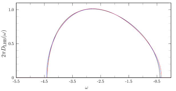
Figure 2: Density of states of the lower Hubbard band, $\pi D_{\rm LHB}^{[n]}(\omega)$ for $U=5$ (bandwidth $W=4$) up to and including orders $n=1,2,3$ (black, blue, red colors).

In Fig. 2 we show the results for the density of states of the lower Hubbard band for $U=5$ (bandwidth $W=4$) to first, second, and third order in $1/U$. The overall spectra display a redshift of the Hubbard semi-ellipse (10) which describes the density of states to leading-order, $2D_{\rm LHB}^{(0)}(\omega)=\rho(\omega+U/2)$. The spectra to higher orders differ from each other mostly by a shift in the spectral support so that the deviations are best visible close to the band edges.

V.1.4 Band part of the Green function

The full solution (V.1.3) contains higher-order corrections in $1/U$ due to the interaction-dependence of the denominator $N(\omega)$. We may expand it order-by-order to derive a Taylor series in $1/U$ for the Green function. Such an order-by-order expansion ignores the fact that the attractive potential $\hat{W}$ generates resonance-contributions at the band edges of the Hubbard band; see below. Therefore, we denote the Green function from the order-by-order expansion as ‘band-part’ Green function. It can be cast into the form

$$2\bar{t}G_{\rm LHB}^{\rm band}(\omega) = \sum_{n=0}^{3}\lambda_{n}(\widetilde{g}_{n}(x)+g_{n}(x))\;,$$

$$2\left(1+\frac{3}{8U^{2}}\right)x = \omega+\frac{U}{2}-\frac{1}{2U}-\frac{35}{8U^{3}}\;,$$

$$\widetilde{g}_{n}(x) = \Theta\left(x^{2}-1\right)\left(T_{n+1}(x)-{\rm sgn}(x)\sqrt{x^{2}-1}U_{n}(x)\right)\;,$$

$$g_{n}(x) = \Theta\left(1-x^{2}\right)\left(T_{n+1}(x)+{\rm i}\sqrt{1-x^{2}}U_{n}(x)\right)\;,$$ (121)

with $T_{n}(x)$ [$U_{n}(x)$] as the Chebyshev polynomials of the first [second] kind Abramovitz and

$$\lambda_{0}=1 \lambda_{1}=-\frac{1}{2U}-\frac{39}{16U^{3}}\;,$$ ,

$$\lambda_{2}=-\frac{1}{4U^{2}} \lambda_{3}=-\frac{1}{8U^{3}}$$ , (122)

are the expansion coefficients. The first-order result was derived earlier in Ref. [Nahrgang, ]. Using an intuitive method, Eastwood et al. kalinowski derived the ‘band-part’ Green function to second order in $1/U$ for the Hubbard model in infinite dimensions. So far, their method could not be extended systematically to higher orders.

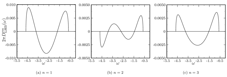
Figure 3: Resonance contribution to the density of states of the lower Hubbard band, $D_{\rm LHB}^{\rm res}(\omega)=D_{\rm LHB}(\omega)-D_{\rm LHB}^{\rm band}(\omega)$, as a function of frequency in $n$th order perturbation theory for $U=5.5$ (bandwidth $W=4$).

In Fig. 3 we show the resonance contribution to the density of states, $D_{{\rm LHB}}^{\rm res}(\omega)$ for $U=5.5$. It is defined as the difference between the band part (121), $D_{\rm LHB}^{\rm band}(\omega)$, and the full density of states $D_{\rm LHB}(\omega)$ (119). The difference is seen to be fairly small which had to be expected because the potential $\hat{W}$ is rather weak. In general, the resonance contributions increase slightly the density of states close to the band edges and decrease it in the middle of the band.

V.2 Comparison with numerical results

Finally, we compare our analytical results with data of advanced numerical methods for the DMFT for the Mott–Hubbard insulator. The Dynamical Density-Matrix Renormalization Group (DDMRG) method provides the gap and the density of states at zero temperature. Nishimoto Quantum Monte-Carlo (QMC) gives the Matsubara Green function at low but finite temperatures. Ref. [kalinowski, ] contains a comparison with early methods in the field.

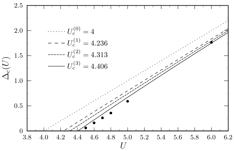
Figure 4: Charge gap as a function of the interaction strength for various orders in the $1/U$-expansion. The dots are DDMRG data points. Nishimoto

V.2.1 Gap

In Fig. 4 we show the gap as a function of the interaction strength for various orders in the $1/U$-expansion together with the DDMRG data of Ref. [Nishimoto, ]. The third-order theory reproduces the DDMRG data points very well.

Note, however, that in another DDMRG study Uhrig the gap closes around $U=4.8$. The differences in the two approaches lies in the reconstruction of the density of states and the extrapolation of the gap from the finite-size data. Apparently, different reconstruction algorithms can result in substantially different extrapolations close to the transition.

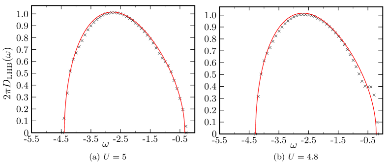
Figure 5: Density of states of the lower Hubbard band from third-order perturbation theory in $1/U$ (full line) in comparison with DDMRG data points Nishimoto for $U=5$ and $U=4.8$.

V.2.2 Lower Hubbard band

In Fig. 5 we show the density of states for $U=4.8$ to third order in $1/U$ together with the DDMRG data of Ref. [Nishimoto, ]. The overall agreement is very good. This has already been observed from the results to second order. kalinowski

It is seen, though, that a resonance develops at the upper band edge in the DDMRG data which is not seen in perturbation theory to third order. For $U=4.5$, the resonance is more pronounced Nishimoto and resembles the split quasi-particle peak of the metallic phase. One may wonder whether such a resonance could be obtained from higher-order perturbation theory. A model study Hoyer shows that the parameter set $\varepsilon_{0}^{*}=-0.2$ and $\varepsilon_{1\leq m\leq 9}^{*}=0.1/m$ in the scattering potential $\hat{W}$ can readily account for both the overall redshift of the density of states and a resonance at the upper band edge. Since the range of the repulsive potential is finite, an expansion of the density of states to high but finite order could possibly reproduce the resonance seen in the DDMRG data.

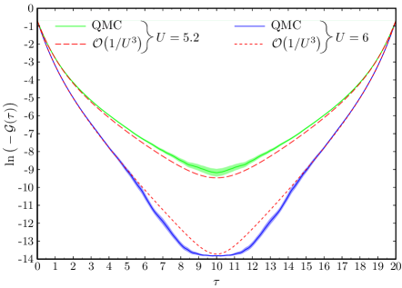
Figure 6: Third-order result and QMC data for the Matsubara Green function for $U=6$ (blue) and $U=5.2$ (green). The inverse temperature is $\beta=20$ ($T=0.05$), the gaps are $\Delta_{\rm c}(U=6)=1.75$ and $\Delta_{\rm c}(U=5.2)=0.89$, respectively. Note that the data are shown on a logarithmic scale. The shading indicates the statistical error in the QMC data.

V.2.3 Matsubara Green function

The Matsubara Green function for the Hubbard model is defined by

$${\cal G}(\tau)=-\frac{1}{L}\sum_{i}{\rm Tr}\left[e^{\beta(\Omega-\hat{H})}{\cal T}_{\tau}\hat{c}_{i,\sigma}(\tau)\hat{c}_{i,\sigma}^{+}(0)\right]\;,$$ (123)

where $\beta=1/k_{\rm B}T$ is the inverse temperature, $\Omega$ is the grand-canonical potential, and ${\cal T}_{\tau}$ orders the operators in imaginary time. The operators in imaginary-time Heisenberg representation are defined by ($-\beta\leq\tau\leq\beta$)

$$\hat{c}_{i,\sigma}(\tau)=e^{\tau\hat{H}}\hat{c}_{i,\sigma}e^{-\tau\hat{H}}\quad,\quad\hat{c}_{i,\sigma}^{+}(\tau)=e^{\tau\hat{H}}\hat{c}_{i,\sigma}^{+}e^{-\tau\hat{H}}\;.$$ (124)

The Fourier transformation of the Matsubara Green function is defined on the points ${\rm i}\omega_{n}=(2n+1)\pi/\beta$ ($n$: integer) on the imaginary axis.

The retarded Green function at finite temperature $T$ is obtained from the analytic continuation,

$$G_{\rm ret}(\omega;\beta)={\cal G}({\rm i}\omega_{n}\to\omega+{\rm i}\eta)\;.$$ (125)

Therefore, we may express the Matsubara Green function with the help of the density of states at finite temperature in the form

$${\cal G}(\tau)=\int_{-\infty}^{\infty}{\rm d}\omega\left[\frac{{\rm Im}\left[G_{\rm ret}(\omega;\beta)\right]}{\pi}\right]\frac{e^{-\omega\tau}}{e^{-\beta\omega}+1}$$ (126)

with $0\leq\tau\leq\beta$. Note that it is easy to evaluate (126) for a given density of states but it is very difficult to reconstruct the density of states from numerical data for ${\cal G}(\tau)$.

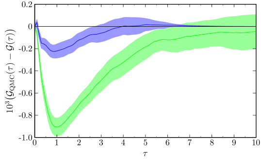
Figure 7: Difference between the third-order result and QMC data for the Matsubara Green function for $U=6$ (blue) and $U=5.2$ (green). The inverse temperature is $\beta=20$ ($T=0.05$), the gaps are $\Delta_{\rm c}(U=6)=1.75$ and $\Delta_{\rm c}(U=5.2)=0.89$, respectively. Note that the difference is augmented by a factor of $10^{3}$ to make it visible. The shading indicates the statistical error in the QMC data.

For very low temperatures and for large interaction strengths we approximate the density of states by its zero-temperature expression to third order,

$${\cal G}(\tau)=-\int_{-\infty}^{\infty}{\rm d}\omega\Bigl{[}D_{\rm LHB}(\omega)+D_{\rm LHB}(-\omega)\Bigr{]}\frac{e^{-\omega\tau}}{e^{-\beta\omega}+1}$$ (127)

which we compare with QMC data of N. Blümer. nils The approximation is not as drastic as it may seem because, deep in the Mott–Hubbard insulator, thermal excitations are exponentially suppressed due to the finite charge gap. Therefore, corrections to (127) should be exponentially small in $\Delta_{\rm c}(U)/k_{\rm B}T$.

In Figs. 6 and 7 we compare our analytical results (127) to QMC data for $\beta=20$ ($T=0.05$) at $U=6$ and $U=5.2$ where the gaps are $\Delta_{\rm c}(U=6)=1.75$ and $\Delta_{\rm c}(U=5.2)=0.89$, respectively. The results agree very well. Note, however, that ${\cal G}(\tau)$ is rather feature-less so that fine points such as the width of the Hubbard bands or the density of states cannot be reconstructed easily from QMC data for ${\cal G}(\tau)$.

VI Conclusions

In this work, we have studied the Mott–Hubbard insulating phase of the Hubbard model on a Bethe lattice with infinite coordination number. We have adopted the Kato–Takahashi perturbation theory to solve the self-consistency equation of the Dynamical Mean-Field Theory for the symmetric single-impurity Anderson model in perturbation theory up to and including third order in the inverse coupling strength $U$. To this end it has been necessary to use the mapping of the single-impurity Anderson model from the ‘star geometry’ onto the ‘two-chain geometry’ which represents the energetically separated lower and upper Hubbard bands. In higher orders, a multi-chain mapping is required in order to resolve the various Hubbard sub-bands. For the present study, we could ignore the secondary Hubbard bands whose weight is of fourth order in $1/U$.

Our results for the Mott–Hubbard gap reproduce those of an earlier analytic study kalinowski of the Hubbard model on the Bethe lattice with infinite coordination number. We confirm the second-order results of Ref. [kalinowski, ] and extend them to third order systematically. The agreement between the perturbation theory in $1/U$ and the DDMRG data of Ref. [Nishimoto, ] for the gap is very good. Note, however, that the precise value of the critical interaction $U_{\rm c}$ where the gap closes, and the analytical behavior of the gap as a function of $U$ close to the transition are still under debate. Uhrig

The previous study kalinowski provides the Green function as a Taylor expansion in $1/U$ whereas the present study includes resonance corrections. The full density of states results from the calculation of the boundary Green function for a particle on a semi-infinite chain with nearest-neighbor electron transfers and an attractive interaction at and near the boundary, whose parameters we derived to third order in $1/U$. For all interaction strengths where perturbation theory is applicable, $U\gtrsim 5$ (bandwidth: $W=4$, $4.4\lesssim U_{\rm c}\lesssim 4.8$), the resonance contributions are small.

For $U\gtrsim 5$, the agreement between the analytical results for the density of states and the DDMRG data Nishimoto is very good for all frequencies. In addition, our zero-temperature expressions for the density of states provides a very good approximation for the density of states at small but finite temperatures. This can be seen from the excellent agreement between our approximate Matsubara Green function and Quantum Monte-Carlo data. nils

As in all kinds of perturbation theories, the number of terms to be calculated rapidly increases with the index of the order. In principle, the fourth-order terms could still be calculated ‘by hand’. This requires a four-chain geometry so that the secondary Hubbard sub-bands can be treated properly. To fourth order there are more than 30 terms in the Kato–Takahashi operator and in the projected Hamiltonian. According to our analysis, much higher orders are needed to reproduce a resonance feature seen in the DDMRG data Nishimoto at the upper band edge of the lower Hubbard band. Such high-order calculations for the density of states appear to be forbiddingly costly within the DMFT.

The ground-state energy of the Hubbard model on the Bethe lattice with infinite coordination number was calculated to high orders using a computer algorithm based on the Kato–Takahashi expansion. eva In the future, we plan to devise a similar algorithm for the calculation of the Mott–Hubbard gap. With a high-order expansion for the Mott–Hubbard gap we should be able to locate $U_{\rm c}$ with a much better accuracy.

Acknowledgments

We thank Marlene Nahrgang for her contributions to the early stages of this work, and Jörg Bünemann for useful discussions.

Appendix A Weight of the secondary lower Hubbard band

We apply particle-hole symmetry and the self-consistency equation (20) to the sum rule for the density of states FetterWalecka and find

$$\frac{1}{2}=\frac{1}{\pi}\int_{-\infty}^{0}{\rm d}\omega{\rm Im}\left[\Delta(\omega)\right]=\sum_{i=0}^{\infty}\biggl{[}\sum_{m}V_{i,m}^{2}\biggr{]}=\sum_{i=0}^{\infty}g_{i}\;,$$ (128)

where we use eq. (57) in the second step. The $i$th sub-band of the Hubbard band contributes the weight $g_{i}$.

The weights $g_{i}$ can be calculated perturbatively. From the definition of the Green function of the lower Hubbard band (39) we can readily write the sum rule (128) as

$$\frac{1}{2}=\frac{1}{\pi}\int_{-\infty}^{0}{\rm d}\omega{\rm Im}\left[G_{\rm LHB}(\omega)\right]=\langle\Phi|\hat{\Gamma}_{0,L}^{+}\hat{d}_{\uparrow}^{+}\hat{d}_{\uparrow}\hat{\Gamma}_{0,L}|\Phi\rangle\;.$$ (129)

The state $|\overline{\Psi}\rangle=\hat{d}_{\uparrow}\hat{\Gamma}_{0,L}|\Phi\rangle$ can readily be calculated from the series expansion of the operator $\hat{\Gamma}_{0,L}$, eq. (34), applied to the state $|\Phi\rangle$, see eqs. (36)-(38). Up to and including third order in $1/U$, we find

$$\hat{P}_{0,L-1}^{(0)}|\overline{\Psi}\rangle=\left(1-\frac{1}{2U^{2}}\right)|\phi_{-1}\rangle-\frac{1}{U}\left(1+\frac{1}{U^{2}}\right)|m_{0;u}\rangle+\frac{1}{U^{2}}|m_{1;u}\rangle-\frac{1}{U^{3}}|m_{2;u}\rangle$$ (130)

in the subspace of the ground-states of $\hat{H}_{0}$ for $L-1$ particles on $L$ lattice sites. In addition, there is a finite second-order contribution in the subspace with excitation energy $U$ above the ground states of $\hat{H}_{0}$,

$$\hat{P}_{1,L-1}^{(0)}|\overline{\Psi}\rangle=\frac{1}{U^{2}}\left(\frac{1}{2}|\phi_{0;u}^{*}\rangle+\frac{1}{2}|\phi_{0;d}^{*}\rangle+|\chi_{0}^{*}\rangle\right)+{\cal O}\left(\frac{1}{U^{3}}\right)\;,$$ (131)

where

$$|\phi_{0;u}^{*}\rangle = \sqrt{\frac{1}{2}}\hat{\beta}_{0,\downarrow}^{+}\hat{\alpha}_{0,\downarrow}\prod_{l=0}^{(L-3)/2}\hat{\alpha}_{l,\uparrow}^{+}\hat{\alpha}_{l,\downarrow}^{+}|\hbox{vac}\rangle\;,$$

$$|\phi_{0;d}^{*}\rangle = -\sqrt{\frac{1}{2}}\hat{\beta}_{0,\uparrow}^{+}\hat{\alpha}_{0,\uparrow}\prod_{l=0}^{(L-3)/2}\hat{\alpha}_{l,\uparrow}^{+}\hat{\alpha}_{l,\downarrow}^{+}|\hbox{vac}\rangle\;,$$ (132)

$$|\chi_{0}^{*}\rangle = -\sqrt{\frac{1}{2}}\hat{\beta}_{0,\downarrow}^{+}\hat{\alpha}_{0,\uparrow}\prod_{l=0}^{(L-3)/2}\hat{\alpha}_{l,\uparrow}^{+}\hat{\alpha}_{l,\downarrow}^{+}|\hbox{vac}\rangle\;.$$

Therefore, the weight of the secondary sub-band, $i=1$, is given by

$$g_{1}=\langle\overline{\Psi}|\hat{P}_{1,L-1}^{(0)}|\overline{\Psi}\rangle=\frac{1}{2U^{4}}\left(\frac{1}{4}+\frac{1}{4}+1\right)=\frac{3}{4U^{4}}\;,$$ (133)

and corrections are of higher order in $1/U$. Because the higher sub-bands are even smaller in weight, $g_{i\geq 2}={\cal O}(U^{-5})$, we can conclude from the sum-rule that $g_{0}=1/2-3/(4U^{4})$. The direct calculation of $g_{0}$ from eq. (130) is not possible because it lacks the fourth-order correction $-7/(4U^{4})|\phi_{-1}\rangle$.

Equation (133) shows that, up to and including third order in $1/U$, only the primary Hubbard sub-band contributes to the density of states for $\omega<0$.

Appendix B Green functions for a semi-infinite tight-binding chain

Let $\hat{B}=\sum_{l=0}^{\infty}|l\rangle\langle l+1|+|l+1\rangle\langle l|$ describe the motion of a single particle over a semi-infinite chain. By definition, we have $\hat{B}|0\rangle=|1\rangle$ and $\hat{B}|l\rangle=|l+1\rangle+|l-1\rangle$ for $l\geq 1$. By induction we can prove the following lemma:

• For all $n\in\mathbb{N}_{0}$ we find

  $$U_{n}(\hat{B}/2)|0\rangle=|n\rangle\;.$$ (134)

  Here, $U(x)$ are the Chebyshev polynomials of the second kind. Abramovitz

• For all $n,l\in\mathbb{N}$ we have

  $$U_{n}(\hat{B}/2)|l\rangle=\sum_{i=0}^{n}\Theta_{2(l-n)+2i}|l-n+2i\rangle\;.$$ (135)

  Here, $\Theta_{l}$ denotes the discrete unit-step function $\Theta:\mathbb{Z}\rightarrow\{0,1\}$,

  $$\Theta_{l}:=\left\{\begin{array}[]{rll}1&\hbox{for}&l\geq 0\;,\\ 0&\hbox{for}&l<0\;.\end{array}\right.$$ (136)

For the imaginary part of the bare Green function (114) we can write ($\widetilde{\omega}=\omega+U/2-\bar{\varepsilon}$)

$${\rm Im}\left[g_{l,m}^{(0)}(\omega)\right]=\pi\langle l|\delta\left(\widetilde{\omega}\openone-\bar{t}\hat{B}\right)|m\rangle\;,$$ (137)

which is finite in the interval $|\widetilde{\omega}|\leq 2\bar{t}$. We set $x=\widetilde{\omega}/(2\bar{t})$ and obtain

$${\rm Im}\left[g_{l,m}^{(0)}(\omega)\right]=\frac{\pi}{2\bar{t}}\langle l|\delta\left(x\openone-\hat{B}/2\right)|m\rangle\;.$$ (138)

When we formally expand the ‘function’ $f(x)=\pi\delta(x-z)$ ($|x|\leq 1$, $|z|\leq 1$) in a Chebyshev series, ruhl

$$\pi\delta(x-z)=2\sqrt{1-x^{2}}\sum_{n=0}^{\infty}U_{n}(x)U_{n}(z)\;,$$ (139)

we can write the imaginary part of the bare Green function as

$${\rm Im}\left[g_{l,m}^{(0)}(\omega)\right]=\frac{1}{\bar{t}}\Theta\left(1-x^{2}\right)\sqrt{1-x^{2}}\sum_{n=0}^{\infty}U_{n}(x)\langle l|U_{n}(\hat{B}/2)|m\rangle\;.$$ (140)

Because $\hat{B}$ is Hermitian so that $g_{l,m}^{(0)}(\omega)=g_{m,l}^{(0)}(\omega)$, we can restrict ourselves to $l=m+h$ with $h\in\mathbb{N}_{0}$. With the help of the lemma, it is not difficult to show that for $h,m\in\mathbb{N}_{0}$,

$$\bar{t}{\rm Im}\left[g_{m+h,m}^{(0)}(\omega)\right] = \Theta(1-x^{2})\sqrt{1-x^{2}}\Bigl{\{}\delta_{m,0}U_{h}(x)$$ (141)

$$+(1-\delta_{m,0})\sum_{k,y=0}^{\infty}\Theta_{m+y-k}\Theta_{k-y}\left[U_{2k}(x)\delta_{h,2y}+U_{2k+1}(x)\delta_{h,2y+1}\right]\Bigr{\}}$$

with the abbreviation $x=(\omega+U/2-\bar{\varepsilon})/(2\bar{t})$, the discrete unit-step function $\Theta_{l}$, see (136), and $\Theta(x)$ as the Heaviside step-function.

The real part follows from the Kramers–Kronig transformation. FetterWalecka We find ruhl

$$\bar{t}{\rm Re}\left[g_{m+h,m}^{(0)}(\omega)\right]=\delta_{m,0}I_{h}(x)+(1-\delta_{m,0})\sum_{k,y=0}^{\infty}\Theta_{m+y-k}\Theta_{k-y}\left[I_{2k}(x)\delta_{h,2y}+I_{2k+1}(x)\delta_{h,2y+1}\right]\;.$$ (142)

As is proven by induction in Ref. [ruhl, ], we have ($n\in\mathbb{N}_{0},p\in\mathbb{N}$),

$$I_{n}(x) = T_{n+1}(x)\quad\hbox{for}\quad|x|\leq 1\;,$$

$$I_{n}(x) = T_{n+1}(x)-{\rm sgn}(x)\sqrt{x^{2}-1}U_{n}(x)\quad\hbox{for}\quad|x|\geq 1\;,$$ (143)

$${}[I_{n}(x)]^{p} = T_{p(n+1)}(x)-{\rm sgn}(x)\sqrt{x^{2}-1}U_{p(n+1)-1}(x)\quad\hbox{for}\quad|x|\geq 1\;,$$

where $T_{n}(x)$ are the Chebyshev polynomials of the first kind. Abramovitz In particular, the bare boundary Green function reads ($\omega<0$)

$$\bar{t}g_{0,0}^{(0)}(\omega)=\Theta\left(x^{2}-1\right)\left(x-{\rm sgn}(x)\sqrt{x^{2}-1}\right)+\Theta\left(1-x^{2}\right)\left[x+{\rm i}\sqrt{1-x^{2}}\right]\;.$$ (144)

Finally, we note that powers of the bare Green function obey for $n\in\mathbb{N}_{0},p\in\mathbb{N}$

$$\bar{t}^{p}g_{n,0}^{p}(\omega)=\Theta(x^{2}-1)I_{n}^{p}(x)+\Theta(1-x^{2})\left\{T_{p(n+1)}(x)+{\rm i}\sqrt{1-x^{2}}U_{p(n+1)-1}(x)\right\}\;.$$ (145)

With these relations and the properties of the Chebyshev polynomials, one can readily prove eq. (118); for details, see Ref. [ruhl, ].

References

• (1) A. Georges, G. Kotliar, W. Krauth, and M.J. Rozenberg, Rev. Mod. Phys. 68, 13 (1996).
• (2) W. Metzner and D. Vollhardt, Phys. Rev. Lett. 62, 324 (1989).
• (3) R. Bulla, Phys. Rev. Lett. 83, 136 (1999); for a review on the method, see R. Bulla, T. Costi, and Th. Pruschke, Rev. Mod. Phys. 80, 395 (2008).
• (4) M. Caffarel and W. Krauth, Phys. Rev. Lett. 72, 1545 (1994); Y. $\bar{\rm O}$no, R. Bulla, A.C. Hewson, and M. Potthoff, Eur. Phys. J. B 22, 283 (2001).
• (5) Q. Si, M.J. Rozenberg, G. Kotliar, and A.E. Ruckenstein, Phys. Rev. Lett. 72, 2761 (1994).
• (6) M.P. Eastwood, F. Gebhard, E. Kalinowski, S. Nishimoto, and R.M. Noack, Eur. Phys. J. B 35, 155 (2003).
• (7) R.M. Noack and F. Gebhard, Phys. Rev. Lett. 82, 1915 (1999); S. Ejima, F. Gebhard, and R.M. Noack, Eur. Phys. J. B 66, 191 (2008).
• (8) S. Nishimoto, F. Gebhard, and E. Jeckelmann, J. Phys.: Condens. Matter 16, 7063 (2004).
• (9) M. Karski, C. Raas, and G.S. Uhrig, Phys. Rev. B 72, 113110 (2005).
• (10) M. Jarrell, Phys. Rev. Lett. 69, 168 (1992).
• (11) N. Blümer, Phys. Rev. B 76, 205120 (2007).
• (12) A.N. Rubtsov, V.V. Savkin, and A.I. Lichtenstein, Phys. Rev. B 72, 035122 (2005); P. Werner, A. Comanac, L. de Medici, M. Troyer, and A.J. Millis, Phys. Rev. Lett. 97, 076405 (2006).
• (13) M.J. Rozenberg, G. Kotliar, and X.Y. Zhang, Phys. Rev. B 49, 10181 (1994).
• (14) D.E. Logan, M.P. Eastwood, and M.A. Tusch, J. Phys.: Condens. Matt. 9 4211 (1997).
• (15) M. Potthoff, Eur. Phys. J B 36, 335 (2003).
• (16) F. Gebhard, E. Jeckelmann, S. Mahlert, S. Nishimoto, and R.M. Noack, Eur. Phys. J. B 36, 491 (2003).
• (17) D. Ruhl and F. Gebhard, J. Stat. Mech. Exp. Theor. P03015 (2006).
• (18) T. Kato, Prog. Theor. Phys. 4, 514 (1949).
• (19) M. Takahashi, J. Phys. C 10, 1289 (1977).
• (20) D. Ruhl, PhD thesis (unpublished; Marburg, 2010); available electronically as http://archiv. ub.uni-marburg.de/diss/z2010/0377/pdf/ddfr.pdf
• (21) R.J. Baxter, Exactly Solved Models in Statistical Mechanics (Dover Publications, New York, 2007).
• (22) A.L. Fetter and J.D. Walecka, Quantum Theory of Many-Particle Systems, (Dover Publications, New York, 2003).
• (23) M. Eckstein, M. Kollar, K. Byczuk, and D. Vollhardt, Phys. Rev. B 71, 235119 (2005).
• (24) For a review, see A.C. Hewson, The Kondo problem to heavy fermions (Cambridge University Press, Cambridge, 1993).
• (25) D.E. Logan, M.P. Eastwood, and M.A. Tusch, J. Phys.: Condens. Matter 10, 2673 (1998); M.R. Galpin and D.E. Logan, Eur. Phys. J. B 62, 129 (2008).
• (26) E.H. Lieb and F.Y. Wu, Phys. Rev. Lett. 20, 1445 (1968).
• (27) N.F. Mott, Metal-insulator transitions (Taylor and Francis, London, 1974, 1990); F. Gebhard, The Mott Metal-Insulator Transition (Springer, Berlin, 1997).
• (28) For a first application of this idea, see M. Nahrgang, diploma thesis (unpublished; Marburg, 2008).
• (29) M.J. Rozenberg, G. Möller, and G. Kotliar, Mod. Phys. Lett. 8, 535 (1994).
• (30) W. Metzner, P. Schmit, and D. Vollhardt, Phys. Rev. B 45, 2237 (1992).
• (31) E.N. Economou, Green’s Functions in Quantum Physics (Springer Series in Solid-State Sciences 7, Springer, Berlin, 1979), chap. 6.
• (32) M. Hoyer, B.Sc. thesis (Marburg, 2010; unpublished).
• (33) M. Abramovitz and I.A. Stegun, Handbook of Mathematical Functions (Dover Publications, New York, 1970).
• (34) N. Blümer (private communication, 2010).
• (35) N. Blümer and E. Kalinowski, Phys. Rev. B 71, 195102 (2005).