Quantum phase diagram of the half filled Hubbard model with bond-charge interaction.

Abstract

Using quantum field theory and bosonization, we determine the quantum phase diagram of the one-dimensional Hubbard model with bond-charge interaction $X$ in addition to the usual Coulomb repulsion $U$ at half-filling, for small values of the interactions. We show that it is essential to take into account formally irrelevant terms of order $X$. They generate relevant terms proportional to $X^{2}$ in the flow of the renormalization group (RG). These terms are calculated using operator product expansions. The model shows three phases separated by a charge transition at $U=U_{c}$ and a spin transition at $U=U_{s}>U_{c}$. For $U<U_{c}$ singlet superconducting correlations dominate, while for $U>U_{s}$, the system is in the spin-density wave phase as in the usual Hubbard model. For intermediate values $U_{c}<U<U_{s}$, the system is in a spontaneously dimerized bond-ordered wave phase, which is absent in the ordinary Hubbard model with $X=0$. We obtain that the charge transition remains at $U_{c}=0$ for $X\neq 0$. Solving the RG equations for the spin sector, we provide an analytical expression for $U_{s}(X)$. The results, with only one adjustable parameter, are in excellent agreement with numerical ones for $X<t/2$ where $t$ is the hopping.

, ,

1 Introduction

1.1 The model

The Hubbard model, with nearest-neighbor hopping $t$ and on-site repulsion $U$ has been widely used to study the effects of correlations, as a simplified model to describe compounds of transition metals and other systems. However, one expects that in any system, in general the hopping between two sites depend on the occupation of these two sites, which leads to the presence of bond-charge interactions (also called correlated hopping terms) in the Hamiltonian [such as $X$ in Eq. (1) and $\sum_{\sigma,\langle ij\rangle}(c_{i\sigma}^{\dagger}c_{j\sigma}+{\rm H.c.})n_{i-\sigma}n_{j-\sigma}$]. For example, in simple systems with one relevant orbital per site, one would expect that when electrons are added to one site, the screening of the core charge increases, and as a consequence, the wave function of the orbital expands and the hopping to the nearest sites increases. In general, any one-band effective model derived from more complex Hamiltonians to describe the low-energy physics of some system, contains bond-charge interactions. In fact, the generalized Hubbard model with correlated hopping terms has been derived and used to describe the low-energy physics of intermediate valence systems [1], organic compounds [2, 3, 4, 5, 6, 7], a Hubbard model including lattice vibrations [8], cuprate superconductors [9, 10, 11], and more recently optical lattices [12, 13, 14]. This is particularly interesting because the parameters can be tuned experimentally in a wide range [14, 15]. First-principles calculations in transition-metal complexes suggest that the correlated hopping terms can be large [16].

As we shall see, the presence of bond-charge interaction leads to qualitatively new physics. One example is that in two dimensions $d$-wave pairing correlations, which are already present in the Hubbard model [17] are strongly enhanced in the generalized Hubbard model for the cuprates [18], and one obtains $d$-wave superconductivity already at the mean-field level [19]. In one dimension (1D), field-theoretical [20, 21] and numerical [21, 22] results show the presence of a spontaneously dimerized bond-ordering wave (BOW) and a phase with dominant triplet superconducting correlations at large distances that are absent in the ordinary Hubbard model. For special values of the parameters, the model with two- and three-body interactions has been solved exactly by the Bethe ansatz [23].

The simplest model with bond-charge interaction has been proposed by Hirsch motivated by his theory of hole superconductivity [24, 25]. The Hamiltonian can be written as

$$H=-t\sum_{\sigma=\uparrow,\downarrow,\langle ij\rangle}(c_{i\sigma}^{\dagger}c_{j\sigma}+{\rm H.c.})+U\sum_{i}n_{i\uparrow}n_{i\downarrow}+X\sum_{\sigma,\langle ij\rangle}(c_{i\sigma}^{\dagger}c_{j\sigma}+{\rm H.c.})(n_{i-\sigma}+n_{j-\sigma}).$$ (1)

In 1D, the model can display a phase with dominant singlet superconducting (SS) correlations, even for positive $U$ [21, 26, 27, 28]. For $X=t$, the model has been solved exactly and there is a metal-insulator transition for increasing $U$ [29, 30, 31]. More recently, the role of entanglement in this quantum phase transition has been studied [32, 33]. The response of the system to an applied magnetic flux indicates that the metallic phase is not superconducting [31]. However, the ground state is highly degenerate in this phase at it is difficult to predict from the exact solution what happens when the degeneracy is lifted by a small but finite $X-t$. In any case, standard bosonization [20, 21, 26] and numerical studies [27] have provided a general physical picture of the behavior of the model, except at half filling. In this case, taking as usual only the leading terms in the lattice constant $a$, $X$ disappears in the bosonization treatment [it enters as $X\cos(\nu\pi)$, where $\nu$ is the filling fraction [26, 21]]. Therefore, standard field theory predicts a SS phase for $U<0$, and a spin-density wave (SDW) phase for $U>0$, as in the usual Hubbard model. However, a charge insulator-metal transition driven by $X$ at finite $U_{c}>0$ has been found numerically [34] and later a quantum phase diagram has been derived which includes a BOW phase [35]. Recently, new numerical studies of the model at arbitrary filling identify regions of phase separation for $X>0.5t$ [36].

1.2 Phase diagram at half filling

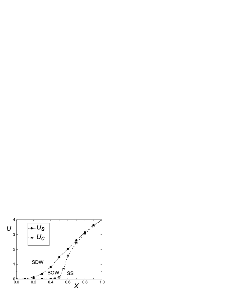
Figure 1: Phase diagram of the model at half filling obtained from the method of level crossings. Squares: charge transition. Solid circles: spin transition. The unit of energy is taken as $t=1$.

The quantum phase diagram for $\nu=1/2$ has been obtained by a combination of different numerical techniques [35, 36]. In Fig. 1 we reproduce the phase diagram obtained by the method of topological transitions [22, 37]. These transitions correspond to jumps in the charge and spin Berry phases which signal the corresponding transitions between the thermodynamic phases, and coincide with a corresponding crossing of excited levels, justified on the basis of conformal-field theory [37, 38]. These quantities are also related to charge and spin localization indicators [39, 40, 41, 42] used for example to characterize valence-bond-solid states in quantum spin chains [43]. While changes in the Berry phase are proportional to changes in polarization, the spin Berry phase tensor provides a geometric characterization of the ferrotoroidic moment [42].

The critical values of $U$ for the charge ($U_{c}$) and spin ($U_{s}$) transition have been calculated in systems of up to $L=14$ lattice sites, and extrapolated to the thermodynamic limit using a parabola in $1/L^{2}$. Fig. 1 displays the extrapolated values for $0\leqslant X\leqslant 1$. It is important to note that this interval can be extended to the whole real axis using symmetry properties of the Hamiltonian [27]. A change of phase of half of the sites [$c_{i\sigma}^{\dagger}\rightarrow(-1)^{i}c_{i\sigma}^{\dagger}$], interchanges the signs of $t$ and $X$, so that $H(-t,-X,U)\equiv H(t,X,U)$. Combining this with an electron-hole transformation ($c_{i\sigma}^{\dagger}\rightarrow c_{i\sigma}$), one obtains at half filling

$$H(t-2X,-X,U)\equiv H(t,X,U)\equiv H(2X-t,X,U).$$ (2)

Then, if the critical ratio $u(x)$ ($U_{c}/t$ or $U_{s}/t$) with $x=X/t$, $t>0$, is known in the interval $0\leqslant x<1/2$, it can be extended to negative values of $X$ using the first Eq. (2). Similarly, the second Eq. (2) maps the interval $1/2<x\leqslant 1$ onto $x\eqslantgtr 1$. Explicitly

$${\rm if}x<0{\rm,\;}u(x)=(1-2x)u\left(\frac{-x}{1-2x}\right){\rm;\;if}x\eqslantgtr 1{\rm,\;}u(x)=(2x-1)u\left(\frac{x}{2x-1}\right).$$ (3)

It is interesting to note that the end points $x\rightarrow\pm\infty$ are mapped onto $x=1/2.$

For $U>U_{c}$ ($U<U_{s}$), the system has a charge (spin) gap. For $U<U_{c}$, the system is in the SS phase, while for $U>U_{s}$, the system is in the SDW phase, according to the dominant correlation functions at large distances. In between, for $U_{c}<U<U_{s}$, one has the fully gapped BOW phase. For small values of the interactions, the dominant correlation functions in each phase can be understood from field theory [20, 21]. For $X>t/2$, the SS phase displays incommensurate correlations [35], which can be qualitatively understood using a mean field approximation in one of the terms obtained from bosonization [35], leading to a commensurate-incommensurate transition, with some similarities to the physics of the Hubbard model when a large next-nearest-neighbor hopping is added [44], and some spin systems [45]. The spontaneously dimerized BOW phase has also been also found in the Hubbard model with alternative on-site energies [37, 46, 47, 48, 49, 50, 51, 52, 53], where it displays ferroelectricity [37, 51, 52]. The presence of the BOW phase in this model was first predicted using field theory and bosonization [46, 47].

For $X<t/2$, the numerical results for the charge transition are consistent with $U_{c}=0$, as in the ordinary Hubbard model [35]. The accuracy of the results are not enough to establish if there is a kink or not at $X=t/2$, $U_{c}=0$. Arianna Montorsi has found that a good fit of the numerical results for $t/2\leqslant X\leqslant t$ is [54]

$${\rm if}x\eqslantgtr 1/2{\rm,\;}u_{c}=4\sqrt{2x-1}{\rm,\;}$$ (4)

which is consistent with a kink at $x-1/2=u_{c}=0$, and has the nice property that when it is extended analytically to $x\eqslantgtr 1$, it satisfies the second symmetry relation (3). The value $U_{c}=4t$ for $X=1$, is consistent with the exact solution [29, 30, 31] To our knowledge, no justification of Eq. (4) exists so far.

It has been verified that the spin transition is of Kosterlitz-Thouless type [35]. In contrast to $U_{c}$, the critical value for the spin transition $U_{s}(X)$ represented in Fig. 1 is smooth. For small values of $X$, it increases as $X^{2}$, while for $X\sim t/2$ there is an inflection point. For $X<t$, $U_{s}>U_{c}$. While for $X=t$, $U_{s}=U_{c}=4t$, the second Eq. (3) implies that for $X>t$, also $U_{s}>U_{c}$. Therefore, there is no crossing between $U_{c}(X)$ and $U_{s}(X)$ at $X=t$. The fact that there is a finite value of $U_{s}(1/2)$ and the second Eq. (3) imply that $U_{s}(X)$ grows linearly with $X$ for $X\rightarrow+\infty$, in contrast to the $\sqrt{X}$ behavior for the charge transition predicted by Eq. (4).

1.3 Previous field-theoretical results

As stated in Section 1.1, standard continuum limit field theory and bosonization fails at half filling because $X$ disappears from the $g_{i}$ coupling constants [26, 21]. In Ref. [35] we have calculated vertex corrections to these $g_{i}$ using second order perturbation theory in the bond-charge interaction $X$. The approach is similar to that done by Tsuchiizu and Furusaki for the Hubbard model extended with nearest-neighbor repulsion [56], but for our Hamiltonian, Eq. (1) it is not necessary to introduce a low-energy cutoff. This approach led to the following critical $U$ at the spin transition

$$U_{s}=\frac{8X^{2}}{\pi(t-X)}$$ (5)

This function lies below the numerical points in Fig. 1, but seems to represent correctly the limit $X\rightarrow 0$. However, unfortunately the prediction of this approach for the charge transition is $U_{c}\sim U_{s}/2$ for small $X$, instead of $U_{c}=0$ found numerically. In addition, with vertex corrections only, it is not possible to explain the nature of the incommensurate SS phase for $X>t/2$.

In Ref. [35] we have also considered in the bosonized theory, a term in next to leading order in the lattice parameter $a$, which couples charge and spin in a mean-field approximation. However, this approximation is questionable, and the quantitative agreement between the analytical and numerical results for the charge transition is poor.

In this work we include all terms of next to leading order in $a$, and include them in a renormalization group (RG) treatment. This approach is superior to perturbation theory in $X$ (as included in Ref. [35] through vertex corrections). Retaining all these terms leads to a lengthy algebra, but unfortunately selecting only a few of them, breaks the SU(2) symmetry and leads to wrong results. Since our approach is a weak coupling one, we restrict our study to $X<t/2$, which seems to be the more realistic regime of parameters. Our effort is rewarded by an excellent agreement with the numerical results for both critical values of $U$ at the corresponding transitions.

2 The field-theoretical approach

2.1 The continuum limit

In order to construct the low-energy field theory for the Hamiltonian Eq. (1), we suposse that both $U$ and $X$ are small. Therefore, in the Fourier development of fermion operators we retain only the modes near $-k_{F}$ and $k_{F}$, where $k_{F}$ is the Fermi wave vector. Introducing a cutoff $\Lambda<<1/a$, where $a$ is the lattice parameter, and calling $L$ the lenght of the system, the local annihilation operator $c_{n\sigma}$ can be written as:

$$c_{n\sigma} = \sqrt{\frac{a}{L}}\sum^{\frac{\pi}{a}}_{k=-\frac{\pi}{a}}e^{ikna}c_{k\sigma}$$ (6)

$$\sim \sqrt{\frac{a}{L}}\left[e^{-ik_{F}na}\sum_{-\Lambda<k+k_{F}<\Lambda}e^{i(k+k_{F})na}c_{k\sigma}+e^{ik_{F}na}\sum_{-\Lambda<k-k_{F}<\Lambda}e^{i(k-k_{F})na}c_{k\sigma}\right]\equiv$$

$$\sqrt{a}\left[e^{-ik_{F}n}\psi_{\sigma-}(x=na)+e^{ik_{F}na}\psi_{\sigma+}(x=na)\right]$$

in the last step we have introduced the left and right fermionic fields $\psi_{\sigma-}(x)$ and $\psi_{\sigma+}(x)$ respectively, by replacing the discrete lattice index $n$ by a continuous variable $x\sim na$. This is possible because of the very small change undergone by sums in the second line of the previous equation, when one goes from site $n$ to $n+1$.

Now we can undertake a gradient expansion for $H$ by making the replacement

$$\psi_{\sigma\pm}[x=(n+1)a)]\rightarrow\psi_{\sigma\pm}(x=na)+a\partial_{x}\psi_{\sigma\pm}(x))$$ (7)

in all the terms of Eq. (1). For the hopping operator we obtain

$$(c_{n\sigma}^{\dagger}c_{n+1\sigma}+c_{n+1\sigma}^{\dagger}c_{n\sigma}) \sim 2ia(-1)^{n}(\psi_{\sigma-}^{\dagger}\psi_{\sigma+}-\psi_{\sigma+}^{\dagger}\psi_{\sigma-})+$$ (8)

$$a^{2} i[(\psi_{\sigma+}^{\dagger}\partial_{x}\psi_{\sigma+}-\partial_{x}\psi_{\sigma+}^{\dagger}\psi_{\sigma+}-\psi_{\sigma-}^{\dagger}\partial_{x}\psi_{\sigma-}+\partial_{x}\psi_{\sigma-}^{\dagger}\psi_{\sigma-})+$$

$$(-1)^{n} \partial_{x}(\psi_{\sigma-}^{\dagger}\psi_{\sigma+}-\psi_{\sigma+}^{\dagger}\psi_{\sigma-})]+O(a^{3}),$$

where we have used $k_{F}=\pi/(2a)$. The number operator becomes

$$n_{n{\sigma}} \sim a\bigg{[}\rho_{\sigma+}(x)+\rho_{\sigma-}(x))$$ (9)

$$+ (-1)^{n}\left(\psi_{\sigma+}^{\dagger}(x)\psi_{\sigma-}(x)+\psi_{\sigma-}^{\dagger}(x)\psi_{\sigma+}(x)\right)\bigg{]}$$

with $\rho_{\sigma+}=\psi_{\sigma+}^{\dagger}\psi_{\sigma+}$ and $\rho_{\sigma-}=\psi_{\sigma-}^{\dagger}\psi_{\sigma-}$.

By replacing $\sum_{n}$ by $\int\frac{dx}{a}$ and taking into account that the integration of terms with an oscillating $(-1)^{n}$ prefactor vanish, one obtains for the Hubbard Hamiltonian [corresponding to the first two terms of Eq. (1)] the following form:

$$H_{U} = iv_{F}\int dx\left\{\psi_{\sigma+}^{\dagger}\partial_{x}\psi_{\sigma+}-\partial_{x}\psi_{\sigma+}^{\dagger}\psi_{\sigma+}-\psi_{\sigma-}^{\dagger}\partial_{x}\psi_{\sigma-}+\partial_{x}\psi_{\sigma-}^{\dagger}\psi_{\sigma-}\right\}+$$ (10)

$$\int dx\sum_{\sigma}\bigg{\{}\frac{g_{4\perp}}{2}(\psi^{\dagger}_{\sigma+}\psi_{\sigma+}\psi^{\dagger}_{\overline{\sigma}+}\psi_{\overline{\sigma}+}+\psi^{\dagger}_{\sigma-}\psi_{\sigma-}\psi^{\dagger}_{\overline{\sigma}-}\psi_{\overline{\sigma}-})+g_{2\perp}\psi^{\dagger}_{\sigma+}\psi_{\sigma+}\psi^{\dagger}_{\overline{\sigma}-}\psi_{\overline{\sigma}-}+$$

$$g_{1\perp}\psi^{\dagger}_{\sigma+}\psi_{\sigma-}\psi^{\dagger}_{\overline{\sigma}-}\psi_{\overline{\sigma}+}+\frac{g_{3\perp}}{2}(\psi^{\dagger}_{\sigma-}\psi_{\sigma+}\psi^{\dagger}_{\overline{\sigma}-}\psi_{\overline{\sigma}+}+h.c.)\bigg{\}}.$$

The first line corresponds to the usual free Dirac Hamiltonian with $v_{F}=at$ the bare Fermi velocity (later we shall use $v_{F}=a(t-X)$, the Hartree-Fock value [21]) The terms with prefactors $g_{1\perp}$, $g_{2\perp}$, $g_{3\perp}$, $g_{4\perp}$ correspond to backward, forward two branch, Umklapp and forward one branch, respectively. While all these constants are equal to $aU$, they might run independently under a renormalization group (RG) flow. Moreover, in units in which $\hbar=1$ and $v_{F}=1$, the couplings $g_{i}$ are dimensionless. Now, if a coupling constant $g_{i}$ has units $E^{d-\Delta_{i}}$, $\Delta_{i}$ is known as the scaling dimension of the corresponding operator $O_{i}$, where $d$ is the spacetime dimension ($2$ in our case) [57]. Therefore all interactions in Eq. (10) have scaling dimension $2$, they are marginal operators. It is known that depending on the sign of the $g_{i}$ which correspond to the charge or spin sector of the theory, they can become marginally relevant or irrelevant. The first case leads to a charge or spin gap [58] (see also Section 2.4). Let us see how this situation is modified by inclusion of the correlated hopping term [the last one in Eq. (1)]

The sum of the number operators in (1) has the following gradient expansion:

$$(n_{n\overline{\sigma}}+n_{i+1\overline{\sigma}}) \sim 2a(\rho_{\overline{\sigma}+}+\rho_{\overline{\sigma}-})+a^{2}[\partial_{x}(\rho_{\overline{\sigma}+}+\rho_{\overline{\sigma}-})-$$ (11)

$$(-1)^{n} (\partial_{x}(\psi^{\dagger}_{\overline{\sigma}-}\psi_{\overline{\sigma}+}+\psi^{\dagger}_{\overline{\sigma}+}\psi_{\overline{\sigma}-}))]+O(a^{3})$$

multiplying (8) by (11) we see that the terms quadratic in $a$ are oscillating and vanish under integration. This is the result anticipated in Section 1.1. This means that no scattering $\it at$ the Fermi level is generated by the correlated hopping interaction. We should include term up to $O(a^{2})$ in the Hamiltonian. We obtain:

$$H_{X} = i\int dx\sum_{\sigma}\bigg{\{}g_{4\perp}^{\prime}[-\partial_{x}\psi_{\sigma+}^{\dagger}\psi_{\sigma+}\psi_{\overline{\sigma}+}^{\dagger}\psi_{\overline{\sigma}+}+\partial_{x}\psi_{\sigma-}^{\dagger}\psi_{\sigma-}\psi_{\overline{\sigma}-}^{\dagger}\psi_{\overline{\sigma}-}-{\rm H.c.}]$$ (12)

$$g_{2\perp}^{\prime}[-\partial_{x}\psi_{\sigma+}^{\dagger}\psi_{\sigma+}\psi_{\overline{\sigma}-}^{\dagger}\psi_{\overline{\sigma}-}+\partial_{x}\psi_{\sigma-}^{\dagger}\psi_{\sigma-}\psi_{\overline{\sigma}+}^{\dagger}\psi_{\overline{\sigma}+}-{\rm H.c.}]$$

$$g_{1\perp}^{\prime}[-\partial_{x}\psi_{\sigma+}^{\dagger}\psi_{\sigma-}\psi_{\overline{\sigma}-}^{\dagger}\psi_{\overline{\sigma}+}+\partial_{x}\psi_{\sigma-}^{\dagger}\psi_{\sigma+}\psi_{\overline{\sigma}+}^{\dagger}\psi_{\overline{\sigma}-}-{\rm H.c.}]$$

$$g_{3\perp}^{\prime}[-\partial_{x}\psi_{\sigma-}^{\dagger}\psi_{\sigma+}\psi_{\overline{\sigma}-}^{\dagger}\psi_{\overline{\sigma}+}+\partial_{x}\psi_{\sigma+}^{\dagger}\psi_{\sigma-}\psi_{\overline{\sigma}+}^{\dagger}\psi_{\overline{\sigma}-}-{\rm H.c.}]\bigg{\}}$$

where all $g_{i}^{\prime}=a^{2}X$. The essential differences between the field theory given by Eq. (12) and the one given by Eq. (10) is the non local nature of the interaction arising from the derivatives. In $k$-space this corresponds to scattering of electrons which are near but not $\it on$ the Fermi surface.

Note that the coupling constants $g_{i}^{\prime}$ has dimension of the inverse of energy. Therefore each term of Eq. (12) has dimension 3, they are irrelevant. As only these irrelevant operators appear in the low energy fermionic field theory of the correlated hopping term $H_{X}$, one might be tempted to conclude that there is no contribution of these terms to the physical behavior of the system, in contrast to the numerical results discussed in Section 1.2.  How could we account of this situation with our field theoretical analysis? In fact, from a renormalization group (RG) point of view, all the operators allowed by symmetry should be included in the effective theory. The fact that operators present in Eq. (10) were not obtained in the derivation of Eq. (12) means that in the initial conditions, the different $g$ do not depend on $X$. However, they could acquire an $X$ dependence by the couplings between $g$ and $g^{\prime}$ when the RG flow evolves.

We can take advatage of the well known studies of thermal critical phenomena with RG [59] to further understand this issue. For this case we know that the irrelevance of an operator means that the critical exponents are not affected by its presence in the Hamiltonian. However the critical temperature does depend on this operator. In our case the presence of irrelevant operators will be crucial to determine the boundaries in parameter space of the different phases, where the spin or charge gap opens.

Finally, we note that the SU(2) invariance of the ordinary Hubbard model implies that under RG flow, $g_{2\perp}=g_{1\perp}$ remains [58]. Similarly, it is shown in A that $g_{2\perp}^{\prime}=g_{1\perp}^{\prime}$ is required to keep the SU(2) invariance of the full Hamiltonian.

2.2 Bosonization

Bosonization is a powerful technique to analyze interacting one-dimensional fermionic systems [58]. Some of the interacting terms in the fermionic Hamiltonian become free non-interacting terms in the bosonic Hamiltonian. The remaining terms contain in general cosines of the bosonic fields. Their effect can be studied by a perturbative implementation of the RG method. If in the RG flow the coefficient of a cosine decreases, the fixed point corresponds to a trivial theory of free bosons with known properties. When the RG flow goes to strong coupling the coefficient of a cosine increases. The fields are trapped in a minimum of the free energy and the different phases can be characterized by calculating the classical value at this minimum of the bosonic operators corresponding to the physical observables. In our case, the RG analysis is more involved, but as we shall show, it leads to a tractable theory and correct results.

Let us therefore resort to a bosonic representation of the fermionic theory of Eq. (12) We use the following bosonization formula for the left ($-$) and right ($+$) fermions[60] :

$$\psi_{\sigma\pm}(x) = \frac{F_{\sigma\pm}}{\sqrt{L}}\colon e^{\mp i\phi_{\sigma\pm}}\colon$$ (13)

$$= \frac{F_{\sigma\pm}}{\sqrt{2\pi\alpha}}e^{\mp i\phi_{\sigma\pm}}$$ (14)

Equation (13) is normal ordered and therefore does not contain a somewhat uncomfortable short range cutoff $\alpha$, $F$ is the Klein factor and $L$ the length of the chain. Eq. (14) arises from Eq. (13) by the explicit expansion of $\phi_{\sigma\pm}$ in term of the boson creations ($b_{\sigma\pm}$) and annihilations ($b_{\sigma\pm}^{\dagger}$). It is given by [58, 60]

$$\phi_{\sigma\pm}(x)=\mp\underbrace{i\sum_{n_{p}>0}\frac{e^{\mp ipx-\alpha p/2}}{\sqrt{n_{p}}}b^{\dagger}_{\sigma\pm}}_{\varphi^{\dagger}_{\sigma\pm}}\pm\underbrace{i\sum_{n_{p}>0}\frac{e^{\pm ipx-\alpha p/2}}{\sqrt{n_{p}}}b_{\sigma\pm}}_{\varphi_{\sigma\pm}},$$ (15)

where $\varphi_{\sigma\pm}^{\dagger}$ ($\varphi_{\sigma\pm}$) are the creation (annihilation) part of the field $\phi_{\sigma\pm}$ and $p=\frac{Ln_{p}}{2\pi}$. We introduce the charge and spin bosonic fields $\phi_{pc}$ and $\phi_{ps}$ ($p=+,-$)

$$\phi_{pc}=\frac{(\phi_{p\uparrow}+\phi_{p\downarrow})}{\sqrt{2}}{\rm,\;}\phi_{ps}=\frac{(\phi_{p\uparrow}-\phi_{p\downarrow})}{\sqrt{2}}.$$ (16)

We also introduce phase fields $\phi_{m}$ and $\theta_{m}$ ($m=\uparrow,\downarrow,c,s$)

$$\phi_{m}=\frac{\phi_{m+}+\phi_{m-}}{2}{\rm,\;}\theta_{m}=\frac{\phi_{m-}-\phi_{m+}}{2}$$ (17)

The line before the last in Eq. (12) bosonizes as:

$$g_{1\perp}^{\prime}) \sum_{\sigma} (-\partial_{x}\psi_{\sigma+}^{\dagger}\psi_{\sigma-}\psi_{\overline{\sigma}-}^{\dagger}\psi_{\overline{\sigma}+}+\partial_{x}\psi_{\sigma-}^{\dagger}\psi_{\sigma+}\psi_{\overline{\sigma}+}^{\dagger}\psi_{\overline{\sigma}-}-{\rm H.c.})=$$ (18)

$$- \frac{i}{(2\pi\alpha)^{2}}\sum_{\sigma}[e^{2i\phi_{\sigma}}\partial_{x}\phi_{\sigma+}e^{-2i\phi_{\overline{\sigma}}}+e^{-2i\phi_{\sigma}}\partial_{x}\phi_{\sigma-}e^{2i\phi_{\overline{\sigma}}}]-{\rm H.c.}=$$

$$- \frac{4\sqrt{2}i}{(2\pi\alpha)^{2}}\cos(2\sqrt{2}\phi_{s})\partial_{x}\phi_{c}=-\frac{4\sqrt{2}i}{L^{2}}\colon\cos(2\sqrt{2}\phi_{s})\colon\partial_{x}\phi_{c}$$

In the last line we have normal ordered the cosine using Eqs. (13) and (14). We also have:

$$g_{3\perp}^{\prime}) \sum_{\sigma} [-\partial_{x}\psi_{\sigma-}^{\dagger}\psi_{\sigma+}\psi_{\overline{\sigma}-}^{\dagger}\psi_{\overline{\sigma}+}+\partial_{x}\psi_{\sigma+}^{\dagger}\psi_{\sigma-}\psi_{\overline{\sigma}+}^{\dagger}\psi_{\overline{\sigma}-}-h.c.]=$$ (19)

$$\frac{4\sqrt{2}i}{(2\pi\alpha)^{2}} \cos(2\sqrt{2}\phi_{c})\partial_{x}\phi_{c}=\frac{4\sqrt{2}i}{L^{2}}\colon\cos(2\sqrt{2}\phi_{c})\colon\partial_{x}\phi_{c}$$

The bosonization of $g_{2\perp}^{\prime}$ and $g_{4\perp}^{\prime}$ terms is a little more subtle. It is convenient to come back to the lattice version of the derivate with respect to $x$ as is given in Eq. (7). We have:

$$g_{2\perp}^{\prime})\sum_{\sigma}\Bigg{[} - \frac{\psi_{\sigma+}^{\dagger}(x+a)-\psi_{\sigma+}^{\dagger}(x)}{a}\psi_{\sigma+}\psi_{\overline{\sigma}-}^{\dagger}\psi_{\overline{\sigma}-}+\frac{\psi_{\sigma-}^{\dagger}(x+a)-\psi_{\sigma-}^{\dagger}(x)}{a}\psi_{\sigma-}\psi_{\overline{\sigma}+}^{\dagger}\psi_{\overline{\sigma}+}$$

$$+ \psi_{\overline{\sigma}-}^{\dagger}\psi_{\overline{\sigma}-}\psi_{\sigma+}^{\dagger}\frac{\psi_{\sigma+}(x+a)-\psi_{\sigma+}(x)}{a}-\psi_{\overline{\sigma}+}^{\dagger}\psi_{\overline{\sigma}+}\psi_{\sigma-}^{\dagger}\frac{\psi_{\sigma-}(x+a)-\psi_{\sigma-}(x)}{a}\Bigg{]}=$$

$$\frac{1}{a}\sum_{\sigma}\Bigg{[}\Bigg{(} - \psi_{\sigma+}^{\dagger}(x+a)\psi_{\sigma+}(x)+\psi_{\sigma+}^{\dagger}(x)\psi_{\sigma+}(x+a)\Bigg{)}\psi_{\overline{\sigma}-}^{\dagger}\psi_{\overline{\sigma}-}$$ (20)

$$+ \Bigg{(}\psi_{\sigma-}^{\dagger}(x+a)\psi_{\sigma-}(x)-\psi_{\sigma-}^{\dagger}(x)\psi_{\sigma-}(x+a)\Bigg{)}\psi_{\overline{\sigma}+}^{\dagger}\psi_{\overline{\sigma}+}\Bigg{]}$$

We use Eq. (13) to bosonize the first term into:

$$\frac{1}{a} \Bigg{(}\psi_{\sigma+}^{\dagger}(x)\psi_{\sigma+}(x+a)-\psi_{\sigma+}^{\dagger}(x+a)\psi_{\sigma+}(x)\Bigg{)}=\frac{1}{La}\Bigg{[}\colon e^{i\phi_{\sigma+}(x)}\colon\colon e^{-i\phi_{\sigma+}(x+a)}\colon-{\rm H.c.}\Bigg{]}=$$ (21)

$$\frac{1}{La} \Bigg{[}e^{-i\overbrace{(\varphi_{\sigma+}^{\dagger}(x+a)-\varphi_{\sigma+}^{\dagger}(x))}^{\simeq a\partial_{x}\varphi_{\sigma+}^{\dagger}+\frac{a^{2}}{2}\partial_{x}^{2}\varphi_{\sigma+}^{\dagger}}}e^{(-i(\varphi_{\sigma+}(x+a)-\varphi_{\sigma+}(x))}\bigg{(}-\frac{Li}{2\pi a}\bigg{)}-{\rm H.c.}\Bigg{]}\simeq$$

$$-\frac{1}{2\pi a^{2}} \Bigg{[}i\bigg{(}1-ia\partial_{x}\varphi_{\sigma+}^{\dagger}-i\frac{a^{2}}{2}\partial_{x}^{2}\varphi_{\sigma+}^{\dagger}-\frac{a^{2}}{2}(\partial_{x}\varphi_{\sigma+}^{\dagger})^{2}\bigg{)}$$

$$\times \bigg{(}1-ia\partial_{x}\varphi_{\sigma+}-i\frac{a^{2}}{2}\partial_{x}^{2}\varphi_{\sigma+}-\frac{a^{2}}{2}(\partial_{x}\varphi_{\sigma+})^{2}\bigg{)}-{\rm H.c.}\Bigg{]}=$$

$$-\frac{i}{2\pi a^{2}} \Bigg{[}2\bigg{(}1-a^{2}\partial_{x}\varphi_{\sigma+}^{\dagger}\partial_{x}\varphi_{\sigma+}-\frac{a^{2}}{2}(\partial_{x}\varphi_{\sigma+})^{2}-\frac{a^{2}}{2}(\partial_{x}\varphi_{\sigma+}^{\dagger})^{2}\bigg{)}\Bigg{]}=$$

$$\frac{i}{\pi a^{2}} \Bigg{[}-1+\frac{a^{2}}{2}\colon(\partial_{x}\phi_{\sigma+})^{2}\colon\Bigg{]}$$

In the second equality we have used the identity [60] $e^{A}e^{B}=e^{B}e^{A}e^{[A,B]}$ being the commutator a c number which could be calculated by the explicit expansion given in Eq. (15) with $\alpha=0$. The commutator becomes:

$$[\varphi_{\sigma+}(x),\varphi_{\sigma+}^{\dagger}(x+a)]=\sum_{p,p^{\prime}>0}\frac{e^{ipx}e^{-ip^{\prime}(x+a)}}{\sqrt{n_{p}n_{p}^{\prime}}}\underbrace{[b_{p},b_{p^{\prime}}^{\dagger}]}_{\delta_{p,p^{\prime}}}$$

$$=\sum_{p}\frac{e^{-ipa}}{n_{p}}=-\log(1-e^{-i\frac{2\pi a}{L}})\underbrace{\simeq}_{L>>a}-\log(i\frac{2\pi a}{L}).$$ (22)

Then,

$$e^{[\varphi_{\sigma+}(x),\varphi_{\sigma+}^{\dagger}(x+a)]}=-\frac{iL}{2\pi a},$$ (23)

the value previously used.

Proceeding in a similar way one finds (to be used later)

$$e^{[\varphi_{\sigma-}(x),\varphi_{\sigma-}^{\dagger}(x\pm a)]}=\pm\frac{iL}{2\pi a}.$$ (24)

The term into the parenthesis in the last line of (20) can be bosonized by similar steps. The result is:

$$\frac{1}{a}\Bigg{(}\psi_{\sigma-}^{\dagger}(x+a)\psi_{\sigma-}(x)-\psi_{\sigma-}^{\dagger}(x)\psi_{\sigma-}(x+a)\Bigg{)}=\frac{i}{\pi a^{2}}\Bigg{[}-1+\frac{a^{2}}{2}\colon(\partial_{x}\phi_{\sigma-})^{2}\colon\Bigg{]}$$ (25)

Taking into account that the normal ordered densities bozonize as:

$$\colon\rho_{\sigma\pm}\colon=\colon\psi_{\sigma\pm}^{\dagger}\psi_{\sigma\pm}\colon=-\frac{1}{2\pi}\colon\partial_{x}\phi_{\sigma\pm}\colon$$

we obtain the bosonized expression of Eq. (20):

$$\frac{i}{2(\pi a)^{2}} \sum_{\sigma}\Bigg{[}(\partial_{x}\phi_{\sigma+}+\partial_{x}\phi_{\sigma-})-\frac{a^{2}}{2}\Bigg{(}(\partial_{x}\phi_{\sigma+})^{2}\partial_{x}\phi_{\overline{\sigma}-}+(\partial_{x}\phi_{\sigma-})^{2}\partial_{x}\phi_{\overline{\sigma}+}\Bigg{)}\Bigg{]}$$

$$=\frac{i}{2(\pi a)^{2}} \Bigg{[}\sqrt{2}\bigg{(}\partial_{x}\phi_{c+}+\partial_{x}\phi_{c-}\bigg{)}-$$ (26)

$$\frac{a^{2}}{2\sqrt{2}} \bigg{(}(\partial_{x}\phi_{c-})^{2}\partial_{x}\phi_{c+}+\partial_{x}\phi_{c+}\bigg{(}(\partial_{x}\phi_{s-})^{2}-2\partial_{x}\phi_{s-}\partial_{x}\phi_{s+}\bigg{)}+$$

$$\partial_{x}\phi_{c-}\bigg{(}(\partial_{x}\phi_{c+})^{2}-2\partial_{x}\phi_{s-}\partial_{x}\phi_{s+}+(\partial_{x}\phi_{s+})^{2}\bigg{)}\Bigg{)}\Bigg{]}$$

Quite similar steps leads to the bosonization of the $g_{4}^{\prime}$ term. We find:

$$\frac{i}{2(\pi a)^{2}} \sum_{\sigma}\Bigg{[}(\partial_{x}\phi_{\sigma+}+\partial_{x}\phi_{\sigma-})-\frac{a^{2}}{2}\Bigg{(}(\partial_{x}\phi_{\sigma+})^{2}\partial_{x}\phi_{\overline{\sigma}+}+(\partial_{x}\phi_{\sigma-})^{2}\partial_{x}\phi_{\overline{\sigma}-}\Bigg{)}\Bigg{]}$$

$$=\frac{i}{2(\pi a)^{2}} \Bigg{[}\sqrt{2}\bigg{(}\partial_{x}\phi_{c+}+\partial_{x}\phi_{c-}\bigg{)}-$$ (27)

$$\frac{a^{2}}{2\sqrt{2}} \bigg{(}(\partial_{x}\phi_{c-})^{3}+(\partial_{x}\phi_{c+})^{3}-\partial_{x}\phi_{c-}(\partial_{x}\phi_{s-})^{2}-\partial_{x}\phi_{c+}(\partial_{x}\phi_{s+})^{2}\Bigg{)}\Bigg{]}$$

Collecting the different pieces, going to an imaginary time $\tau=it$ and defining complex space-time coordinates ($z=v_{F}\tau+ix$,$\overline{z}=v_{F}\tau-ix$), where $v_{F}=a(t-X)$ is the Fermi velocity (starting from a Hartree-Fock decoupling [21]) we obtain the following expression for the part of the action proportional to $X$.

$$S_{X}=a(G_{1}^{\prime}\int d^{2}rO_{1}^{\prime}(r)+G_{3}^{\prime}\int d^{2}rO_{3}^{\prime}{d^{2}r}+G_{2}^{\prime}\int d^{2}rO_{2}^{\prime}{d^{2}r}+G_{4}^{\prime}\int d^{2}rO_{4}^{\prime}{d^{2}r)}$$ (28)

where $G_{\alpha}^{\prime}=g_{\perp\alpha}^{\prime}/(a\pi v_{F})$ and $d^{2}r=v_{F}dxd\tau$. The different operators in Eq. (28) are:

$$O_{1}^{\prime} = i\frac{2\pi\sqrt{2}}{L^{2}}\colon\cos(2\sqrt{2}\phi_{s})\colon(\partial_{z}\phi_{c-}-\partial_{\overline{z}}\phi_{c+})$$

$$O_{3}^{\prime} = -i\frac{2\pi\sqrt{2}}{L^{2}}\colon\cos(2\sqrt{2}\phi_{c})(\partial_{z}\phi_{c-}-\partial_{\overline{z}}\phi_{c+})\colon$$

$$O_{2}^{\prime} = i\Bigg{[}\underbrace{\frac{\sqrt{2}}{2\pi a^{2}}\bigg{(}\partial_{\overline{z}}\phi_{c+}-\partial_{z}\phi_{c-}\bigg{)}}_{O_{2.1}^{\prime}}+\frac{1}{4\sqrt{2}\pi}\bigg{(}\underbrace{\colon(\partial_{z}\phi_{c-})^{2}\partial_{\overline{z}}\phi_{c+}\colon}_{O_{2.2}^{\prime}}$$

$$+ \underbrace{\partial_{\overline{z}}\phi_{c+}\colon(\partial_{z}\phi_{s-})^{2}\colon}_{O_{2.3}^{\prime}}+\underbrace{2\partial_{\overline{z}}\phi_{c+}\partial_{z}\phi_{s-}\partial_{\overline{z}}\phi_{s+}}_{O_{2.4}^{\prime}}$$

$$- \bigg{(}\underbrace{\partial_{z}\phi_{c-}\colon(\partial_{\overline{z}}\phi_{c+})^{2}\colon}_{O_{2.5}^{\prime}}+\underbrace{2\partial_{z}\phi_{c-}\partial_{z}\phi_{s-}\partial_{\overline{z}}\phi_{s+}}_{O_{2.6}^{\prime}}+\underbrace{\partial_{z}\phi_{c-}\colon(\partial_{\overline{z}}\phi_{s+})^{2}\colon}_{O_{2.7}^{\prime}}\bigg{)}\Bigg{)}\Bigg{]}$$

$$O_{4}^{\prime} = i\Bigg{[}\frac{\sqrt{2}}{2a^{2}\pi}\bigg{(}\partial_{\overline{z}}\phi_{c+}-\partial_{z}\phi_{c-}\bigg{)}-$$ (29)

$$\frac{1}{4\sqrt{2}\pi} \bigg{(}(\partial_{z}\phi_{c-})^{3}-(\partial_{\overline{z}}\phi_{c+})^{3}-\partial_{z}\phi_{c-}(\partial_{z}\phi_{s-})^{2}+\partial_{\overline{z}}\phi_{c+}(\partial_{\overline{z}}\phi_{s+})^{2}\Bigg{)}\Bigg{]}$$

To obtain Eq. (28) we have:

1. Included the normal order of each bosonic operator assuming that the original fermionic operators were already normal ordered. This is a prerequisite for the bosonization to work [60].

2. Taken into account that $\partial_{x}=i(\partial_{z}-\partial_{\overline{z}})$ and

3. that the right and left bosons depend on $\overline{z}$ and $z$ respectively. I.e. $\phi_{m+}(\overline{z})$ and $\phi_{m-}({z})$, ($m=c$ or $s$).

This last fact arises when the explicit time dependence of the bosonic creation and annihilation operator is deduced from the Heisenberg equations of motion using the free bosonic Hamiltonian $H_{0}=v_{F}\sum_{k>0}kb_{mk+}^{\dagger}b_{mk+}+v_{F}\sum_{k>0}kb_{mk-}^{\dagger}b_{mk-}$. One obtains $b_{mk\pm}(\tau)=\exp^{-v_{F}\tau k}b_{mk\pm}(0)$, and $b_{mk\pm}^{\dagger}(\tau)=\exp^{v_{F}\tau k}b_{mk\pm}^{\dagger}(0)$. Plugging these expressions in equations like (15) one obtains:

$$\phi_{m+}(\overline{z}) = \underbrace{-i\sum_{n_{p}>0}\frac{e^{\overbrace{-ipx+pv_{F}\tau}^{p\overline{z}}}}{\sqrt{n_{p}}}b_{mp+}^{\dagger}}_{\varphi_{m+}^{\dagger}}+\underbrace{i\sum_{n_{p}>0}\frac{e^{\overbrace{ipx-pv_{F}\tau}^{-p\overline{z}}}}{\sqrt{n_{p}}}b_{mp+}}_{\varphi_{m+}}$$

$$\phi_{m-}(z) = \underbrace{-i\sum_{n_{p}>0}\frac{e^{\overbrace{-ipx-pv_{F}\tau}^{-pz}}}{\sqrt{n_{p}}}b_{mp-}}_{\varphi_{m-}}+\underbrace{i\sum_{n_{p}>0}\frac{e^{\overbrace{ipx+pv_{F}\tau}^{pz}}}{\sqrt{n_{p}}}b_{mp-}^{\dagger}}_{\varphi_{m-}^{\dagger}}$$ (30)

The total action is $S=S_{H}+S_{X}$, where $S_{H}$ is the usual bosonized version of the Hubbard model of Eq. (10)

$$S_{H} = \frac{1}{2\pi}\int\partial_{z}\phi_{c-}\partial_{\overline{z}}\phi_{c+}d^{2}r+\frac{1}{2\pi}\int\partial_{z}\phi_{s-}\partial_{\overline{z}}\phi_{s+}d^{2}r+$$ (31)

$$G_{1} \int d^{2}rO_{1}(r)+G_{3}\int d^{2}rO_{3}{d^{2}r}+G_{2c}\int d^{2}rO_{2c}{d^{2}r}+G_{2s}\int d^{2}rO_{2s}{d^{2}r}+$$

$$\delta v_{s}\int d^{2}rO_{4s}{d^{2}r}+\delta v_{c}\int d^{2}rO_{4c}{d^{2}r}$$

with

$$O_{1} = \frac{2\pi}{L^{2}}\colon\cos(2\sqrt{2}\phi_{s})\colon$$ (32)

$$O_{3} = \frac{2\pi}{L^{2}}\colon\cos(2\sqrt{2}\phi_{c})\colon$$ (33)

$$O_{2c} = \frac{1}{4\pi}\partial_{z}\phi_{c-}\partial_{\overline{z}}\phi_{c+}$$ (34)

$$O_{2s} = -\frac{1}{4\pi}\partial_{z}\phi_{s-}\partial_{\overline{z}}\phi_{s+}$$ (35)

$$O_{4c} = \frac{1}{8\pi}\bigg{(}(\partial_{\overline{z}}\phi_{c+})^{2}+(\partial_{{z}}\phi_{c-})^{2}\bigg{)}$$ (36)

$$O_{4s} = -\frac{1}{8\pi}\bigg{(}(\partial_{\overline{z}}\phi_{s+})^{2}+(\partial_{{z}}\phi_{s-})^{2}\bigg{)}$$ (37)

$\delta v_{c}$ ($\delta v_{s}$) renormalize the charge (spin) velocity. Operators $O_{2c}$ and $O_{2s}$ (and $O_{4c}$ and $O_{4s}$) appear together in the bosonized theory of the Hubbard model Eq. (10), where only interaction between electron of different spin are taken into account. They are independent operators in the general case where interaction between electron of the same spin are included. For the Hubbard model, the values of all couplings are $G_{\alpha}=$ $Ua/(\pi v_{F}).$

2.3 The renormalization group equations

Following Ref. [61], the RG equations for the coupling constants $\Gamma_{\alpha}$ ($G_{\alpha}$ or $G_{\alpha}^{\prime}$) present in the action is

$$\frac{d\Gamma_{\gamma}}{dl}=(d-\Delta_{\gamma})\Gamma_{\gamma}-\frac{S_{d}\lambda^{\Delta_{\alpha}+\Delta_{\beta}-\Delta_{\gamma}-d}}{2}\sum\limits_{\alpha\beta}C_{\alpha\beta}^{\gamma}\Gamma_{\alpha}\Gamma_{\beta},$$ (38)

where $d=2$ is the spacetime dimension of the system, $\Delta_{\gamma}$ is the scaling dimension of the operator related with $\Gamma_{\gamma}$, $S_{d}$ is the area of a sphere of unit radius in $d$ dimensions ($2\pi$ in our case), the $C_{\alpha\beta}^{\gamma}$ are the coefficients of the following short-distance Operator Product Expansion (OPE):

$$O_{\alpha}^{\prime}(r)O_{\beta}^{\prime}(r^{\prime})=\sum_{\gamma}C_{\alpha\beta}^{\gamma}\frac{O_{\gamma}(\frac{r+r^{\prime}}{2})}{\mid r-r^{\prime}\mid^{\Delta_{\alpha}+\Delta_{\beta}-\Delta_{\gamma}}}+\mbox{more irrelevant operators,}$$ (39)

and $\lambda$ is a number of order one, which comes from our definition of the short distance cutoff as $a/\lambda$ (the exponent of $\lambda$ in Eq. (38) comes from the integral of Eq. (39) with respect to $\mid r-r^{\prime}\mid$ in $d$ space-time dimensions).

The OPE’s between two $O_{\alpha}$ operators are already known from the RG equations of the ordinary Hubbard model [58]. The OPE’s between one $O_{\alpha}$ and one $O_{\beta}^{\prime}$ operator give another $O_{\gamma}^{\prime}$ and have a prefactor $G_{\alpha}G_{\beta}^{\prime}\sim UX$. We note that for small $X$, this product is of order $X^{3}$ on the spin transition and of higher order or negligible on the charge transition. We have neglected these OPE’s. This is partially justified by that fact that they generate $O_{\gamma}^{\prime}$ operators which are irrelevant, while as we show below the OPE’s between two $O_{\alpha}^{\prime}$ operators generate marginal $O_{\alpha}$ operators. A deeper justification in given on symmetry grounds: expressing the first Eq. (2) in terms of the Hartree-Fock hopping $\tilde{t}=t-X$ [which is invariant under the transformation $c_{i\sigma}^{\dagger}\rightarrow(-1)^{i}c_{i\sigma}$] one has

$$H(\tilde{t},-X,U)\equiv H(\tilde{t},X,U).$$ (40)

This means that for small $X$, there can be no terms of order $UX$ in the action which correct the Hartree-Fock results. Therefore, the generated operators in the OPE’s between one $O$ and one $O_{\alpha}^{\prime}$ should introduce corrections of higher order.

Now let us discuss the different operators that could arise from the OPE’s between two $O_{\alpha}^{\prime}$ operators. There are some cases where these OPE’s give operators of dimension $4$ or higher. This is for example the case of the OPE between $O_{2.3}$ and $O_{2.7}$ or in general between two operators included in $O_{2}$ which contain less than two fields in common. There are other cases where the denominator does not depend only on the distance between the two points under consideration but have factors of the form $(z^{\prime}-z)^{-2}+(\overline{z}^{\prime}-\overline{z})^{-2}$. This gives rise to a periodic function in the relative angle and the integral in the angular part of $r-r^{\prime}$ [which was performed to arrive at Eq. (38)] vanishes. This is the cases of the OPE between $O_{1}^{\prime}$ and $(O_{2.4}^{\prime}+O_{2.6}^{\prime})$. Finally there are cases which produce operators of the form (34) and (35). They simply renormalize the charge or spin velocity and will not be taken into account in our treatment The remaining OPE’s are displayed in the B. From this appendix we have:

$$C_{2^{\prime}1^{\prime}}^{1} = C_{1^{\prime}2^{\prime}}^{1}=\frac{1}{2\pi}{\rm,\;}C_{2^{\prime}3^{\prime}}^{3}=C_{3^{\prime}2^{\prime}}^{3}=-\frac{1}{2\pi}$$

$$C_{2^{\prime}2^{\prime}}^{2s} = C_{2^{\prime}2^{\prime}}^{2c}=\frac{1}{\pi}.$$ (41)

From Eqs. (38) and (41), the usual RG equations for the Hubbard model become modified as follows. For the charge sector

$$\frac{dG_{2c}}{dl}=G_{3}^{2}-\lambda^{2}(G_{2}^{\prime})^{2}{\rm,\;}\frac{dG_{3}}{dl}=G_{2c}G_{3}+\lambda^{2}G_{2}^{\prime}G_{3}^{\prime},$$ (42)

for the spin sector

$$\frac{dG_{2s}}{dl}=-G_{1}^{2}-\lambda^{2}(G_{2}^{\prime})^{2}{\rm,\;}\frac{dG_{1}}{dl}=-G_{2s}G_{1}-\lambda^{2}G_{2}^{\prime}G_{1}^{\prime},$$ (43)

and in addition

$$\frac{dG_{\alpha}^{\prime}}{dl}=-G_{\alpha}^{\prime}.$$ (44)

2.4 Analysis of the RG equations

Taking into account the initial conditions, Eq. (44) can be integrated immediately giving

$$G_{\alpha}^{\prime}=\frac{aX}{\pi v_{F}}\exp(-l).$$ (45)

Replacing this equation in Eqs. (42), one obtains two coupled differential equations for the charge sector

$$\frac{dG_{2c}}{dl}=G_{3}^{2}-Ae^{-2l}{\rm,\;}\frac{dG_{3}}{dl}=G_{2c}G_{3}+Ae^{-2l}{\rm,\;with\;}A=\left(\frac{\lambda aX}{\pi v_{F}}\right)^{2},$$ (46)

with the initial conditions $G_{2c}(l=0)=G_{3}(l=0)=Ua/(\pi v_{F})$.

It is known that for $A=0$, the flux continues along the separatrix $G_{2c}=G_{3}$, and goes to infinite $G_{i}$ (charge gap) if $U>0$, and to $G_{2c}=G_{3}=0$ (gapless case) if $U<0$. While an analytical solution for $A\neq 0$ seems not possible, it is clear that the effect of $A$ is to push the flux perpendicularly to the separatrix, favoring larger $G_{3}$ and smaller $G_{2c}$. This does not modify the final result that the critical value of $U$ which separates the regions of diverging or vanishing $G_{3}(l\rightarrow+\infty)$ is $U_{c}=0$. We have confirmed this by a numerical study of Eqs. (46). However, as a difference with the Hubbard model for which the flux is on the separatrix, in our case, for $U<U_{c}$ (when $G_{3}$ flows to zero), $G_{2c}$ converges to a negative value. This leads to a correlation exponent [58] $K_{c}\sim 1-G_{2c}$ larger than 1. As a consequence, the singlet superconducting (SS) correlation functions, which decay as $d^{-1/K_{c}}$ at large distance $d$ dominate over the charge density wave (CDW) ones, which decay as $d^{-K_{c}}$ [20, 21, 58]. In the Hubbard model, for $U<0$, $K_{c}=1$ and both SS and CDW correlations decay as $1/d$.

For the spin sector, the RG equations become

$$\frac{dG_{2s}}{dl}=-G_{1}^{2}-Ae^{-2l}{\rm,\;}\frac{dG_{1}}{dl}=-G_{1}G_{2s}-Ae^{-2l},.$$ (47)

with the initial conditions $G_{2s}(0)=G_{1}(0)=Ua/(\pi v_{F})$.

It is clear that the flux of the RG equations remains on the separatrix $G_{1}(l)=G_{2s}(l)$. Therefore, both equations (47) reduce to the same equation for $G_{1}=G_{2s}=G$. Changing variable $z=\sqrt{A}e^{-l}$, this equation takes the form

$$z\frac{dG}{dz}=G^{2}+z^{2}.$$ (48)

Its solution is given in terms of Bessel functions

$$G(z)=\frac{z[Y_{1}(z)+CJ_{1}(z)]}{Y_{0}(z)+CJ_{0}(z)},$$ (49)

where the constant $C$ is determined by the initial condition $G(\sqrt{A})=G_{\rm ini}$, giving

$$C=\frac{G_{\rm ini}Y_{0}(\sqrt{A})-\sqrt{A}Y_{1}(\sqrt{A})}{-G_{\rm ini}J_{0}(\sqrt{A})+\sqrt{A}J_{1}(\sqrt{A})}.$$ (50)

Mathematically, for $l\rightarrow\infty$ $(z\rightarrow 0)$, Eq. (49) converges to zero. However, it may happen that $G(z_{d})$ diverges for some intermediate value $z_{d}$ ($0<z<\sqrt{A}$), jumping from $-\infty$ to $+\infty$ as $z$ decreases. This means physically that at an intermediate scale determined by $z_{d}$, the solution flowed to the strong coupling fixed point at which a spin gap opens. The limiting value of $z_{d}$ for which such a behavior takes place corresponds to $z_{d}\rightarrow 0$. Since for small values of the argument $Y_{0}(z)\sim(2/\pi)\ln(z)$ and $J_{0}(z)\sim 1$, a diverging $G(z_{d})$ for $z_{d}\rightarrow 0$ implies a zero in the denominator of Eq. (49), and the initial conditions should be such that $C$ also diverges in this special case.

For small values of $A$ (as we have assumed in our whole treatment), there is no divergence in $G(z)$ if $C$ is negative. From this reasoning and Eq. (50), we obtain the following condition for the opening of a spin gap:

$$G_{\rm ini}<\frac{\sqrt{A}J_{1}(\sqrt{A})}{J_{0}(\sqrt{A})}\simeq\frac{A}{2}+\frac{A^{2}}{16},$$ (51)

where the last member was obtained from a series expansion of the Bessel functions.

From Eq. (51) and using $G_{\rm ini}=Ua/(\pi v_{F})$, we obtain the following critical value of $U$ for the opening of the spin gap

$$U_{s}=\pi v_{F}\frac{\sqrt{A}J_{1}(\sqrt{A})}{J_{0}(\sqrt{A})}.$$ (52)

or approximately

$$U_{s}\simeq\frac{(\lambda aX)^{2}}{2\pi v_{F}}+\frac{(\lambda aX)^{4}}{8(\pi v_{F})^{3}}.$$ (53)

The final path taken by the RG flow in each sector, determine the nature of the resulting phases. As discussed above, for $U<U_{c}$, SS correlations dominate. For $U>U_{s}$ spin-spin correlations are the largest at large distances as in the usual Hubbard model [20, 21, 58].

The phase in between, for $U_{c}<U<U_{s}$ is characterized by the presence of both gaps, and the RG flow in each sector leads to $G_{3}\rightarrow+\infty$ and $G_{1}\rightarrow-\infty$. To minimize the respective cosine terms in the action [See Eqs. (31), (32) and (33)], the fields are frozen at the values $2\sqrt{2}\phi_{c}=\pi$ and $2\sqrt{2}\phi_{s}=0$. As a consequence, the system has a spontaneously dimerized bond-ordering-wave (BOW) phase with long range order. The order parameter which takes a finite value on this phase is [20, 21]

$$O_{BOW}=\sum_{i\sigma}(-1)^{i}(c_{i+1,\sigma}^{\dagger}c_{i\sigma}+{\rm H.c.})\sim\sin(\sqrt{2}\phi_{c})\cos(\sqrt{2}\phi_{s}).$$ (54)

3 Comparison with the numerical results

The field theoretical result for the charge transition $U_{c}=0$ obtained in the previous Section, agrees with the numerical results, presented in Section 1.2. As explained in Section 1.3, this result is not obtained if the initial values of the couplings of the Hubbard model ($G_{2c}(0)$ and $G_{3}(0)$) are corrected by vertex corrections in second order in $X$ before bosonizing. We do not have a physical explanation for this.

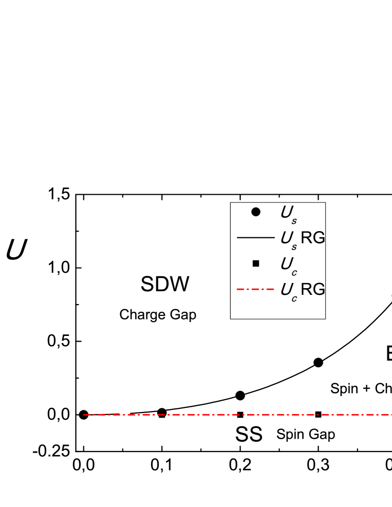
Figure 2: Solid circles (squares): critical value of the spin (charge) transition $U_{s}$ ($U_{c}$) as a function of $X$ obtained from the method of level crossings. Full line: solution of the RG equations given by Eq. (52). The dash dotted line at $U_{c}=0$ signal the boundary between the gapped and gapless charge phase as given by Eq. (46). The unit of energy is taken as $t=1$.

To compare the critical value of $U$ for the spin transition, we take $\lambda=4$, which using Eq. (53) and recalling that $v_{F}=a(t-X)$, leads to the same result as that obtained from vertex corrections Eq. (5) for small $X$. This leads to $A=\{4X/[\pi(t-X)]\}^{2}$. Replacing this result in Eq. (52), we obtain the function $U_{s}(X)$ that is represented in Fig. 2. The agreement with the numerical result up to $X/t\sim 0.4$ is excellent.

4 Summary and discussion

We have studied a field theory for the Hubbard model with small bond-charge interaction $X$ at half filling. While usually, it is enough to consider in the action only terms linear in the lattice parameter $a$, in our case it is necessary to include terms of order $a^{2}$ to obtain meaningful results at half filling. These terms can be classified in a similar way as the linear ones in terms of different processes in a ”$g$-ology” treatment (forward one branch, forward two branch, backward and Umklapp) but contain derivatives of the fields in the space direction.

We have obtained the RG equations of the different couplings using Operator Product Expansions. While the treatment of the new terms is awkward, most of them should be retained to keep the spin SU(2) invariance of the model.

According to the dominant correlations at large distances, the phases of the model can be classified as a singlet superconducting (SS) one for $U<U_{c}$, a bond ordering wave (BOW) for $U_{c}<U<U_{s}$ and a spin density wave (SDW) for $U>U_{s}$. The boundaries between the phases correspond to a charge transition for on site repulsion $U=U_{c}$ and a spin transition at $U=U_{s}$, which correspond respectively to the opening of a charge gap and a closing of the spin gap as $U$ increases. For the former transition we obtain $U_{c}=0$ in agreement with previous numerical studies for $X<0.5$ [35]. With only one adjustable parameter, we also obtain a very good agreement with the numerical results for $U_{s}$ if $X\lesssim 0.4t.$

To explain accurately the dependence of $U_{c}$ for $X>0.5$, it is necessary to go beyond our approach, possibly including more irrelevant operators.

As stated in Section 1.1, the model is an effective one-band model for a variety of physical systems, in particular optical lattices [12, 13, 14, 15]. In these systems, $U$ can be varied over the whole range, including its sign, through tuning of the external magnetic field $B$. It is also possible to change $X/t$ by 20%. Therefore, adjusting the filling to one particle per site, it seems in principle possible to tune the parameters in such a way the ground state of the system is in any of the three phases: SS, BOW or SDW.

Appendix A SU(2) spin rotational symmetry

In this appendix, we derive the relations among the constants $g^{\prime}$ which leave the theory invariant under spin SU(2) transformations.

Under an SU(2) rotation each spinor $\psi_{p\sigma}$, ($p=+,-$) transform as $\psi_{\sigma^{\prime}}^{\prime}=U_{\sigma^{\prime}\sigma}\psi_{\sigma}$ (the sum over repeated indices is implicitly understood). $\mathbf{U}$ is an SU(2) matrix given by:

$$\mathbf{U}=\left(\begin{array}[]{cc}a&b\\ -b^{\ast}&a^{\ast}\end{array}\right)$$ (55)

$a$ and $b$ are complex number satisfying $\mid a\mid^{2}+\mid b\mid^{2}=1$. We require the invariance of the $g$-ology Hamiltonian (12) under this rotation. We start by undertaking a rotation of the sum of the first terms of the second and the third line of (12). The transformed expression is:

$$- U_{\sigma_{1}\sigma}^{\ast}U_{\sigma\sigma_{2}}U_{\sigma_{3}\overline{\sigma}}^{\ast}U_{\overline{\sigma}\sigma_{4}}(\partial_{x}\psi_{\sigma_{1}+}^{\dagger}\psi_{\sigma_{2}+}\psi_{{\sigma_{3}}-}^{\dagger}\psi_{{\sigma_{4}}-}+\partial_{x}\psi_{\sigma_{1}+}^{\dagger}\psi_{\sigma_{2}-}\psi_{{\sigma_{3}}-}^{\dagger}\psi_{{\sigma_{4}}+})=$$ (56)

$$- U_{\sigma_{1}\sigma}^{\ast}U_{\sigma\sigma_{2}}U_{\sigma_{3}\overline{\sigma}}^{\ast}U_{\overline{\sigma}\sigma_{4}}\left(\partial_{x}\psi_{\sigma_{1}+}^{\dagger}\psi_{\sigma_{2}+}\psi_{{\sigma_{3}}-}^{\dagger}\psi_{{\sigma_{4}}-}-\partial_{x}\psi_{\sigma_{1}+}^{\dagger}\psi_{\sigma_{4}+}\psi_{\sigma_{3}-}^{\dagger}\psi_{\sigma_{2}-}+\delta_{\sigma_{2}\sigma_{3}}\psi_{\sigma_{1}+}^{\dagger}\psi_{\sigma_{4}+}\right)=$$

$$- \left(U_{\sigma_{1}\sigma}^{\ast}U_{\sigma\sigma_{2}}U_{\sigma_{3}\overline{\sigma}}^{\ast}U_{\overline{\sigma}\sigma_{4}}-U_{\sigma_{1}\sigma}^{\ast}U_{\sigma\sigma_{4}}U_{\sigma_{3}\overline{\sigma}}^{\ast}U_{\overline{\sigma}\sigma_{2}}\right)\partial_{x}\psi_{\sigma_{1}+}^{\dagger}\psi_{\sigma_{2}+}\psi_{{\sigma_{3}}-}^{\dagger}\psi_{{\sigma_{4}}-}$$

$$+ U_{\sigma_{1}\sigma}^{\ast}\underbrace{U_{\sigma\sigma_{2}}U_{\sigma_{2}\overline{\sigma}}^{\ast}}_{=\delta_{\sigma\overline{\sigma}}=0}U_{\overline{\sigma}\sigma_{4}}\psi_{\sigma_{1}+}^{\dagger}\psi_{\sigma_{4}+}$$

In the second term of the last line we have interchanged the dummy indices $\sigma_{2}$ with $\sigma_{4}$. Now it is possible to evaluate the difference of the products of U matrices involved in (56). We have:

$$U_{\sigma_{1}\sigma}^{\ast}U_{\sigma\sigma_{2}}U_{\sigma_{3}\overline{\sigma}}^{\ast}U_{\overline{\sigma}\sigma_{4}}-U_{\sigma_{1}\sigma}^{\ast}U_{\sigma\sigma_{4}}U_{\sigma_{3}\overline{\sigma}}^{\ast}U_{\overline{\sigma}\sigma_{2}} = U_{\sigma_{1}\sigma}^{\ast}U_{\sigma_{3}\overline{\sigma}}^{\ast}(\delta_{\sigma_{2}\overline{\sigma}_{4}}(\delta_{\sigma\sigma_{2}}-\delta_{\overline{\sigma}\sigma_{2}}))=$$

$$\delta_{\sigma_{2}\overline{\sigma}_{4}}(U_{\sigma_{1}\sigma_{2}}^{\ast}U_{\sigma_{3}\overline{\sigma}_{2}}^{\ast}-U_{\sigma_{1}\overline{\sigma}_{2}}^{\ast}U_{\sigma_{3}{\sigma_{2}}}^{\ast}) = \delta_{\sigma_{2}\overline{\sigma}_{4}}\delta_{\sigma_{3}\overline{\sigma}_{1}}(\delta_{\sigma_{1}\sigma_{2}}-\delta_{\sigma_{2}\sigma_{3}})$$ (57)

Inserting in (56) we obtain:

$$(\ref{g2g1rot}) = -(\partial_{x}\psi_{\sigma+}^{\dagger}\psi_{\sigma_{+}}\psi_{\overline{\sigma}-}^{\dagger}\psi_{\overline{\sigma}-}-\partial_{x}\psi_{\sigma+}^{\dagger}\psi_{\overline{\sigma}_{+}}\psi_{\overline{\sigma}-}^{\dagger}\psi_{{\sigma}-})=$$ (58)

$$-(\partial_{x}\psi_{\sigma+}^{\dagger}\psi_{\sigma_{+}}\psi_{\overline{\sigma}-}^{\dagger}\psi_{\overline{\sigma}-}+\partial_{x}\psi_{\sigma+}^{\dagger}\psi_{\sigma-}\psi_{\overline{\sigma}-}^{\dagger}\psi_{\overline{\sigma}+})$$

This is the sum of the first terms with the coefficients $g_{1\perp}^{\prime}$ and $g_{2\perp}^{\prime}$. Therefore we have shown that the sum of these terms is invariant under an SU(2) rotation. With the same procedure we can show indeed that the sum of all the terms multiplying $g_{1\perp}^{\prime}$ and the ones multiplying $g_{2\perp}^{\prime}$ transform into themselves by an SU(2) rotation. This implies that under the condition $g_{1\perp}^{\prime}=g_{2\perp}^{\prime}$, the Hamiltonian $H_{X}$ of Eq. (12) remains invariant.

Appendix B OPE’s between $O^{\prime}$ operators

In this appendix we give the expressions for all non-vanishing OPE’s between any two $O^{\prime}$ operators. The first one is:

$${O_{2.7}^{\prime}(z,\overline{z})}.{O_{1}^{\prime}(z^{\prime},\overline{z^{\prime}})}=\frac{1}{4\sqrt{2}\pi}\colon\partial_{z}\phi_{c-}(z)(\partial_{\overline{z}}\phi_{s+}(\overline{z}))^{2}\colon$$ (59)

$$\times \frac{2\pi\sqrt{2}}{L^{2}}\colon\cos(2\sqrt{2}\phi_{s}(z^{\prime},\overline{z}^{\prime})(\partial_{z^{\prime}}\phi_{c-}(z^{\prime})-\partial_{\overline{z}^{\prime}}\phi_{c+}(\overline{z}^{\prime}))\colon=$$

$$\frac{1}{2L^{2}}\bigg{(}\colon\cos(2\sqrt{2}\phi_{s}(z^{\prime},\overline{z}^{\prime}))(\partial_{\overline{z}^{\prime}}\phi_{s+})^{2}\colon+\frac{2\sqrt{2}}{\overline{z}^{\prime}-\overline{z}}\colon\sin(2\sqrt{2}\phi_{s+}(z^{\prime},\overline{z}^{\prime}))\partial_{\overline{z}}\phi_{s+}\colon$$

$$+\frac{2}{(\overline{z}^{\prime}-\overline{z})^{2}}\colon\cos(2\sqrt{2}\phi_{s}(z^{\prime},\overline{z}^{\prime}))\colon\bigg{)}\bigg{(}-\frac{1}{({z}^{\prime}-{z})^{2}}+\colon\partial_{z}\phi_{c-}\partial_{z^{\prime}}\phi_{c-}\colon-\partial_{z}\phi_{c-}\partial_{\overline{z}^{\prime}}\phi_{c+}\bigg{)}\simeq$$

$$\bigg{(}\frac{1}{L^{2}}\bigg{)}\frac{\colon\cos(2\sqrt{2}\phi_{s}(z,\overline{z}))\colon}{\mid{z}^{\prime}-{z}\mid^{4}}+...=\frac{1}{2\pi}\frac{O_{1}}{\mid{z}^{\prime}-{z}\mid^{4}}+...$$

To obtain the previous result we have first normal ordered each product of operators containing fields at different points. Then we have expanded the resulting expressions for $z^{\prime}$ near $z$. Let us show how we have proceeded step by step :

$$\partial_{z}\phi_{c-}(z)\;\;\partial_{z}\phi_{c-}(z^{\prime}) = (\partial_{z}\varphi_{c-}^{\dagger}(z)+\partial_{z}\varphi_{c-}(z))(\partial_{z^{\prime}}\varphi_{c-}^{\dagger}(z^{\prime})+\partial_{z^{\prime}}\varphi_{c-}(z^{\prime}))=$$ (60)

$$\partial_{z}\varphi_{c-}(z)\partial_{z^{\prime}}\varphi_{c-}({z^{\prime}})+\partial_{z}\varphi_{c-}^{\dagger}(z)\partial_{z^{\prime}}\varphi_{c-}^{\dagger}({z^{\prime}})+\partial_{z}\varphi_{c-}^{\dagger}(z)\partial_{z^{\prime}}\varphi_{c-}({z^{\prime}})+$$

$$\partial_{z^{\prime}}\varphi_{c-}^{\dagger}({z^{\prime}})\partial_{z}\varphi_{c-}(z)+\partial_{z}\partial_{z^{\prime}}[\varphi_{c-}(z),\varphi_{c-}^{\dagger}({z^{\prime}})]$$

and:

$$[\varphi_{c-}(z),\varphi_{c-}^{\dagger}({z^{\prime}})] =$$

$$\sum_{n_{p},n_{p^{\prime}}}\frac{e^{-pz}e^{p^{\prime}z^{\prime}}}{\sqrt{n_{p}n_{p}^{\prime}}}\underbrace{[b_{c-}^{p},b_{c-}^{p^{\prime}\dagger}]}_{\delta_{p,p^{\prime}}} = \sum_{n_{p}}\frac{e^{\frac{2\pi}{L}n_{p}(z^{\prime}-z)}}{n_{p}}\underbrace{=}_{\mid\underbrace{e^{\frac{2\pi}{L}(z^{\prime}-z)}\mid<1}_{\tau^{\prime}<\tau}}-\log(1-e^{\frac{2\pi}{L}(z-z^{\prime})})$$

$$\underbrace{\simeq}_{L>>\mid z^{\prime}-z\mid}-\log(\frac{2\pi}{L}(z-z^{\prime}))$$

$$\partial_{z}\partial_{z^{\prime}}[\varphi_{c-}(z),\varphi_{c-}^{\dagger}({z^{\prime}})] = -\frac{1}{(z-z^{\prime})^{2}}$$ (61)

The third equality has been taken from Ref. [62]. The condition $\tau^{\prime}<\tau$ implies that the operator should be time ordered in decreasing order from left to right. Including Eq. (61) in Eq. (60) we obtain:

$$\partial_{z}\phi_{c-}(z)\;\;\partial_{z}\phi_{c-}(z^{\prime})=\colon\partial_{z}\phi_{c-}(z)\;\;\partial_{z}\phi_{c-}(z^{\prime})\colon-\frac{1}{(z-z^{\prime})^{2}}$$ (62)

which is the result used in Eq. (59). Regarding the normal ordering of the product $\colon(\partial_{\overline{z}}\phi_{s+}(\overline{z}))^{2}\colon\;\;\colon\cos(2\sqrt{2}\phi_{s}(z^{\prime},\overline{z}^{\prime})\colon$, we use the following basic OPE:

$$\partial_{\overline{z}}\varphi_{s+}(\overline{z})e^{i\lambda\varphi_{s}^{\dagger}(\overline{z}^{\prime})}=$$

$$e^{i\lambda\varphi_{s}^{\dagger}(\overline{z}^{\prime})}\partial_{\overline{z}}\varphi_{s+}(\overline{z})+i{\lambda}\underbrace{[\partial_{\overline{z}}\varphi_{s+}(\overline{z}),\underbrace{\varphi_{s}^{\dagger}(\overline{z}^{\prime})}_{\frac{(\varphi_{s+}^{\dagger}+\varphi_{s-}^{\dagger})}{2}}]}_{\frac{1}{2(\overline{z}^{\prime}-\overline{z})}}e^{i\lambda\varphi_{s}^{\dagger}(\overline{z}^{\prime})}$$ (63)

where we have used $Ae^{B}=e^{B}A+[A,B]e^{B}$ and the commutator was calculated as in Eq. (61). Therefore, we have:

$$\partial_{\overline{z}}\varphi_{s+}(\overline{z})\colon\cos(2\sqrt{2}\phi_{s}(z^{\prime},\overline{z}^{\prime}))\colon=$$

$$\colon\cos(2\sqrt{2}\phi_{s}(z^{\prime},\overline{z}^{\prime}))\partial_{\overline{z}}\varphi_{s+}(\overline{z}):-\frac{\sqrt{2}}{(\overline{z}^{\prime}-\overline{z})}\colon\sin(2\sqrt{2}\phi_{s}(z^{\prime},\overline{z}^{\prime}))\colon$$ (64)

(the last sign changes if one permutes sin and cos) and:

$$(\partial_{\overline{z}}\varphi_{s+}(\overline{z}))^{2}\colon\cos(2\sqrt{2}\phi_{s}(z^{\prime},\overline{z}^{\prime}))\colon=$$

$$\partial_{\overline{z}}\varphi_{s+}(\overline{z})\bigg{(}\colon\cos(2\sqrt{2}\phi_{s}(z^{\prime},\overline{z}^{\prime}))\colon\partial_{\overline{z}}\varphi_{s+}(\overline{z})-\frac{\sqrt{2}}{(\overline{z}^{\prime}-\overline{z})}\colon\sin(2\sqrt{2}\phi_{s}(z^{\prime},\overline{z}^{\prime}))\colon\bigg{)}=$$

$$\bigg{(}\colon\cos(2\sqrt{2}\phi_{s}(z^{\prime},\overline{z}^{\prime}))\colon\partial_{\overline{z}}\varphi_{s+}(\overline{z})-\frac{\sqrt{2}}{(\overline{z}^{\prime}-\overline{z})}\colon\sin(2\sqrt{2}\phi_{s}(z^{\prime},\overline{z}^{\prime}))\colon\bigg{)}\partial_{\overline{z}}\varphi_{s+}(\overline{z})$$

$$-\frac{\sqrt{2}}{(\overline{z}^{\prime}-\overline{z})}\bigg{(}\colon\sin(2\sqrt{2}\phi_{s}(z^{\prime},\overline{z}^{\prime}))\colon\partial_{\overline{z}}\varphi_{s+}+$$

$$\frac{\sqrt{2}}{(\overline{z}^{\prime}-\overline{z})}\colon\cos(2\sqrt{2}\phi_{s}(z^{\prime},\overline{z}^{\prime}))\colon\bigg{)}=$$

$$\colon\cos(2\sqrt{2}\phi_{s}(z^{\prime},\overline{z}^{\prime}))\colon\bigg{(}(\partial_{\overline{z}}\varphi_{s+}(\overline{z}))^{2}-\frac{2}{(\overline{z}^{\prime}-\overline{z})^{2}}\bigg{)}$$

$$-\frac{2\sqrt{2}}{(\overline{z}^{\prime}-\overline{z})}\colon\sin(2\sqrt{2}\phi_{s}(z^{\prime},\overline{z}^{\prime}))\colon\partial_{\overline{z}}\varphi_{s+}(\overline{z})$$ (65)

The required OPE is:

$$\colon(\partial_{\overline{z}}\phi_{s+}(\overline{z}))^{2}\colon\;\;\colon\cos(2\sqrt{2}\phi_{s}(z^{\prime},\overline{z}^{\prime})\colon=$$

$$\bigg{[}(\partial_{\overline{z}}\varphi_{s+}(\overline{z}))^{2}+2(\partial_{\overline{z}}\varphi_{s+}^{\dagger}(\overline{z}))(\partial_{\overline{z}}\varphi_{s+}(\overline{z}))+(\partial_{\overline{z}}\varphi_{s+}^{\dagger})^{2}\bigg{]}\colon\cos(2\sqrt{2}\phi_{s}(z^{\prime},\overline{z}^{\prime})\colon=$$

$$\colon\cos(2\sqrt{2}\phi_{s}(z^{\prime},\overline{z}^{\prime}))(\partial_{\overline{z}^{\prime}}\phi_{s+})^{2}\colon$$

$$-\frac{2\sqrt{2}}{\overline{z}^{\prime}-\overline{z}}\colon\sin(2\sqrt{2}\phi_{s+}(z^{\prime},\overline{z}^{\prime}))\colon-\frac{2}{(\overline{z}^{\prime}-\overline{z})^{2}}\colon\cos(2\sqrt{2}\phi_{s}(z^{\prime},\overline{z}^{\prime})\colon$$ (66)

which is the other OPE used in Eq. (59).

An analogous reasoning leads to the remaining non-vanishing OPE’s:

$${O_{2.3}^{\prime}(z,\overline{z})}{O_{1}^{\prime}(z^{\prime},\overline{z^{\prime}})}=-\frac{1}{4\sqrt{2}\pi}\colon\partial_{\overline{z}}\phi_{c+}({\overline{z}})(\partial_{z}\phi_{s-}(z))^{2}\colon$$

$$\times\frac{2\pi\sqrt{2}}{L^{2}}\colon\cos(2\sqrt{2}\phi_{s}(z^{\prime},\overline{z}^{\prime})(\partial_{z^{\prime}}\phi_{c-}(z^{\prime})-\partial_{\overline{z}^{\prime}}\phi_{c+}(\overline{z}))\colon=$$

$$-\frac{1}{2L^{2}}\bigg{(}\colon\cos(2\sqrt{2}\phi_{s}(z^{\prime},\overline{z}^{\prime}))(\partial_{z^{\prime}}\phi_{s-})^{2}\colon+\frac{2\sqrt{2}}{z^{\prime}-z}\colon\sin(2\sqrt{2}\phi_{s+}(z^{\prime},\overline{z}^{\prime}))\partial_{z}\phi_{s-}\colon$$

$$+\frac{2}{(z^{\prime}-z)^{2}}\colon\cos(2\sqrt{2}\phi_{s}(z^{\prime},\overline{z}^{\prime}))\colon\bigg{)}\bigg{(}+\frac{1}{(\overline{z}-\overline{z}^{\prime})^{2}}+\partial_{\overline{z}}\phi_{c+}\partial_{\overline{z}^{\prime}}\phi_{c-}-\colon\partial_{\overline{z}}\phi_{c+}\partial_{\overline{z}^{\prime}}\phi_{c+}\colon\bigg{)}\simeq$$

$$\bigg{(}\frac{1}{L^{2}}\bigg{)}\frac{\colon\cos(2\sqrt{2}\phi_{s}(z,\overline{z})}{\mid{z}^{\prime}-{z}\mid^{4}\colon}+...=\frac{1}{2\pi}\frac{O_{1}}{\mid{z}^{\prime}-{z}\mid^{4}}+...$$ (67)

$${O_{2.2}^{\prime}(z,\overline{z})}{O_{3}^{\prime}(z^{\prime},\overline{z}^{\prime})}=\frac{1}{4\sqrt{2}\pi}\colon\partial_{\overline{z}}\phi_{c+}({\overline{z}})(\partial_{z}\phi_{c-}(z))^{2}\colon$$

$$\times\frac{2\pi\sqrt{2}}{L^{2}}\colon\cos(2\sqrt{2}\phi_{c}(z^{\prime},\overline{z}^{\prime}))(\partial_{z^{\prime}}\phi_{c-}(z^{\prime})-\partial_{\overline{z}^{\prime}}\phi_{c+}(\overline{z}^{\prime}))\colon\simeq$$

$$-\bigg{(}\frac{1}{L^{2}}\bigg{)}\frac{\colon\cos(2\sqrt{2}\phi_{c}(z,\overline{z}))\colon}{\mid{z}^{\prime}-{z}\mid^{4}}+...=-\frac{1}{2\pi}\frac{O_{3}}{\mid{z}^{\prime}-{z}\mid^{4}}+...$$ (68)

$${O_{2.5}^{\prime}(z,\overline{z})}{O_{3}^{\prime}(z^{\prime},\overline{z}^{\prime})}=-\frac{1}{4\sqrt{2}\pi}\colon\partial_{{z}}\phi_{c-}({z})(\partial_{{\overline{z}}}\phi_{c+}({\overline{z}}))^{2}\colon$$

$$\times\frac{2\pi\sqrt{2}}{L^{2}}\colon\cos(2\sqrt{2}\phi_{c}(z^{\prime},\overline{z}^{\prime}))(\partial_{z^{\prime}}\phi_{c-}(z^{\prime})-\partial_{\overline{z}^{\prime}}\phi_{c+}(\overline{z}^{\prime}))\colon=$$

$$-\bigg{(}\frac{1}{2L^{2}}\bigg{)}\partial_{z}\phi_{c-}\bigg{(}\colon\cos(2\sqrt{2}\phi_{c}(z^{\prime},\overline{z}^{\prime}))(\partial_{\overline{z}}\phi_{c+})^{2}\partial_{{z}}\phi_{c-}\colon-\frac{2\sqrt{2}}{\overline{z^{\prime}}-\overline{z}}\colon\sin(2\sqrt{2}\phi_{c}(z^{\prime},\overline{z}^{\prime}))\partial_{\overline{z}}\phi_{c+}\partial_{z^{\prime}}\phi_{c-}\colon$$

$$-\frac{2}{(\overline{z^{\prime}}-\overline{z})^{2}}\colon\cos(2\sqrt{2}\phi_{c}(z^{\prime},\overline{z}^{\prime}))\partial_{z^{\prime}}\phi_{c-}\colon\bigg{)}\simeq$$

$$-\bigg{(}\frac{1}{L^{2}}\bigg{)}\frac{\colon\cos(2\sqrt{2}\phi_{c}(z,\overline{z}))\colon}{\mid{z}^{\prime}-{z}\mid^{4}}+...=-\frac{1}{2\pi}\frac{O_{3}}{\mid{z}^{\prime}-{z}\mid^{4}}+...$$ (69)

$${O_{2.3}^{\prime}(z,\overline{z})}{O_{2.4}^{\prime}(z^{\prime},\overline{z}^{\prime})}=-\frac{1}{8}\bigg{(}\frac{1}{\sqrt{2}\pi}\colon\partial_{\overline{z}}\phi_{c+}(\overline{z})(\partial_{z}\phi_{s-}(z))^{2}\colon\bigg{)}$$

$$\times\bigg{(}\frac{1}{\sqrt{2}\pi}\colon\partial_{\overline{z}^{\prime}}\phi_{c+}(\overline{z}^{\prime})\partial_{z^{\prime}}\phi_{s-}(z^{\prime})\partial_{\overline{z}^{\prime}}\phi_{s+}(\overline{z^{\prime}})\colon\bigg{)}=$$

$$-\frac{1}{16\pi^{2}}\bigg{(}\colon(\partial_{z}\phi_{s-}(z))^{2}\partial_{z^{\prime}}\phi_{s-}(z^{\prime})\colon-\frac{2\partial_{z}\phi_{s-}(z)}{(z-z^{\prime})^{2}}\bigg{)}$$

$$\times\bigg{(}\colon\partial_{\overline{z}}\phi_{c+}(\overline{z})\;\;\partial_{\overline{z^{\prime}}}\phi_{c+}(\overline{z^{\prime}})\colon-\frac{1}{(\overline{z}-\overline{z}^{\prime})^{2}}\bigg{)}\partial_{\overline{z}^{\prime}}\phi_{s+}(\overline{z}^{\prime})\simeq$$

$$-\frac{1}{8\pi^{2}}\frac{\partial_{\overline{z}}\phi_{s+}(\overline{z})\partial_{z}\phi_{s-}(z)}{\mid z-z^{\prime}\mid^{4}}+...=\frac{1}{2\pi}\frac{O_{2s}}{\mid{z}^{\prime}-{z}\mid^{4}}+...$$ (70)

$${O_{2.7}^{\prime}(z,\overline{z})}{O_{2.6}^{\prime}(z^{\prime},\overline{z}^{\prime})}=-\frac{1}{8}\bigg{(}\frac{1}{\sqrt{2}\pi}\colon\partial_{z}\phi_{c-}(z)(\partial_{\overline{z}}\phi_{s+}(\overline{z}))^{2}\colon\bigg{)}$$

$$\times\bigg{(}\frac{1}{\sqrt{2}\pi}\colon\partial_{z^{\prime}}\phi_{c-}(z^{\prime})\partial_{z^{\prime}}\phi_{s-}(z^{\prime})\partial_{\overline{z}^{\prime}}\phi_{s+}(\overline{z^{\prime}})\colon\bigg{)}=$$

$$-\frac{1}{16\pi^{2}}\bigg{(}\colon(\partial_{\overline{z}}\phi_{s+}(\overline{z}))^{2}\partial_{\overline{z}^{\prime}}\phi_{s+}(\overline{z}^{\prime})\colon-\frac{2\partial_{\overline{z}}\phi_{s+}(\overline{z})}{(\overline{z}-\overline{z}^{\prime})^{2}}\bigg{)}$$

$$\times\bigg{(}\colon\partial_{{z}}\phi_{c-}({z})\;\;\partial_{{z^{\prime}}}\phi_{c-}({z^{\prime}})\colon-\frac{1}{(z-z^{\prime})^{2}}\bigg{)}\partial_{{z}^{\prime}}\phi_{s-}({z}^{\prime})=$$

$$-\frac{1}{8\pi^{2}}\frac{\partial_{\overline{z}}\phi_{s+}(\overline{z})\partial_{z}\phi_{s-}(z)}{\mid z-z^{\prime}\mid^{4}}+...=\frac{1}{2\pi}\frac{O_{2s}}{\mid{z}^{\prime}-{z}\mid^{4}}+...$$ (71)

$${O_{2.4}^{\prime}(z,\overline{z})}{O_{2.6}^{\prime}(z^{\prime},\overline{z}^{\prime})}=\frac{1}{16}\bigg{(}\frac{2}{\sqrt{2}\pi}\colon\partial_{\overline{z}}\phi_{c+}(\overline{z})\partial_{z}\phi_{s-}(z)\partial_{\overline{z}}\phi_{s+}(\overline{z})\colon\bigg{)}$$

$$\times\bigg{(}\frac{2}{\sqrt{2}\pi}\colon\partial_{z^{\prime}}\phi_{c-}(z^{\prime})\partial_{z^{\prime}}\phi_{s-}(z^{\prime})\partial_{\overline{z}^{\prime}}\phi_{s+}(\overline{z^{\prime}})\colon\bigg{)}\simeq$$

$$\frac{1}{8\pi^{2}}\frac{\partial_{\overline{z}}\phi_{c+}(\overline{z})\partial_{z}\phi_{c-}(z)}{\mid z-z^{\prime}\mid^{4}}+...=\frac{1}{2\pi}\frac{O_{2c}}{\mid{z}^{\prime}-{z}\mid^{4}}+...$$ (72)

$${O_{2.2}^{\prime}(z,\overline{z})}{O_{2.5}^{\prime}(z^{\prime},\overline{z}^{\prime})}=\frac{1}{32\pi^{2}}\bigg{(}\colon(\partial_{z}\phi_{c-}(z))^{2}\partial_{\overline{z}}\phi_{c+}(\overline{z})\colon\bigg{)}\;\;\bigg{(}\colon\partial_{z^{\prime}}\phi_{c-}(z^{\prime})(\partial_{\overline{z}^{\prime}}\phi_{c+}(\overline{z}^{\prime}))^{2}\colon\bigg{)}=$$

$$\frac{1}{32\pi^{2}}\bigg{(}\colon(\partial_{z}\phi_{c-}(z))^{2}\partial_{z^{\prime}}\phi_{c-}({z}^{\prime})\colon-\frac{2\partial_{z}\phi_{c-}}{({z}^{\prime}-{z})^{2}}\bigg{)}\bigg{(}\colon\partial_{\overline{z}}\phi_{c+}(\overline{z})(\partial_{z^{\prime}}\phi_{c+}(\overline{z}^{\prime}))^{2}\colon-\frac{2\partial_{\overline{z}}\phi_{c+}}{(\overline{z}^{\prime}-\overline{z})^{2}}\bigg{)}\simeq$$

$$\frac{1}{8\pi^{2}}\frac{\partial_{\overline{z}}\phi_{c+}(\overline{z})\partial_{z}\phi_{c-}(z)}{\mid z-z^{\prime}\mid^{4}}+...=\frac{1}{2\pi}\frac{O_{2c}}{\mid{z}^{\prime}-{z}\mid^{4}}+...$$ (73)

References

- [1] M. E. Foglio and L. M. Falicov, Phys. Rev. B 20 (1979) 4554.
- [2] S. Kivelson, W.-P. Su, J. R. Schrieffer, and A. J. Heeger, Phys. Rev. Lett. 58 (1987) 1899.
- [3] D. Baeriswyl, Peter Horsch, and K. Maki, Phys. Rev. Lett. 60 (1988) 70.
- [4] J. T. Gammel and D. K. Campbell, Phys. Rev. Lett. 60 (1988) 71.
- [5] Y. Z. Zhang, Phys. Rev. B 92 (2004) 246404.
- [6] R. Strack and D. Volhardt, Phys. Rev. Lett. 70 (1993) 2637.
- [7] A. A. Aligia, L. Arrachea and E. R. Gagliano, Phys. Rev. B 51 (1995) 13774.
- [8] F. Marsiglio and J. E. Hirsch, Phys. Rev. B 49 (1994) 1366.
- [9] H. B. Schüttler and A. J. Fedro, Phys. Rev. B 45 (1992) 7588.
- [10] M. E. Simon and A. A. Aligia, Phys. Rev. B 48, (1993) 7471.
- [11] M. E. Simon, A. A. Aligia and E. R. Gagliano, Phys. Rev. B 56 (1997) 5637.
- [12] L. M. Duan, Europhys. Lett. 81 (2008) 20001.
- [13] T. Goodman and L. M. Duan, Phys. Rev. A 79 (2009) 023617.
- [14] J. P. Kestner and L.-M. Duan, Phys. Rev. A 81 (2010) 043618.
- [15] L. M. Duan, Phys. Rev. Lett. 95 (2005) 243202.
- [16] A. Hübsch, J. C. Lin, J. Pan, and D. L. Cox, Phys. Rev. Lett. 96 (2006) 196401.
- [17] S. Raghu, S. A. Kivelson, and D. J. Scalapino, Phys. Rev. B 81 (2010) 224505.
- [18] L. Arrachea and A. A. Aligia, Phys. Rev. B 61 (2000) 9686.
- [19] L. Arrachea and A. A. Aligia, Phys. Rev. B 59 (1999) 1333.
- [20] G. I. Japaridze and A. P. Kampf, Phys. Rev. B 59 (1999) 12822.
- [21] A. A. Aligia and L. Arrachea, Phys. Rev. B 60 (1999) 15332.
- [22] A. A. Aligia, K. Hallberg, C.D. Batista and G. Ortiz, Phys. Rev. B 61 (2000) 7883.
- [23] I. N. Karnaukhov, Phys. Rev. Lett. 74 (1995) 5285.
- [24] J. E. Hirsch, Physica C 158 (1989) 326.
- [25] J. E. Hirsch and F. Marsiglio, Phys. Rev. B 39 (1989) 11515.
- [26] G. I. Japaridze and E. Müller-Hartman, Ann. Phys. 3 (1994) 163.
- [27] L. Arrachea, A. A. Aligia, E. Gagliano, K. Hallberg, and C. Balseiro, Phys. Rev. B 50 (1994) 16044.
- [28] B. R. Bulka, Phys. Rev. B 57 (1998) 10303.
- [29] L. Arrachea and A. A. Aligia, Phys. Rev. Lett. 73 (1994) 2240.
- [30] J. de Boer, V. E. Korepin, and A. Schadschneider, Phys. Rev. Lett. 74 (1995) 789.
- [31] L. Arrachea, A. A. Aligia and E. Gagliano, Phys. Rev. Lett. 76 (1996) 4396.
- [32] A. Anfossi, P. Giorda, A. Montorsi, and F. Traversa, Phys. Rev. Lett. 95 (2005) 056402.
- [33] A. Anfossi, P. Giorda, and A. Montorsi, Phys. Rev. B 75 (2007) 165106.
- [34] A. Anfossi, C. Degli Esposti Boschi, A. Montorsi, and F. Ortolani, Phys. Rev. B 73 (2006) 085113.
- [35] A. A. Aligia, A. Anfossi, L. Arrachea, C. Degli Esposti Boschi, A. O. Dobry, C. Gazza, A. Montorsi, F. Ortolani, and M. E. Torio, Phys. Rev. Lett. 99 (2007) 206401.
- [36] A. Anfossi, C. Degli Esposti Boschi, A. Montorsi Phys. Rev. B 79 (2009) 235117.
- [37] M. E. Torio, A. A. Aligia, G. I. Japaridze, and B. Normand, Phys. Rev. B 73 (2006) 115109.
- [38] M. Nakamura, Phys. Rev. B 61 (2000) 16377.
- [39] A. A. Aligia and G. Ortiz, Phys. Rev. Lett. 82 (1999) 2560.
- [40] R. Resta and S. Sorella, Phys. Rev. Lett. 82 (1999) 370.
- [41] G. Ortiz and A. A. Aligia, Physica Status Solidi (b) 220 (2000) 737.
- [42] C. D. Batista, G. Ortiz, and A. A. Aligia, Phys. Rev. Lett. 101 (2008) 077203.
- [43] M. Nakamura and S. Todo, Phys. Rev. Lett. 89 (2002) 077204.
- [44] G. I. Japaridze, R. M. Noack, D. Baeriswyl, , and L. Tincani, Phys. Rev. B 76 (2007) 115118.
- [45] A. A. Nersesyan, A. O. Gogolin, and F.H.L. Eler, Phys. Rev. Lett. 81 (1998) 910.
- [46] M. Fabrizio, A. O. Gogolin, and A. A. Nersesyan, Phys. Rev. Lett. 83 (1999) 2014.
- [47] M. Fabrizio, A. O. Gogolin, and A. A. Nersesyan, Nucl. Phys. B 580 (2000) 647.
- [48] M.E. Torio, A.A. Aligia, and H.A. Ceccatto, Phys. Rev. B 64 (2001) 121105(R).
- [49] S. R. Manmana, V. Meden, R. M. Noack, and K. Schönhammer, Phys. Rev. B 70 (2004) 155115.
- [50] A. A. Aligia, Phys. Rev. B 69, 041101(R) (2004)
- [51] C. D. Batista and A. A. Aligia, Phys. Rev. Lett. 92 (2004) 246405.
- [52] A. A. Aligia and C. D. Batista, Phys. Rev. B 71 (2005) 125110.
- [53] L. Tincani, R. M. Noack, and D. Baeriswyl, Phys. Rev. B 79 (2009) 165109.
- [54] A. Montorsi, private communication.
- [55] M. Roncaglia, C. Degli Esposti Boschi and A. Montorsi, preprint ”Effective theory for the Hirsch model in the incommensurate singlet superconducting phase”
- [56] M. Tsuchiizu and A. Furusaki, Phys. Rev. B 69 (2004) 035103.
- [57] arXiv:hep-th/9210046. Lectures presented at TASI 1992.
- [58] T. Giamarchi, Quantum Physics in One Dimension (Oxford University Press, Oxford, U.K., 2004).
- [59] Daniel J. Amit, Victor Martin Mayor, Field Theory; The Renormalization Group and Critical Phenomena. World Scienfic (2005)
- [60] J. von Delft and H. Schoeller, Annalen Phys. 7 (1998) 225-305.
- [61] J Cardy, Scaling and renormalization in statistical physics (Cambridge University Press, 1996.), chapter 5.
- [62] Complex Variables and Applications (Ruel V. Churchill and James Ward Brown, McGraw-Hill, 2008).