Low scale saturation of Effective NN Interactions and their Symmetries

Abstract

The Skyrme force parameters can be uniquely determined by coarse graining the NN interactions at a characteristic momentum scale. We show how exact $V_{\rm lowk}$ potentials to second order in momenta are accurately and universally saturated with physical NN scattering threshold parameters at CM momentum scales of about $\Lambda=250{\rm MeV}$ for the S-waves and $\Lambda=100{\rm MeV}$ for the P-waves. The pattern of Wigner and Serber symmetries unveiled previously is also saturated at these scales.

The derivation of effective interactions from NN dynamics has been a major task in Nuclear Physics ever since the pioneering works of Moshinsky Moshinsky (1958) and Skyrme Skyrme (1959). The use of those effective potentials, referred to as Skyrme forces, in mean field calculations can hardly be exaggerated due to the enormous simplifications that are implied as compared to the original many-body problem Vautherin and Brink (1972); Negele and Vautherin (1972); Chabanat et al. (1997); Bender et al. (2003). Similar ideas advanced by Moszkowski and Scott Moszkowski and Scott (1960) have become rather useful in Shell model calculations Dean et al. (2004); Coraggio et al. (2009). The Skyrme (pseudo)potential is usually written in coordinate space and contains delta functions and its derivatives Skyrme (1959). In momentum space it corresponds to a power expansion in the CM momenta $({\bf p^{\prime}}$ and ${\bf p})$ corresponding to the initial and final state respectively. To second order in momenta the potential reads

$$V({\bf p}^{\prime},{\bf p})=\int d^{3}xe^{-i{\bf x}\cdot({\bf p^{\prime}}-{\bf p})}V({\bf x})$$ (1)

$$= t_{0}(1+x_{0}P_{\sigma})+\frac{t_{1}}{2}(1+x_{1}P_{\sigma})({\bf p}^{\prime 2}+{\bf p}^{2})$$

$$+ t_{2}(1+x_{2}P_{\sigma}){\bf p}^{\prime}\cdot{\bf p}+2iW_{0}{\bf S}\cdot({\bf p}^{\prime}\wedge{\bf p})$$

$$+ \frac{t_{T}}{2}\left[\sigma_{1}\cdot{\bf p}\,\sigma_{2}\cdot{\bf p}+\sigma_{1}\cdot{\bf p^{\prime}}\,\sigma_{2}\cdot{\bf p^{\prime}}-\frac{1}{3}\sigma_{1}\,\cdot\sigma_{2}({\bf p^{\prime}}^{2}+{\bf p}^{2})\right]$$

$$+ \frac{t_{U}}{2}\left[\sigma_{1}\cdot{\bf p}\,\sigma_{2}\cdot{\bf p}^{\prime}+\sigma_{1}\cdot{\bf p^{\prime}}\,\sigma_{2}\cdot{\bf p}-\frac{2}{3}\sigma_{1}\,\cdot\sigma_{2}{\bf p^{\prime}}\cdot{\bf p}\right]$$

where $P_{\sigma}=(1+\sigma_{1}\cdot\sigma_{2})/2$ is the spin exchange operator with $P_{\sigma}=-1$ for spin singlet $S=0$ and $P_{\sigma}=1$ for spin triplet $S=1$ states. In practice, these effective forces are parameterized in terms of a few constants which encode the relevant physical information and should be deduced directly from the elementary and underlying NN interactions. Unfortunately, there is a huge variety of Skyrme forces depending on the fitting strategy employed (see e.g. Friedrich and Reinhard (1986); Klupfel et al. (2009)). This lack of uniqueness may indicate that the systematic and/or statistical uncertainties within the various schemes are not accounted for completely. Interestingly, the natural units for those parameters have been outlined in Ref. Furnstahl and Hackworth (1997); Kortelainen et al. (2010) yielding the correct order of magnitude. A microscopic basis Baldo et al. (2010); Stoitsov et al. (2010) for the Density Functional Theory (DFT) approach has also been set up, but still uncertainties remain.

Although the pseudo-potential in Eq. (1) may be taken literally in mean field calculations, due to the finite extension of the nucleus, its interpretation in the simplest two-body problem requires some regularization to give a precise meaning to the Dirac delta interactions. The standard view of a pseudo-potential (in the sense of Fermi) is that it corresponds to the potential which in the Born approximation yields the real part of the full scattering amplitude. This is a prescription which implements unitarity, but necessarily fails when the scattering length is unnaturally large as it is the case for NN interactions. On the contrary, the Wilsonian viewpoint corresponds to a coarse graining of the NN interaction to a certain energy scale. There are several schemes to coarse grain interactions in Nuclear Physics. The traditional way has been by using the oscillator shell model, where matrix elements of NN interactions are evaluated with oscillator constants of about $b=1.4-2\,{\rm fm}$ Coraggio et al. (2009). A modern way of coarse graining nuclear interactions is represented by the $V_{\rm lowk}$ method Bogner et al. (2003a) (for a review see Bogner et al. (2010)) where all momentum scales above $2{\rm fm}^{-1}$ are integrated out. The recent Euclidean Lattice Effective Field Theory (EFT) calculations (for a review see e.g. Lee (2009)), although breaking rotational symmetry explicitly, provide a competitive scheme where coarse grained interactions allow ab initio calculations combining the insight of EFT and Monte-Carlo lattice experience, with lattice spacings as large as $a=2{\rm fm}$. These length scales match the typical inter-particle distance of nuclear matter $d=1/\rho^{\frac{1}{3}}\sim 2{\rm fm}$. Actually, the three approaches feature energy-, momentum- and configuration space coarse graining respectively and ignore explicit dynamical effects below distances $\sim b\sim 1/\Lambda\sim a$ which advantageously sidestep the problems related to the hard core and confirm the modern view that ab initio calculations are subjected to larger systematic uncertainties than assumed hitherto. Clearly, any computational set up implementing the coarse graining philosophy yields by itself a unique definition of the effective interaction. However, there is no universal effective interaction definition. For definiteness, we will follow here the $V_{\rm lowk}$ scheme to determine the effective parameters because within this framework some underlying old nuclear symmetries, namely those implied by Wigner and Serber forces, are vividly displayed Calle Cordon and Ruiz Arriola (2008, 2009); Ruiz Arriola and Calle Cordon (2009); Arriola and Cordon (2010).

In the present paper we want to show that in fact these parameters can uniquely be determined from known NN scattering threshold parameters by rather simple calculations by just coarse grain the interaction over all wavelengths larger than the typical ones occurring in finite nuclei. As we will show, this introduces a momentum scale $\Lambda$ in the 9 effective parameters $t_{0,1,2}$, $x_{0,1,2}$ and $t_{U,T,V}$ which allow to connect the two body problem to the many body problem. Going beyond Eq. (1) requires further information than just two-body low energy scattering, in particular knowledge about three and four body forces and their scale dependence consistently inherited from their NN counterpart. The finite $k_{F}$ situation relevant for heavy nuclei and nuclear matter involves mixing between operators with different particle number and, in principle, could be conveniently tackled with the method outlined in Ref. de la Plata and Salcedo (1998) where the lack of genuine medium effects is manifestly built in.

For completeness, we review here the $V_{\rm lowk}$ approach Bogner et al. (2003b) in a way that our points can be easily stated. The starting point is a given phenomenological NN potential, $V$, and usually denominated bare potential, whence the scattering amplitude or $T$ matrix is obtained as the solution of the half-off shell Lippmann-Schwinger (LS) coupled channel equation in the CM system

$$T_{l^{\prime},l}^{J}(k^{\prime},k;k^{2})=V_{l^{\prime},l}^{J}(k^{\prime},k)$$

$$+\sum_{l^{\prime\prime}}\int_{0}^{\infty}\,\frac{M_{N}}{(2\pi)^{3}}\frac{dq\,q^{2}}{k^{2}-q^{2}}V_{l^{\prime},l^{\prime\prime}}^{J}(k^{\prime},q)T_{l^{\prime\prime},l}^{J}(q,k;k^{2})\,,$$ (2)

where $J$ is the total angular momentum and $l,l^{\prime}$ are orbital angular momentum quantum numbers $p,p^{\prime},q$ are CM momenta and $M_{N}$ is the Nucleon mass. The unitary (coupled channel) S-matrix is obtained as usual

$$S_{l^{\prime},l}^{J}(p)=\delta_{l^{\prime},l}-{\rm i}\frac{pM_{N}}{8\pi^{2}}T_{l^{\prime},l}^{J}(p,p)\,.$$ (3)

Using the matrix representation ${\bf S}^{J}=({\bf M}^{J}-i{\bf 1})({\bf M}^{J}+i{\bf 1})^{-1}$ with $({\bf M}^{J})^{\dagger}={\bf M}^{J}$ a hermitian coupled channel matrix, at low energies the effective range theory for coupled channels reads

$$p^{l+l^{\prime}+1}M_{l^{\prime},l}^{J}(p)=-(\alpha^{-1})^{J}_{l,l^{\prime}}+\frac{1}{2}(r)^{J}_{l,l^{\prime}}p^{2}+(v)^{J}_{l,l^{\prime}}p^{4}+\dots$$ (4)

which in the absence of mixing and using $S_{l}(p)=e^{2i\delta_{l}(p)}$ reduces to the well-known expression

$$p^{2l+1}\cot\delta_{l}(p)=-\frac{1}{\alpha_{l}}+\frac{1}{2}r_{l}p^{2}+v_{l}p^{4}+\dots$$ (5)

An extensive study and determination of the low energy parameters for all partial waves has been carried out in Ref. Pavon Valderrama and Arriola (2005) for both the NijmII and the Reid93 potentials Stoks et al. (1994) yielding similar numerical results. Dropping these coupled channel indices for simplicity the $V_{\rm lowk}$ potential is then defined by the equation

$$T(k^{\prime},k;k^{2})=V_{\rm lowk}(k^{\prime},k)$$

$$+\int_{0}^{\Lambda}\,\frac{M_{N}}{(2\pi)^{3}}\frac{dq\,q^{2}}{k^{2}-q^{2}}V_{\rm lowk}(k^{\prime},q)T(q,k;k^{2})\,,$$ (6)

where $(k,k^{\prime})\leq\Lambda$. We use here a sharp three-dimensional cut-off $\Lambda$ to separate between low and high momenta since our results are not sensitive to the specific form of the regularization. Thus, eliminating the $T$ matrix we get the equation for the effective potential which evidently depends on the cut-off scale $\Lambda$ and corresponds to the effective interaction which nucleons see when all momenta higher then the momentum scale $\Lambda$ are integrated out. It has been found Bogner et al. (2003b) that high precision potential models, i.e. fitting the NN data to high accuracy incorporating One Pion Exchange (OPE) at large distances and describing the deuteron form factors, collapse into a unique self-adjoint nonlocal potential for $\Lambda\sim 400-450{\rm MeV}$. This is a not a unreasonable result since all the potentials provide a rather satisfactory description of elastic NN scattering data up to $p\sim 400{\rm MeV}$. Note that this universality requires a marginal effect of off-shell ambiguities (beyond OPE off-shellness), which is a great advantage as this is a traditional source for uncertainties in nuclear structure. Actually, in the extreme limit when $\Lambda\to 0$ one is left with zero energy on shell scattering yielding $T(k,k)\to-(2\pi)^{3}\alpha_{0}/M_{N}$.

Moreover, for sufficiently small $\Lambda$, the potential which comes out from eliminating high energy modes can be accurately represented as the sum of the truncated original potential and a polynomial in the momentum Holt et al. (2004). However, as discussed in Calle Cordon and Ruiz Arriola (2009) a more convenient representation is to separate off all polynomial dependence explicitly from the original potential

$$V_{\rm lowk}(k^{\prime},k)=\bar{V}_{\rm NN}(k^{\prime},k)+\bar{V}_{\rm CT}^{\Lambda}(k^{\prime},k)\,,$$ (7)

with $(k,k^{\prime})\leq\Lambda$, so that if $\bar{V}_{\rm CT}^{\Lambda}(k^{\prime},k)$ contains up to ${\cal O}(p^{n})$ then $\bar{V}_{\rm NN}(k^{\prime},k)$ starts off at ${\cal O}(p^{n+1})$, i.e. the next higher order. This way the departures from a pure polynomial may be viewed as true and explicit effects due to the potential and more precisely from the logarithmic left cut located at CM momentum $p=im/2$ at the partial wave amplitude level due to particle exchange with mass $m$. Specifically,

$$V_{\rm CT}^{\Lambda}(k^{\prime},k)=k^{l}k^{\prime l^{\prime}}\left[C_{J}^{ll^{\prime}}(\Lambda)+D_{J}^{ll^{\prime}}(\Lambda)(k^{2}+k^{\prime 2})+\dots\right]\,,$$ (8)

where the coefficients $C_{J}^{ll^{\prime}}(\Lambda)$ and $D_{J}^{ll^{\prime}}(\Lambda)$ include all contributions to the effective interaction at low energies. Although we cannot calculate them ab initio we may relate them to low energy scattering data, in harmony with the expectation that off-shell effects are marginal. Not surprisingly the physics encoding the effective interaction in Eq. (8) will be related to the threshold parameters defined by Eq. (4). Thus, the relevance of specific microscopic nuclear forces to the effective (coarse grained) forces has to do with the extent to which these threshold parameters are described by the underlying forces and not so much with their detailed structure. We will discuss below the limitations to this universal pattern.

Using the partial wave projection Erkelenz et al. (1971) we get the potentials in different angular momentum channels. These parameters can be related to the spectroscopic notation used in Ref. Epelbaum et al. (2000). The S- and P-wave potentials are

$$V_{{}^{1}S_{0}}(p^{\prime},p) = C_{{}^{1}S_{0}}+D_{{}^{1}S_{0}}(p^{\prime 2}+p^{2})\,,$$

$$V_{{}^{3}S_{1}}(p^{\prime},p) = C_{{}^{3}S_{1}}+D_{{}^{3}S_{1}}(p^{\prime 2}+p^{2})\,,$$

$$V_{E_{1}}(p^{\prime},p) = D_{E_{1}}p^{2}\,,$$

$$V_{{}^{3}P_{0}}(p^{\prime},p) = C_{{}^{3}P_{0}}p^{\prime}p\,,$$

$$V_{{}^{3}P_{1}}(p^{\prime},p) = C_{{}^{3}P_{1}}p^{\prime}p\,,$$

$$V_{{}^{3}P_{2}}(p^{\prime},p) = C_{{}^{3}P_{2}}p^{\prime}p\,,$$

$$V_{{}^{1}P_{1}}(p^{\prime},p) = C_{{}^{1}P_{1}}p^{\prime}p\,.$$ (9)

The 9 effective parameters depend on the scale $\Lambda$ and can be related to the effective force representation $t_{0,1,2}$, $x_{0,1,2}$ and $t_{V,U,S}$ of Eq. (1) by the following explicit relations,

$$t_{0} = \frac{1}{8\pi}\left(C_{{}^{3}S_{1}}+C_{{}^{1}S_{0}}\right)\,,$$

$$x_{0} = \frac{C_{{}^{3}S_{1}}-C_{{}^{1}S_{0}}}{C_{{}^{3}S_{1}}+C_{{}^{1}S_{0}}}\,,$$

$$t_{1} = \frac{1}{8\pi}\left(D_{{}^{3}S_{1}}+D_{{}^{1}S_{0}}\right)\,,$$

$$x_{1} = \frac{D_{{}^{3}S_{1}}-D_{{}^{1}S_{0}}}{D_{{}^{3}S_{1}}+D_{{}^{1}S_{0}}}\,,$$

$$t_{2} = \frac{1}{32\pi}\left(9C_{{}^{1}P_{1}}+C_{{}^{3}P_{0}}+3C_{{}^{3}P_{1}}+5C_{{}^{3}P_{2}}\right)\,,$$

$$x_{2} = \frac{-9C_{{}^{1}P_{1}}+C_{{}^{3}P_{0}}+3C_{{}^{3}P_{1}}+5C_{{}^{3}P_{2}}}{9C_{{}^{1}P_{1}}+C_{{}^{3}P_{0}}+3C_{{}^{3}P_{1}}+5C_{{}^{3}P_{2}}}\,,$$

$$t_{T} = -\frac{3}{4\sqrt{2}\pi}D_{E_{1}}\,,$$

$$t_{V} = \frac{1}{32\pi}\left(2C_{{}^{3}P_{0}}+3C_{{}^{3}P_{1}}-5C_{{}^{3}P_{2}}\right)\,,$$

$$t_{U} = \frac{1}{16\pi}\left(-2C_{{}^{3}P_{0}}+3C_{{}^{3}P_{1}}-C_{{}^{3}P_{2}}\right)\,.$$ (10)

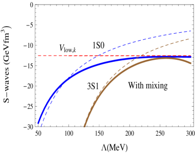
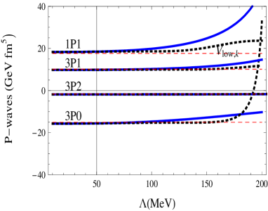
Figure 1: (Color on-line) Counterterms for the S- (in ${\rm MeV}{\rm fm}^{3}$, upper panel) and P-waves (${\rm MeV}{\rm fm}^{5}$, lower panel) as a function of the momentum scale $\Lambda$ (in MeV). C’s from Eqs. (9) solving Eqs. (6) including the D’s using just the low energy threshold parameters from Ref. Pavon Valderrama and Arriola (2005) (Thick Solid). C’s extracted from the diagonal $V_{\rm lowk}(p,p)$ potentials Bogner et al. (2003b) at fixed $\Lambda=420{\rm MeV}$ for the Argonne-V18 Wiringa et al. (1995) (dashed). C’s for P-waves including D-terms without mixings (thick dotted).

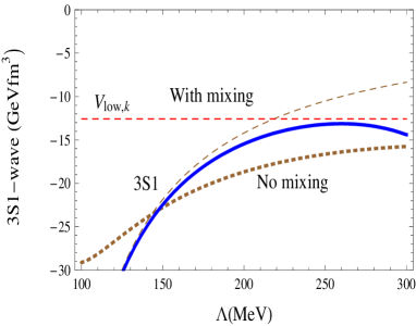
Figure 2: (Color on-line) $S-D$ waves mixing on $C_{{}^{3}S_{1}}$ (in ${\rm MeV}{\rm fm}^{3}$) as a function of the momentum space cut-off $\Lambda$ (in MeV) in the ${}^{3}S_{1}$ channel. We compare when including a) only $C_{{}^{3}S_{1}}$ (dashed), b) $C_{{}^{3}S_{1}}$ and $D_{{}^{3}S_{1}}$ (dotted), c) $C_{{}^{3}S_{1}}$, $D_{{}^{3}S_{1}}$ and $D_{E_{1}}$ (solid). Wigner symmetry is displayed when the mixing is included. See also Fig. 1 and Eq. (7) in the main text.

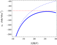
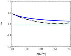
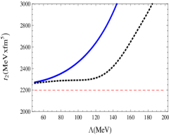
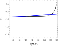
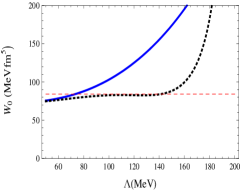
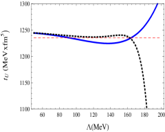
Figure 3: (Color on line) Skyrme force parameters as a function of the scale $\Lambda$ (in MeV). We compare with the Argonne-V18 Wiringa et al. (1995) exact $V_{\rm lowk}$ values evaluated at $\Lambda=420{\rm MeV}$ Bogner et al. (2003b). See also Fig. 1 and main text.

The corresponding T-matrices are conveniently solved by factoring out the centrifugal terms

$$T_{l^{\prime},l}(k^{\prime},k)=k^{l}k^{\prime l^{\prime}}\left[t_{l^{\prime},l}^{J}(p)+u_{l^{\prime},l}(p)(k^{2}+k^{\prime 2})+\dots\right]$$ (11)

which reduce the LS equation to a finite set of algebraic equations which are analytically solvable (see e.g. Ref. Entem et al. (2008) and references therein). In the simplest case where only the $C^{\prime}s$ are taken into account the explicit solutions for S- and P-waves are,

$$C_{S}(\Lambda) = \frac{16\pi^{2}\alpha_{0}}{M_{N}(1-2\alpha_{0}\Lambda/\pi)}\,,$$

$$C_{P}(\Lambda) = \frac{16\pi^{2}\alpha_{1}}{M_{N}(1-2\alpha_{1}\Lambda^{3}/3\pi)}\,,$$ (12)

where $\alpha_{0}$($\alpha_{1}$) is the scattering length (volume) defined by Eq. (5). The Eq. (12) illustrates the difference between a Fermi pseudo-potential and a coarse grained potential as the former corresponds to $\alpha_{0}\Lambda\ll 1$ where $C_{S}(\Lambda)\sim 16\pi^{2}\alpha_{0}/M_{N}$. In the case $\alpha_{0}\Lambda\gg 1$ one has instead $C_{S}(\Lambda)\sim-8\pi/(M\Lambda)$. Full solutions including the $D$’s are also analytical although a bit messier, so we do not display them explicitly. They rely on Eq. (4) with $\alpha_{{}^{1}S_{0}}$, $\alpha_{{}^{3}S_{1}}$, $\alpha_{{}^{3}P_{0}}$, $\alpha_{{}^{3}P_{1}}$, $\alpha_{{}^{3}P_{2}}$, $\alpha_{{}^{1}P_{1}}$, $\alpha_{E_{1}}$, $r_{{}^{3}S_{1}}$ and $r_{{}^{1}S_{0}}$ (see Ref. Pavon Valderrama and Arriola (2005) for numerical values for NijmII and Reid93 potentials). At the order considered here we just mention that while all P-waves constants run independently of each other with $\Lambda$ the spin-singlet parameters $C_{{}^{1}S_{0}}$, $D_{{}^{1}S_{0}}$ on the one hand and the spin-triplet parameters $C_{{}^{3}S_{1}}$, $D_{{}^{3}S_{1}}$ and $C_{E_{1}}$ on the other are intertwined.

We now turn to our numerical results. As can be seen from Fig. 1 the comparison of contact interactions using threshold parameters with $V_{\rm lowk}$ results evolved to $\Lambda=420{\rm MeV}$ Bogner et al. (2003b) (note the different normalization as ours) from the Argonne-V18 bare potential Wiringa et al. (1995) are saturated for $\Lambda=250{\rm MeV}$ for S-waves and for much lower cut-offs for P-waves. Note that this holds regardless on the details of the potential as we only need the low energy threshold parameters as determined e.g. in Ref. Pavon Valderrama and Arriola (2005). The strong dependence observed at larger $\Lambda$ values just reflects the inadequacy of the second order truncation in Eqs. (9). This also reflects in the $25\%-50\%$ inaccuracy are off the exact $V_{\rm lowk}$ of the D’s themselves despite showing plateaus, and thus will not be discussed any further.

The identity $C_{{}^{1}S_{0}}(\Lambda)=C_{{}^{3}S_{1}}(\Lambda)$ for $\Lambda\geq 250{\rm MeV}$ features the appearance of Wigner symmetry as pointed out in Ref. Calle Cordon and Ruiz Arriola (2008), but now we see that this does not depend on details of the force. Actually, the effect of the ${}^{3}S_{1}-^{3}D_{1}$wave mixing represented by a non-vanishing off diagonal potential $V_{E_{1}}(p^{\prime},p)$ becomes essential to achieve this identity (a fact disregarded in Ref. Mehen et al. (1999)). As can be seen from Fig. 2 there is a large mismatch at values of $\Lambda\sim 200-300{\rm MeV}$ when $D_{E_{1}}$ is set to zero (and hence $\alpha_{E_{1}}=0$) as compared with the case $D_{E_{1}}\neq 0$.

The scale dependence of the Skyrme interaction parameters (not involving the D’s) can be seen in Fig. 3 in comparison with the $V_{\rm lowk}$ potentials Bogner et al. (2003b) deduced from the Argonne-V18 bare potentials Wiringa et al. (1995). The plateaus observed in the different partial waves are corroborated here as well as a remarkable accuracy in reproducing the exact $V_{\rm lowk}$ numbers. Moreover, the weak cut-off dependence of the spin orbit interaction observed in Fig. 3 suggests taking $\Lambda\to 0$ in which case

$$W_{0}=\frac{\pi}{2M_{N}}\left(2\alpha_{{}^{3}P_{0}}+3\alpha_{{}^{3}P_{1}}-5\alpha_{{}^{3}P_{2}}\right)\,,$$ (13)

which upon using Ref. Pavon Valderrama and Arriola (2005) yields $W_{0}=72{\rm MeVfm}^{4}$. This numerical value reproduces within less than $10\%$ the exact $V_{\rm lowk}$ value. As can be seen from Fig. 3 the effective range correction $r_{1}$ provides via additional $D$ coefficients the missing contribution. This is a bit lower than what it is found in phenomenological approaches from the $p_{3/2}-p_{1/2}$ level splitting in ¹⁶O Bender et al. (2003). In any case, the comparison with phenomenological approaches based on mean field calculations may be tricky since as already mentioned not all the terms are always kept, and selective fits to finite nuclear properties may overemphasize the role played by specific terms.

It has recently been argued that counterterms are fingerprints of long distance symmetries Calle Cordon and Ruiz Arriola (2008, 2009); Ruiz Arriola and Calle Cordon (2009). This remarkable result holds regardless on the nature of the forces and applies in particular to both Wigner and Serber symmetries. We confirm that to great accuracy, $x_{0}=0$ (Wigner symmetry) and $x_{2}=-1$ (Serber symmetry). The astonishing large-$N_{c}$ ($N_{c}$ is the number of colours in QCD) relations discussed in Refs. Calle Cordon and Ruiz Arriola (2008, 2009); Ruiz Arriola and Calle Cordon (2009); Arriola and Cordon (2010) provide a direct link to the underlying quark and gluon dynamics and after Kaplan and Manohar (1997) suggests a $1/N_{c}^{2}$ accuracy of the Wigner symmetry in even-L partial waves. Wigner symmetry has proven crucial in Nuclear coarse lattice ($a\sim 2{\rm fm}$) calculations Lee (2009) in sidestepping the sign problem for fermions. As we see for the scales typically involved there this works with great accuracy already at $\Lambda\sim 250{\rm MeV}$. Taking into account that we deal with low energies, it is thus puzzling that Chiral interactions to N³LO Entem and Machleidt (2003) having chiral cut-offs $\Lambda_{\chi}\sim 600{\rm MeV}$ tend to violate Wigner symmetry in the $V_{\rm lowk}$ sense, i.e. $C_{{}^{1}S_{0}}^{\chi}\neq C_{{}^{3}S_{1}}^{\chi}$, whereas smaller values $\Lambda_{\chi}\sim 450{\rm MeV}$ Calle Cordon and Ruiz Arriola (2009) are preferred.

Within the low energy expansion we have neglected terms ${\cal O}({\bf p^{\prime}}^{4},{\bf p}^{4},{\bf p^{\prime}}^{2}{\bf p}^{2})$ which correspond to P-waves and S-wave range corrections. In configuration space this corresponds to a dimensional expansion, since $\delta(\vec{r}_{12})={\cal O}(\Lambda^{3})$ and $\{P^{2},\delta(\vec{r}_{12})\}={\cal O}(\Lambda^{5})$, $\{P^{4},\delta(\vec{r}_{12})\}={\cal O}(\Lambda^{7})$. Within such a scheme going to higher orders requires also to include three-body interactions, $\sim\delta(r_{12})\delta(r_{13})={\cal O}(\Lambda^{6})$. Actually, at the two body level there are more potential parameters than low energy threshold parameters. For instance, in the ${}^{1}S_{0}$ channel one has two independent hermitean operators, ${\bf p^{\prime}}^{4}+{\bf p}^{4}$ and $2{\bf p^{\prime}}^{2}{\bf p}^{2}$ (which are on-shell equivalent), but only one $v_{{}^{1}S_{0}}$ threshold parameter in the low energy expansion (see Eq. (4)). As it was shown in Ref. Amghar and Desplanques (1995) (see also Ref. Furnstahl et al. (2001)) these two features are interrelated since this two body off-shell ambiguity is cancelled when a three body observable, like e.g. the triton binding energy, is fixed . An intriguing aspect of the present investigation is the modification induced by potential tails due to e.g. pion exchange which cannot be represented by a polynomial since particle exchange generates a cut in the complex energy plane. The important issue, however, is that the low scale saturation unveiled in the present paper works accurately just to second order as long as the low energy parameters determined from on-shell scattering are properly reproduced.

I thank M. Pavón Valderrama and L.L. Salcedo for a critical reading of the ms and Jesús Navarro, A. Calle Cordón, T. Frederico and V.S. Timoteo for discussions. Work supported by the Spanish DGI and FEDER funds with grant FIS2008-01143/FIS, Junta de Andalucía grant FQM225-05.

References

- Moshinsky (1958) M. Moshinsky, Nuclear Physics 8, 19 (1958).
- Skyrme (1959) T. Skyrme, Nucl. Phys. 9, 615 (1959).
- Vautherin and Brink (1972) D. Vautherin and D. M. Brink, Phys. Rev. C5, 626 (1972).
- Negele and Vautherin (1972) J. W. Negele and D. Vautherin, Phys. Rev. C5, 1472 (1972).
- Chabanat et al. (1997) E. Chabanat, J. Meyer, P. Bonche, R. Schaeffer, and P. Haensel, Nucl. Phys. A627, 710 (1997).
- Bender et al. (2003) M. Bender, P.-H. Heenen, and P.-G. Reinhard, Rev. Mod. PHys. 75, 121 (2003).
- Moszkowski and Scott (1960) S. A. Moszkowski and B. L. Scott, Annals of Physics 11, 65 (1960).
- Dean et al. (2004) D. J. Dean, T. Engeland, M. Hjorth-Jensen, M. Kartamyshev, and E. Osnes, Prog. Part. Nucl. Phys. 53, 419 (2004), eprint nucl-th/0405034.
- Coraggio et al. (2009) L. Coraggio, A. Covello, A. Gargano, N. Itaco, and T. T. S. Kuo, Prog. Part. Nucl. Phys. 62, 135 (2009), eprint 0809.2144.
- Friedrich and Reinhard (1986) J. Friedrich and P. G. Reinhard, Phys. Rev. C33, 335 (1986).
- Klupfel et al. (2009) P. Klupfel, P. G. Reinhard, T. J. Burvenich, and J. A. Maruhn, Phys. Rev. C79, 034310 (2009), eprint 0804.3385.
- Furnstahl and Hackworth (1997) R. J. Furnstahl and J. C. Hackworth, Phys. Rev. C56, 2875 (1997), eprint nucl-th/9708018.
- Kortelainen et al. (2010) M. Kortelainen, R. J. Furnstahl, W. Nazarewicz, and M. V. Stoitsov (2010), eprint 1005.2552.
- Baldo et al. (2010) M. Baldo, L. Robledo, P. Schuck, and X. Vinas, J. Phys. G37, 064015 (2010), eprint 1005.1810.
- Stoitsov et al. (2010) M. Stoitsov et al. (2010), eprint 1009.3452.
- Bogner et al. (2003a) S. K. Bogner, T. T. S. Kuo, A. Schwenk, D. R. Entem, and R. Machleidt, Phys. Lett. B576, 265 (2003a), eprint nucl-th/0108041.
- Bogner et al. (2010) S. K. Bogner, R. J. Furnstahl, and A. Schwenk, Prog. Part. Nucl. Phys. 65, 94 (2010), eprint 0912.3688.
- Lee (2009) D. Lee, Prog. Part. Nucl. Phys. 63, 117 (2009), eprint 0804.3501.
- Calle Cordon and Ruiz Arriola (2008) A. Calle Cordon and E. Ruiz Arriola, Phys. Rev. C78, 054002 (2008), eprint 0807.2918.
- Calle Cordon and Ruiz Arriola (2009) A. Calle Cordon and E. Ruiz Arriola, Phys. Rev. C80, 014002 (2009), eprint 0904.0421.
- Ruiz Arriola and Calle Cordon (2009) E. Ruiz Arriola and A. Calle Cordon, PoS EFT09, 046 (2009), eprint 0904.4132.
- Arriola and Cordon (2010) E. R. Arriola and A. C. Cordon (2010), eprint 1009.3149.
- de la Plata and Salcedo (1998) M. J. de la Plata and L. L. Salcedo, J. Phys. A31, 4021 (1998), eprint hep-th/9609103.
- Bogner et al. (2003b) S. K. Bogner, T. T. S. Kuo, and A. Schwenk, Phys. Rept. 386, 1 (2003b), eprint nucl-th/0305035.
- Pavon Valderrama and Arriola (2005) M. Pavon Valderrama and E. R. Arriola, Phys. Rev. C72, 044007 (2005).
- Stoks et al. (1994) V. G. J. Stoks, R. A. M. Klomp, C. P. F. Terheggen, and J. J. de Swart, Phys. Rev. C49, 2950 (1994), eprint nucl-th/9406039.
- Holt et al. (2004) J. D. Holt, T. T. S. Kuo, G. E. Brown, and S. K. Bogner, Nucl. Phys. A733, 153 (2004), eprint nucl-th/0308036.
- Erkelenz et al. (1971) K. Erkelenz, R. Alzetta, and K. Holinde, Nuclear Physics A 176, 413 (1971).
- Epelbaum et al. (2000) E. Epelbaum, W. Gloeckle, and U.-G. Meissner, Nucl. Phys. A671, 295 (2000), eprint nucl-th/9910064.
- Wiringa et al. (1995) R. B. Wiringa, V. G. J. Stoks, and R. Schiavilla, Phys. Rev. C51, 38 (1995), eprint nucl-th/9408016.
- Entem et al. (2008) D. R. Entem, E. Ruiz Arriola, M. Pavon Valderrama, and R. Machleidt, Phys. Rev. C77, 044006 (2008), eprint 0709.2770.
- Mehen et al. (1999) T. Mehen, I. W. Stewart, and M. B. Wise, Phys. Rev. Lett. 83, 931 (1999), eprint hep-ph/9902370.
- Entem and Machleidt (2003) D. R. Entem and R. Machleidt, Phys. Rev. C68, 041001 (2003), eprint nucl-th/0304018.
- Kaplan and Manohar (1997) D. B. Kaplan and A. V. Manohar, Phys. Rev. C56, 76 (1997), eprint nucl-th/9612021.
- Amghar and Desplanques (1995) A. Amghar and B. Desplanques, Nucl. Phys. A585, 657 (1995).
- Furnstahl et al. (2001) R. J. Furnstahl, H. W. Hammer, and N. Tirfessa, Nucl. Phys. A689, 846 (2001), eprint nucl-th/0010078.