Generation of longitudinal flux tube waves in
theoretical main-sequence stars:
Effects of model parameters

Abstract

Context. Continued investigation of the linkage between magneto-acoustic energy generation in stellar convective zones and the energy dissipation and radiative emission in outer stellar atmospheres in stars of different activity levels.

Aims. We compute the wave energy fluxes carried by longitudinal tube waves along vertically oriented thin magnetic fluxes tubes embedded in the atmospheres of theoretical main-sequence stars based on stellar parameters deduced by R. L. Kurucz and D. F. Gray. Additionally, we present a fitting formula for the wave energy flux based on the governing stellar and magnetic parameters.

Methods. A modified theory of turbulence generation based on the mixing-length concept is combined with the magneto-hydrodynamic equations to numerically account for the wave energies generated at the base of magnetic flux tubes.

Results. The results indicate a stiff dependence of the generated wave energy on the stellar and magnetic parameters in principal agreement with previous studies. The wave energy flux $F_{\rm LTW}$ decreases by about a factor of 1.7 between G0 V and K0 V stars, but drops by almost two orders of magnitude between K0 V and M0 V stars. In addition, the values for $F_{\rm LTW}$ are significantly higher for lower in-tube magnetic field strengths. Both results are consistent with the findings from previous studies.

Conclusions. Our study will add to the description of magnetic energy generation in late-type main-sequence stars. Our results will be helpful for calculating theoretical atmospheric models for stars of different levels of magnetic activity.

1 Introduction

An outstanding problem in stellar astrophysics concerns the identification of physical processes responsible for the heating of outer stellar atmospheres and the acceleration of stellar winds (see reviews by Narain & Ulmschneider 1990, 1996 and Güdel 2007). For the Sun and other types of stars with surface convection zones, acoustic heating has been identified as most likely responsible for balancing the “basal” flux emission (e.g., Buchholz et al. 1998; Cuntz et al. 2007). On the other hand, it is well known that most, if not all stars also exhibit a large amount of magnetic activity. Thus, the chromospheres of main-sequence stars, including the Sun, are expected to be significantly shaped by magnetically heated structure (e.g., Saar 1994; Schrijver 1996).

There is a large body of previous work devoted to the description of the two-component structure of stellar chromospheres. In these models the magnetic component of the chromosphere is typically heated by energy dissipation of longitudinal flux tube waves. Cuntz et al. (1999) computed two-component theoretical chromosphere models for K2 V stars with different levels of magnetic activity with the filling factor for the magnetic component determined from an observational relationship between the measured magnetic area coverage and the stellar rotation period. For stars with very slow rotation, they were able to reproduce the basal flux limit of chromospheric emission previously identified with non-magnetic regions. Most notably, however, Cuntz et al. (1999) deduced a relationship between the Ca II H+K emission and the stellar rotation rate that is consistent with the relationship previously obtained by observations; see also Cuntz et al. (1998) for earlier results.

Further studies for a large spectral range of stars were given by Fawzy et al. (2002) based on specified values for the magnetic filling factor. They concluded that heating by acoustic and longitudinal flux tube waves is able to explain most of the observed range of chromospheric activity as gauged by the Ca II and Mg II lines. On the other hand, indirect evidence for non-wave (i.e., reconnective) heating was also deduced needed to explain the structure of the highest layers of stellar chromospheres.

This type of models, as well as envisioned future models of chromospheric heating and emission, partially motivated by the quest of investigating the effects of UV and EUV emission on planetary atmosphere and (potentially) the evolution of life (e.g., Guinan et al. 2003; Lammer et al. 2003; Güdel 2007; Cuntz et al. 2010), require the continuation of detailed simulations of magnetic wave energy generation, including studies on longitudinal tube waves in different types of stars, particularly main-sequence stars. This latter goal is the focus of the present paper.

Previous work on the calculation of longitudinal tube waves has been based on progress made by Musielak et al. (1994) who corrected the Lighthill-Stein theory by incorporating an improved description of the spatial and temporal spectrum of the turbulent convection and utilized the corrected theory for calculating revised stellar acoustic wave energy fluxes (Ulmschneider et al. 1996, 1999). This type of work focused on the generation of acoustic waves; however, it did not consider stellar magnetic fields. Considering the fundamental importance of magnetic heating in most, if not all stars, a set of papers focused on the study of longitudinal and transverse tube wave generation has been pursued (e.g. Musielak et al. 1989, 1995; Ulmschneider & Musielak 1998). In subsequent work, Ulmschneider et al. (2001) used the approach developed by Ulmschneider & Musielak (1998) to compute the wave energy fluxes carried by longitudinal tube waves propagating along thin and vertically oriented magnetic flux tubes that are embedded in atmospheres of late-type stars. This numerical approach supplemented previous work by Musielak et al. (2000), who analytically calculated the longitudinal wave energy fluxes generated in stellar convective zones.

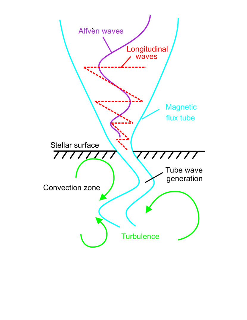
Figure 1: Diagram of a flux tube embedded into a stellar convective zone. The squeezing point of the tube is assumed to be located at optical depth $\tau_{5000}=1$, coinciding with the “stellar surface”. Credit: P. Ulmschneider.

In the numerical approach by Ulmschneider & Musielak (1998), longitudinal tube waves are generated as a result of the squeezing of a thin, vertically oriented magnetic flux tube by external pressure fluctuations produced by the turbulent motions in a stellar photosphere and convection zone, which correspond to associated velocity fluctuations. Hence, to compute the pressure fluctuations imposed on the tube, it is required to know the external turbulent motions. The motions are modeled by specifying the rms velocity amplitude and using an extended Kolmogorov turbulent energy spectrum with a modified Gaussian frequency factor (Musielak et al. 1994).

The main advantage of this approach is that it is not restricted to linear waves and that it allows for occasionally large-amplitude waves observed on the Sun at the photospheric level (e.g., Muller 1985; Komm et al. 1991; Nesis et al. 1993; Muller et al. 1994) and also seen in detailed time-dependent simulations of solar and stellar convection (e.g., Nordlund & Dravins 1990; Nordlund & Stein 1991; Cattaneo et al. 1991; Steffen 1993; Nordlund et al. 1997). Horizontal flow patterns are a notable candidate process for the initiation of wave modes with respect to flux tubes (see Fig. 1); see Stein et al. (2009a, b) for recent models of convective flows for the Sun based on up-to-date simulations extending toward the scale of supergranules.

The code used by Ulmschneider & Musielak (1998) was originally developed by Herbold et al. (1985) who treated magnetic flux tubes in the so-called thin flux tube approximation and described them mathematically by using a set of one-dimensional, time-dependent and nonlinear MHD equations. It allows to compute the instantaneous and time-averaged longitudinal tube wave energy fluxes and the corresponding wave energy spectra. It requires specifying the strength of the magnetic field inside the flux tube and the height in the stellar atmosphere where the squeezing is assumed to take place. The code has previously been used to calculate wave energy fluxes and spectra for longitudinal tube waves propagating in the solar atmosphere (see Fawzy et al. 1998 for models of different spreading factors), and to investigate the dependence of these fluxes on the magnetic field strength, the rms velocity amplitude of turbulent motions, and the location of the squeezing in the atmosphere; for recent models for other stars with non-solar metallicities see Fawzy (2010).

The reason for reinvestigating the generation of longitudinal flux tube waves in main-sequence stars is three-fold. First, we would like to use realistic combinations of ($T_{\rm eff}$, $\log g$), with $T_{\rm eff}$ as stellar effective temperature and $\log g$ as surface gravity, for main-sequence stars guided by up-to-date studies by R. L. Kurucz and D. F. Gray. Note that $\log g$ is typically close to 4.5 (see Table 1). Previous models by Ulmschneider et al. (2001) and others have been pursued for either $\log g=4$ or $5$, thus resulting in unnecessary interpolation errors. Secondly, we would like to investigate the amount of upward propagating longitudinal wave energy flux for a wider range of stellar convective and magnetic parameters, notably the mixing length $\alpha$ amid recent progress made through models by Stein et al. (2009a, b) and others. Thirdly, we would like to deduce a fitting formula for the wave energy flux that allows insight into the role of the relevant parameters concerning that flux and, furthermore, offers a more universal use.

Our paper is structured as follows: In Sect. 2, we comment on the parameters of theoretical main-sequence stars. Additionally, we summarize the method for the computation of longitudinal tube waves as well as the construction of stellar flux tube models. Our results are given in Sect. 3. Finally, in Sect. 4 we present the summary and conclusions.

Table 1: Theoretical main-sequence stars

Sp. Type	$T_{\rm eff}$	$R$	$M$	$\log\leavevmode\nobreak\ g$
…	(K)	($R_{\odot}$)	($M_{\odot}$)	…
F0 V	7178	1.620	1.600	4.223
F1 V	7042	1.541	1.560	4.255
F2 V	6909	1.480	1.520	4.279
F3 V	6780	1.453	1.480	4.283
F4 V	6653	1.427	1.440	4.287
F5 V	6528	1.400	1.400	4.292
F6 V	6403	1.333	1.330	4.312
F7 V	6280	1.267	1.260	4.333
F8 V	6160	1.200	1.190	4.355
F9 V	6047	1.155	1.120	4.362
G0 V	5943	1.120	1.050	4.360
G1 V	5872	1.100	1.022	4.364
G2 V	5811	1.080	0.994	4.368
G3 V	5760	1.037	0.967	4.392
G4 V	5708	0.993	0.940	4.417
G5 V	5657	0.950	0.914	4.443
G6 V	5603	0.937	0.888	4.443
G7 V	5546	0.923	0.863	4.443
G8 V	5486	0.910	0.838	4.443
G9 V	5388	0.870	0.814	4.469
K0 V	5282	0.830	0.790	4.497
K1 V	5169	0.790	0.766	4.527
K2 V	5055	0.750	0.742	4.558
K3 V	4973	0.730	0.718	4.567
K4 V	4730	0.685	0.694	4.608
K5 V	4487	0.640	0.670	4.651
K6 V	4294	0.601	0.643	4.689
K7 V	4133	0.565	0.614	4.722
K8 V	4006	0.533	0.582	4.749
K9 V	3911	0.505	0.547	4.770
M0 V	3850	0.480	0.510	4.783

2 Methods

2.1 Comments on the theoretical main-sequence stars

Stellar parameters for theoretical main-sequence stars have been deduced by Gray (2005); see his Table B.1. His values, notably $T_{\rm eff}$ and $\log g$, serve as basis for the present study. We also improved the accuracy of the $\log g$ values if more accurate values for the stellar masses and stellar radii were given. For stellar spectral types with no data given, we calculated those data using biparabolic interpolation. The stellar data are summarized in Table 1.

Another set of spectral models has been constructed by R. L. Kurucz and collaborators. They take into account millions or hundred of millions of lines for a large array of atoms and molecules; see, e.g., Castelli & Kurucz (2004) and Kurucz (2005) for technical details. These models indicate very similar effective temperatures compared to the models by Gray (2005) for most types of stars. However, stellar spectral types of K5 V and below, the indicated effective temperatures of R. L. Kurucz are consistently lower noting that the difference amounts to nearly 300 K for spectral type M0 V. Therefore, we assumed average values between the models by D. F. Gray and R. L. Kurucz for stars of spectral spectral type K5 V and M0 V in the following.

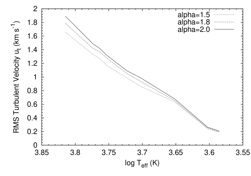
Figure 2: Root mean square turbulent velocities at the squeezing point ($\tau_{5000}=1$) for the set of theoretical main-sequence stars for different values of the mixing-length parameter $\alpha$.

Figure 3: Power spectra of the instantaneous wave energy flux in flux tubes with $B/B_{\rm eq}=0.85$ for F5 V, G5 V, K5 V, and M0 V stars (from top to bottom) as a function of circular frequency $\omega$. The mixing-length parameter is assumed as $\alpha=2$.

Table 2: Wave energy flux^a for different parameters $\alpha$ and $\eta$

Sp.Type	$T_{\rm eff}$	$F_{\rm LTW}$	$F_{\rm LTW}$	$F_{\rm LTW}$
…	(K)	…	…	…
…	…	$\eta=0.75$	$\eta=0.85$	$\eta=0.95$
$\alpha=1.5$
F5 V	6528	6.03E8	4.05E8	9.41E7
F8 V	6160	5.59E8	3.10E8	9.14E7
G0 V	5943	4.75E8	2.94E8	7.91E7
G2 V	5811	4.50E8	2.62E8	7.91E7
G5 V	5657	3.56E8	2.20E8	6.53E7
G8 V	5486	3.27E8	1.98E8	5.85E7
K0 V	5282	2.54E8	1.56E8	4.77E7
K2 V	5055	1.92E8	1.10E8	3.42E7
K5 V	4487	1.14E8	6.83E7	2.12E7
K8 V	4006	4.47E6	2.87E6	9.82E5
M0 V	3850	2.26E6	1.33E6	5.36E5
$\alpha=1.8$
F5 V	6528	8.99E8	5.00E8	1.25E8
F8 V	6160	7.51E8	4.62E8	1.15E8
G0 V	5943	5.69E8	3.40E8	9.73E7
G2 V	5811	5.63E8	3.02E8	9.05E7
G5 V	5657	5.29E8	2.78E8	7.96E7
G8 V	5486	3.98E8	2.37E8	7.32E7
K0 V	5282	2.93E8	1.82E8	5.60E7
K2 V	5055	2.69E8	1.63E8	4.72E7
K5 V	4487	1.30E8	8.15E7	2.50E7
K8 V	4006	5.36E6	3.50E6	1.24E6
M0 V	3850	2.28E6	1.44E6	6.49E5
$\alpha=2.0$
F5 V	6528	1.12E9	6.07E8	1.47E8
F8 V	6160	8.51E8	4.92E8	1.34E8
G0 V	5943	6.77E8	3.96E8	1.11E8
G2 V	5811	6.35E8	3.65E8	1.06E8
G5 V	5657	5.81E8	3.35E8	1.01E8
G8 V	5486	4.79E8	2.86E8	8.05E7
K0 V	5282	3.39E8	1.95E8	6.39E7
K2 V	5055	2.98E8	1.86E8	5.81E7
K5 V	4487	1.44E8	9.19E7	2.86E7
K8 V	4006	6.79E6	4.37E6	1.57E6
M0 V	3850	3.32E6	2.11E6	7.62E5

• ^aThe unit of $F_{\rm LTW}$ is erg cm^-2 s^-1.

2.2 Convective zone models and turbulent velocities

The method for calculating wave energy fluxes carried by longitudinal tube waves adopted in the present paper has been described in detail by Ulmschneider et al. (2001). Thus, it is not necessary to present an intricate discussion in the following. In the solar application, it is possible to select many model parameters and characteristic values directly from observations. However, for stars other than the Sun such data are mostly unavailable. Therefore, we need to discuss in some detail the physical reasoning behind our choice of relevant parameters used in our calculations.

In the current approach, the magnetic flux tubes are embedded in nonmagnetized photospheric convection zones (see Fig. 1). Considering that the interaction between the flux tubes and the convective turbulence is the driving mechanism for the generation of longitudinal tube waves, among other waves, models of the stellar convection zones are required. Guided by previous studies, it is assumed that the squeezing of the tube is symmetric with respect to the tube axis. The computed pressure fluctuations are subsequently translated into gas pressure and magnetic field fluctuations inside the tube assuming horizontal pressure balance. Finally, the internal velocity perturbation resulting from the internal pressure fluctuation is calculated. This internal velocity served as a boundary condition in the numerical simulation of the generation of the longitudinal tube waves.

Both numerical simulations of stellar convection and mixing length models show that the maximum convective velocities occur at optical depths of $\tau_{5000}\approx 10$ to 100. For example, Steffen (1993) found in his time-dependent solar numerical convection calculations that maximum convective velocities $v_{\rm CMax}\simeq 2.8$ km s^-1 are reached at $\tau_{5000}\approx 50$ and that these values can be reproduced via mixing length theory with a mixing length parameter of $\alpha\simeq 2$. The value $\alpha=2$ is furthermore indicated by time-dependent hydrodynamic simulations of stellar convection for stars other than the Sun (Trampedach et al. 1997) as well as by a careful fitting of evolutionary tracks of the Sun with its present luminosity, effective temperature and age (Schröder & Eggleton 1996).

Nevertheless, there is still some debate about the most appropriate value of $\alpha$. Nordlund & Dravins (1990) originally pursued detailed numerical simulations based on 3-D hydrodynamics coupled with 3-D non-grey radiative transfer for stars similar to Procyon (F5 IV-V), $\alpha$ Cen A (G2 V), $\beta$ Hyi (G2 IV), and $\alpha$ Cen B (K1 V). They concluded a mixing-length parameter of $\alpha=1.5$ (or slightly higher), although the mixing length concept appeared to be problematic at photospheric heights. A mixing length of 1.5 was also used by Cuntz et al. (1999) in their two-component theoretical chromosphere models for K2 V stars with different levels of magnetic activity. Even though the deduced relationship between the Ca II H+K emission and the stellar rotation rate was found to be largely consistent with the observed relationship, the agreement could probably be improved if a somewhat higher longitudinal wave energy flux, corresponding to a slightly larger mixing length parameter, was adopted. Recently, Stein et al. (2009a, b) pursued updated state-of-the-art simulations of solar convection zone extending toward the scale of supergranules indicating a mixing length parameter of $\alpha\simeq 1.8$. For these reasons, we will calculate a set of models concerning wave energy generation of longitudinal tube wave for a set of $\alpha$ values, which are $\alpha$ = 1.5, 1.8, and 2.0.

2.3 Computation of stellar magnetic flux tube models

Our treatment of stellar convection associated with the facilitation of stellar flux tube models is akin to that described by Ulmschneider et al. (1996). In this approach, information is needed about velocities of turbulent motions in the overshooting layer near the stellar surface, where the squeezing of the magnetic flux tube is assumed to occur. Steffen’s numerical calculations show that the rms velocities decrease toward the solar surface and reach a plateau in the overshooting layer. Between $\tau_{5000}=1$ and $10^{-4}$, he finds values of $v_{\rm rms}=1.4$ km s^-1, which are essentially independent of height. Ulmschneider & Musielak (1998) adopted for the Sun a variety of observed rms velocity amplitudes $u_{t}$ in the range $0.9<u_{t}<1.9$ km s^-1, and showed the dependence of the computed fluxes on this velocity. For stars, these velocities cannot be determined from observations; thus, we follow Ulmschneider et al. (2001) by assuming that the rms velocity fluctuations at the squeezing points are given by $u_{t}=v_{\rm CMax}/2$. The values of $v_{\rm t}$ and $v_{\rm CMax}$ (see Fig. 2) are evaluated from stellar convection zone models based on the adopted mixing length parameter. The numerical factor 2 used in our calculations ensures that in our approach the considered convective velocities are always lower than the local speed of sound.

After specifying the rms velocities that are responsible for the wave generation, we also determine the height in stellar atmospheres, where the most efficient squeezing of magnetic flux tubes takes place. We are guided by earlier studies performed by Ulmschneider & Musielak (1998), who pointed out that shifting the height of the excitation point did not change much the resulting wave energy fluxes for the Sun. Based on these results, we take the squeezing point to be located at optical depth $\tau_{5000}=1$ for all considered stars. This depth is commonly taken as the zero height level in stellar atmosphere computations.

Table 3: Wave energy flux^a for different values of $\eta$ based on $\alpha=2$

Sp.Type	$T_{\rm eff}$	$F$(tot)	$F$(prop)	$F$(prop+up)	$F$(tot)	$F$(prop)	$F$(prop+up)	$F$(tot)	$F$(prop)	$F$(prop+up)
…	(K)	…	…	…	…	…	…	…	…	…
…	…	$\eta=0.75$			$\eta=0.85$			$\eta=0.95$
F2 V	6909	…	…	…	5.18E8	4.37E8	6.26E8	1.17E8	1.01E8	1.41E8
F5 V	6528	8.23E8	6.97E8	1.12E9	5.04E8	4.13E8	6.07E8	1.27E8	1.08E8	1.47E8
F8 V	6160	6.76E8	6.02E8	8.51E8	4.10E8	3.59E8	4.92E8	1.09E8	9.48E7	1.34E8
G0 V	5943	5.45E8	4.71E8	6.77E8	3.22E8	2.76E8	3.96E8	9.75E7	8.11E7	1.11E8
G2 V	5811	4.91E8	4.26E8	6.35E8	2.96E8	2.53E8	3.65E8	8.70E7	7.56E7	1.06E8
G5 V	5657	4.75E8	3.93E8	5.81E8	2.73E8	2.32E8	3.35E8	8.45E7	7.22E7	1.01E8
G8 V	5486	3.86E8	3.29E8	4.79E8	2.38E8	2.02E8	2.86E8	6.76E7	5.87E7	8.05E7
K0 V	5282	2.95E8	2.30E8	3.39E8	1.66E8	1.39E8	1.95E8	5.47E7	4.68E7	6.39E7
K2 V	5055	2.52E8	2.08E8	2.98E8	1.55E8	1.26E8	1.86E8	4.86E7	3.90E7	5.81E7
K5 V	4487	1.29E8	8.93E7	1.44E8	8.08E7	5.93E7	9.19E7	2.53E7	1.83E7	2.86E7
K8 V	4006	5.55E6	3.36E6	6.79E6	3.74E6	2.14E6	4.37E6	1.25E6	6.95E5	1.57E6
M0 V	3850	2.29E6	1.36E6	3.32E6	1.57E6	8.23E5	2.11E6	5.37E5	2.86E5	7.62E5

• ^aThe unit of $F$(tot), $F$(prop), and $F$(prop+up) is erg cm^-2 s^-1. Note that $F$(prop+up) $\equiv$ $F_{\rm LTW}$.

For the computation of stellar magnetic flux tubes we consider the “thin flux tube approximation” (e.g., Spruit 1981). Two dimensional modeling of magnetic flux tubes by Hasan et al. (2003) indicates that this approach renders reasonable results if the models do not extend beyond a small number of scale heights above the stellar surface; note that this approximation is fully compatible with our study. In the following, we augment the commonly used concept of solar magnetic flux tubes (e.g., Stenflo 1978; Solanki 1993) to stellar flux tubes; see Solanki (1996) for further discussion. Stellar magnetic flux tubes at the stellar surface are assumed to have diameters of roughly equal to the local pressure scale height like in case of the Sun.

For the Sun, the magnetic flux tubes within the solar photosphere have field strengths on the order $B_{0}=1500$ G (e.g., Solanki 1993). Taking $p_{e}=1.17\cdot 10^{5}\ \rm dyn\ cm^{-2}$ from model C of Vernazza et al. (1981) at the height $z=0$ where $\tau_{5000}=1$ yields an equipartition field strength ($B_{\rm eq}^{2}/8\pi=p_{e}$) of $B_{\rm eq}=1716$ G. This corresponds to a ratio $B/B_{\rm eq}=0.875$, which may or may not be typical for stellar flux tubes. Since this ratio is likely to vary even on the Sun (e.g., Schrijver & Zwaan 2000), it is appropriate to consider a range of that ratio for the sake of comprehensiveness. Therefore, we take $B/B_{\rm eq}=0.75$, 0.85, and 0.95 for our stellar flux tube models. This allows us to deduce an appropriate set of energy fluxes for upward propagating longitudinal tube waves for specified values of $\alpha=1.5$, 1.8, and 2.0, resulting in a total of 9 models per theoretical target star.

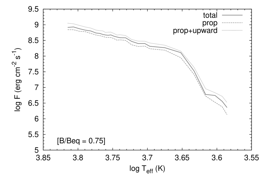
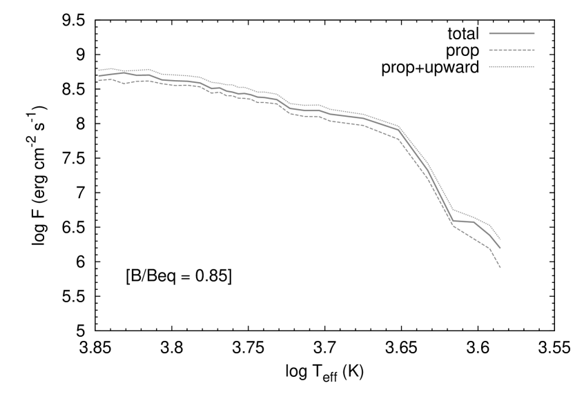
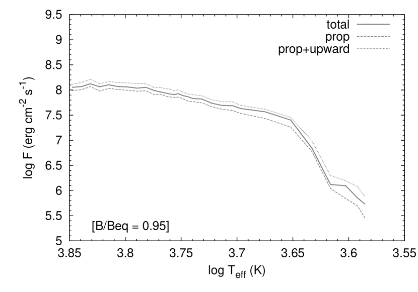
Figure 4: Different types of energy fluxes (see text) for the set of theoretical main-sequence stars for $\alpha=2$. Results are given for $B/B_{\rm eq}=0.75$ (top), 0.85 (middle), and 0.95 (bottom).

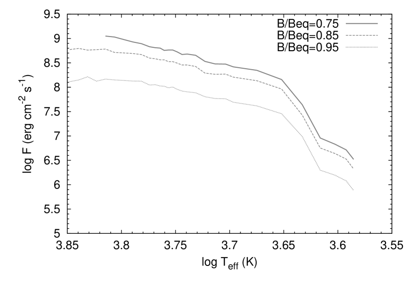
Figure 5: Upward propagating energy fluxes, also referred to as $F_{\rm LTW}$, for the set of theoretical main-sequence stars for $\alpha=2$ and different values of $\eta=B/B_{\rm eq}$.

3 Results and discussion

3.1 Computation of wave energy fluxes

The instantaneous and time-averaged tube wave energy fluxes are computed by employing a modified time-dependent wave code based on an earlier version by Herbold et al. (1985). The external turbulent motion is translated into internal pressure and velocity fluctuations. The time-averaged wave energy fluxes at the squeezing point are computed for each combination of effective temperature $T_{\rm eff}$, surface gravity $\log g$, $\eta=B/B_{\rm eq}$ and mixing-length parameter $\alpha$ for flux tubes embedded in the atmospheres of the main-sequence stars as considered.

For the evaluation of reliable time-averaged wave energy fluxes and due to the spiky nature of the instantaneous wave energy fluxes, the wave propagation code has to be run over a time of about $35P_{D}$ with $P_{D}$ as the wave period of the Defouw cut-off frequency (Defouw 1976). The generated waves include both propagating and non-propagating wave energy fluxes. We apply a high pass filter at the Defouw cut-off frequency, $\omega_{D}$, on the velocity and pressure fluctuations inside the flux tubes to separate the propagating waves and to compute the time-averaged upward propagating wave components. The position of the filter is indicated by the low frequency cut-off depicted in Fig. 3, which features a comparison of the power spectra for different types of stars. Note that the power spectra reach their maxima at roughly $2\omega_{D}$ and decrease toward higher frequencies.

Figure 4 and 5 as well as Table 2 and 3 show the computed wave energy of the magnetic flux tube. Actually, Table 3 for the case of $\alpha=2$ also distinguishes between the total energy flux, propagating energy flux and upward propagating energy flux; see Ulmschneider et al. (2001) for detailed definitions. The wave energy flux $F_{\rm LTW}$ identified as upward propagating energy flux shows a characteristic behaviour as function of the model parameters, notably the stellar spectral type (or $T_{\rm eff}$). It is found that the value of $F_{\rm LTW}$ decreases by about a factor of 1.7 between G0 V and K0 V stars, and drops by almost two orders of magnitude between K0 V and M0 V stars. This is a direct consequence of the action of stellar convection, noting that in relatively hot main-sequence stars there is an enhanced efficiency in the creation of turbulence, reflected in higher values of the rms velocity $u_{t}$ (see Fig. 2).

Additionally, we also found that the wave energy flux $F_{\rm LTW}$ shows significant dependence on the magnetic field strengths inside of the tubes, given as $\eta=B/B_{\rm eq}$ as well as some minor dependence on the mixing-length parameter $\alpha$. In fact, the wave energy fluxes are found to increase with decreasing magnetic field strengths inside the flux tube, a phenomenon that can be explained by the decreasing stiffness of the magnetic tube; see Fig. 5 for details. This behaviour was previously also pointed out by Ulmschneider et al. (2001).

Moreover, it is found that the wave energy flux for upward propagating waves is also somewhat sensitive to the choice of $\alpha$ concerning the stellar convective zone. Note that an increase of the mixing length from $\alpha$ = 1.5 to 2.0 amplifies the simulated longitudinal wave energy fluxes by a factor of approximately 1.45, which is most notable for relatively hot main-sequence stars. This can be explained by the fact that for higher values of $\alpha$, the convective zones are more efficient concerning the generation of turbulence, thus resulting in thus higher values of the rms velocity $u_{t}$ (see Fig. 2).

3.2 Derivation of fitting formulas

The amount of data for $F_{\rm LTW}$ for stars of different spectral types and the various choices for $\eta$ and the mixing-length parameter $\alpha$ are a strong motivation for the derivation of a fitting formulas. Our main focus are stars between $T_{\rm eff}=6000$ K (i.e., spectral type F9.5 V) and stars of spectral-type mid-K. Stars below mid-K are increasingly dominated by flare activity or other processes as, e.g., magnetic reconnection (e.g., Narain & Ulmschneider 1996), which makes the existence of an accurate fitting formula less urgent. Nevertheless, we extended our fitting formula toward stars of spectral type M0 V (with $T_{\rm eff}=3850$ K) while reproducing the wave energy flux of M0 V stars with a precision of 10^-3.

However, no attempt has been made to accurately reproduce the knee in the wave energy flux function near F8 V as this would have led to an additional complication in our fitting formula without obvious merits. This approach is motivated by the finding that energy dissipation by longitudinal tube waves appears to be less important in dwarfs stars of spectal type mid-K to M compared to, e.g., flare heating as pointed out by Fawzy et al. (2002) in their comparison between empirical and theoretical radiative chromospheric emission losses.

Our formula is given as follows:

$$F_{\rm LTW}\ =\ 2.55\cdot 10^{8}\ T_{\rm rel}^{\epsilon}\ e^{{\mu}T_{\rm dif}}\ Z(\alpha,\eta)\ \ {\rm erg\leavevmode\nobreak\ cm}^{-2}\leavevmode\nobreak\ {\rm s}^{-1}$$ (1)

with $T_{\rm rel}=T_{\rm eff}/T_{{\rm eff},\odot}$ noting that $T_{{\rm eff},\odot}=5777$ K. In addition, $Z(\alpha,\eta)$ is given as

$$Z(\alpha,\eta)\ =\ \alpha^{1.25}\cdot\Bigl{(}{\eta\over 0.75}\Bigr{)}^{\gamma}$$ (2)

with $\eta=B/B_{\rm eq}$ and $\gamma=-4.5-30\cdot|\eta-0.85|$. Furthermore, $T_{\rm dif}$ is defined as Min$(0,T_{\rm eff}-4500$ K), which means that $T_{\rm dif}$ is zero for $T_{\rm eff}\geq 4500\leavevmode\nobreak\ {\rm K}$ and takes a negative value otherwise. Note that the parameters $\epsilon$ and $\mu$ of Eq. (1) weakly depend on $\alpha$ and $\eta$; see Table 4 and 5 for detailed information. If a reduced level of accuracy is permitted, it might be appropriate to use average values for $\alpha$ and $\mu$, given as $\alpha=5.21$ and $\mu=4.66\cdot 10^{-3}$, respectively.

Our formula for the upward propagating longitudinal wave energy flux has been subjected to thorough testing for stars of spectral type F9.5 V, G2 V, G5 V, G8 V, K0 V, K2 V, and K5 V. The simulated data for the F9.5 V star were obtained via logarithmic interpolation between the data for the F8 V and G0 V stars. Detailed information on the tests is given in Appendix A.

Table 4: Data for the parameter $\epsilon$

$\alpha$	$\eta=0.75$	$\eta=0.85$	$\eta=0.95$
1.5	5.24	5.30	4.95
1.8	5.51	5.11	4.87
2.0	5.67	5.31	4.90

Table 5: Data for the parameter $\mu$

$\alpha$	$\eta=0.75$	$\eta=0.85$	$\eta=0.95$
1.5	4.78E-3	4.69E-3	4.45E-3
1.8	4.95E-3	5.04E-3	4.55E-3
2.0	4.47E-3	4.53E-3	4.49E-3

4 Summary and conclusions

We studied the generation of longitudinal waves in stellar magnetic flux tubes of theoretical main-sequence stars. Our results are commensurate with those obtained from previous studies, especially the work by Ulmschneider et al. (2001). Our investigations show that through nonlinear time-dependent responses of stellar magnetic flux tubes to continuous and impulsive external turbulent pressure fluctuations, longitudinal tube waves were effectively produced via dipole emission. Furthermore, the shapes of the computed power spectra were found to be similar for stars of different effective temperature. Moreover, the longitudinal wave energy fluxes are found to increase with higher effective temperature, i.e., stars of earlier spectral types.

As part of our study, we investigated the role of the magnetic field strength inside of the tube $B$ as well as that of the adopted convective model characterized by the mixing-length parameter $\alpha$ concerning the generated wave energy flux. We found that the computed wave energy flux strongly depends on the strength of the magnetic field as already discussed in previous studies (e.g., Ulmschneider & Musielak 1998; Ulmschneider et al. 2001). For a given spectral type, the flux is considerably higher in tubes with a field strength of $B/B_{\rm eq}=0.75$ compared to $B/B_{\rm eq}=0.95$, although the difference as a function of spectral type is not as large as previously pointed out by Ulmschneider et al. (2001) owing to the differences in stellar surface gravity for the different types of stars. Note that the difference concerning the magnetic field strength of $B/B_{\rm eq}=0.75$ and 0.95 is found to be a factor of 7.6, 6.1, 5.3, and 4.4 (for $\alpha=2$) for stars of spectral type F5 V, G0 V, K0 V, and M0 V, respectively. This difference exhibits a noticeable, albeit little dependence on the mixing-length parameter $\alpha$ for stars hotter than G2 V, rooted in the behaviour of the adopted root mean square velocity at the squeezing point of the tube.

Another aspect of our study was to consider a limited range of the mixing-length parameter $\alpha$, which are 1.5, 1.8, and 2.0. It was found that an increase of the mixing length from $\alpha$ = 1.5 to 2.0 enhances the computed energy fluxes by a factor of about 1.45, corresponding to a proportionality of $\alpha^{1.25}$. This relationship can be compared with previous findings for acoustic energy generation, which show a dependence such as $\alpha^{2.8}$ (Bohn 1984) or $\alpha^{3.8}$ in updated models by Musielak et al. (1994). The relatively weak influence of $\alpha$ on the amount of upward propagating wave energy flux $F_{\rm LTW}$ is apparently due to the fact that the latter is largely controlled by magnetic processes, as also evidenced by the strong influence of $\eta$ up to $\eta^{-7.5}$, rather than controlled by convective processes, even though the latter are key for the excitement of the tubes subsequently resulting in magnetic wave generation.

Note that the strong dependence of the generated wave energy fluxes on the stellar and magnetic parameters is in general agreement with the findings from previous studies, although some noticeable differences are attained. The wave energy flux $F_{\rm LTW}$ decreases by about a factor of 1.7 between the G0 V and K0 V stars, and drops by almost two orders of magnitude between the K0 V and M0 V stars. For $\alpha=2$ at a fixed value of $T_{\rm eff}=5000$ K, Ulmschneider et al. (2001) deduced a fitting formula for the behaviour of $F_{\rm LTW}$ as function of $B/B_{\rm eq}$, which is found to be commensurate with the results obtained in our current study. On the other hand, the fitting formula for the wave energy flux given in our paper is more general than any of the previously deduced formulas as it is applicable to a large range of stellar effective temperatures and furthermore allows insight into the role of the governing magnetic and convective parameters concerning the amount of generated upward propagating wave energy flux. Therefore, it is of interest to future solar and stellar physics studies as it allows flexibility both concerning the mixing-length parameter $\alpha$ and the magnetic parameter $\eta=B/B_{\rm eq}$. Note that even for the Sun, $\eta$ is expected to exhibit considerable spatial and temporal fluctuations across the surface as implied by previous studies of solar physics research; see, e.g., Schrijver & Zwaan (2000) for background information.

Appendix A tests for the fitting formula

For testing our fitting formula (see Eq. 1) we considered two different metrices, i.e., the linear and the quadratic metric, which allow us to assess the accuracy of the formula. The linear metric is given as

$${\rm dev}_{1}\ =\ {1\over N}\sum_{i=1}^{N}|F_{\rm LTW}^{\ast}-F_{\rm LTW}|\ ,$$ (3)

whereas the quadratic metric (also referred to as rms metric) is given as

$${\rm dev}_{2}\ =\ \sqrt{{1\over N}\sum_{i=1}^{N}{|F_{\rm LTW}^{\ast}-F_{\rm LTW}|}^{2}}\ .$$ (4)

Here $F_{\rm LTW}$ refers to the wave energy flux of the detailed models, whereas $F_{\rm LTW}^{\ast}$ refers to the wave energy flux obtained by the fitting formula (or vice versa). $N$ denotes the number of stars per test series.

The test results have been deduced in a separate manner for the different values of $\eta$ and $\alpha$; see Table A.1 for details. It is found that the average deviation, regardless of the selected metric, are typically considerably better than 10%, and for some of the test series, the average deviation is found to be better than 5%. We also checked the maximal deviation for individual stars, denoted as $\Delta_{\rm max}$, for a given test series. Our results indicate that the maximal deviation never exceeds 15%. Finally, we also calculated the mean deviation between the model data and the data given by the formula for the entire set of theoretical main-sequence stars, comprised of 63 models. We found that for the entire set of model stars, the linear metric yields a mean deviation of 5.5%, whereas the quadratic metric yields a mean deviation of 6.5%, a strong testimony of the quality of our fitting formula for the overall range of solar-type stars.

Table 6: Accuracy of the fitting formula

$\alpha$	Metrica	$\eta=0.75$	$\eta=0.85$	$\eta=0.95$
1.5	dev1	5.2	6.1	5.6
1.5	dev2	5.8	7.5	6.2
1.5	$\Delta_{\rm max}$	9.5	15.0	9.1
1.8	dev1	6.1	3.4	2.9
1.8	dev2	7.1	4.0	3.6
1.8	$\Delta_{\rm max}$	11.7	6.5	6.5
2.0	dev1	6.9	7.3	5.8
2.0	dev2	7.3	7.9	7.3
2.0	$\Delta_{\rm max}$	12.4	10.1	15.5

• ^aData for dev₁, dev₂ and $\Delta_{\rm max}$ are given in percent.