Collective modes of monolayer, bilayer, and multilayer fermionic dipolar liquid

Abstract

Motivated by recent experimental advances in creating polar molecular gases in the laboratory, we theoretically investigate the many body effects of two- dimensional dipolar systems with the anisotropic and $1/r^{3}$ dipole- dipole interactions. We calculate collective modes of 2D dipolar systems, and also consider spatially separated bilayer and multilayer superlattice dipolar systems. We obtain the characteristic features of collective modes in quantum dipolar gases. We quantitatively compare the modes of these dipolar systems with the modes of the extensively studied usual two-dimensional electron systems, where the inter-particle interaction is Coulombic.

I Introduction

Recent experimental progress in producing and manipulating ultracold polar molecules with a net electric dipole momentOspelkaus et al. (2008); Ni et al. (2008, 2009); Ospelkaus et al. (2010), provides new possibilities to explore novel quantum many-body physics in such systemsGriesmaier et al. (2005); Ospelkaus et al. (2009); Lu et al. (2010); McClelland and Hanssen (2006). A series of theoretical work have been done within such dipolar system, such as the stable topological $p_{x}+ip_{y}$ superfluid phase created with fermionic polar molecules with large dipole moment confined to a two dimensional geometryCooper and Shlyapnikov (2009), the existence of spontaneous interlayer superfluidity in bilayer systems of cold polar moleculesLutchyn et al. (2010), the anisotropic Fermi liquid theory for the ultra cold fermionic polar moleculesChan et al. (2010), the zero sound mode in three dimensional (3D) dipolar Fermi gasesRonen and Bohn (2010), the superfluid properties of a dipolar Bose-Einstein condensate (BEC) in a fully three dimensional trapWilson et al. (2010) and the finite temperature compressibility of a fermionic dipolar gasKestner and Das Sarma (2010).

Most physical systems have long-lived excited states by conserving the total number of particles. These excitations have a bosonic character and are known as collective modes. A collection of charged particles is characterized by a collective mode associated with the self-sustaining in-phase density oscillations of all the particles due to the restoring force on the displaced particles, which arises from the self-consistent electric field generated by the local excess charges Mahan (2000). A two dimensional (2D) charged system can support density oscillations with the long-wavelength dispersion $\omega\propto\sqrt{q}$. A similar collective mode occurs in a neutral Fermi systemFetter and Walecka (2003). A repulsive short-range interparticle potential is sufficient to guarantee such a mode. This resulting density oscillation turns out to have a linear dispersion relation $\omega\propto q$ in the long wavelength limit and is known as zero sound. The zero sound mode in connection with the RPA linear response theory was originally discovered by Landau as a collective oscillation of the Fermi liquid with short-range inter-particle interaction as appropriate for a neutral system. Thus the zero sound and plasma oscillation are physically very similar, both being collective modes of an interacting Fermi liquid. However, the zero sound is physically very different from ordinary first sound, despite the similar dispersion relations $\omega\propto q$.

In this paper we investigate the collective mode of the dipolar system, which has anisotropic and $1/r^{3}$ dipolar interaction instead of the isotropic $1/r$ Coulomb interaction. The collective mode of 3D dipolar systems is recently discussed as a solution of the linearized Boltzmann equation Chan et al. (2010); Ronen and Bohn (2010). However, our theory is based on the leading order expansion of the dynamically screened dipolar interaction, the so-called infinite bubble diagram expansion, with each bubble being the noninteracting irreducible polarizability. In our approach, the detailed form of the long-wavelength dispersion is fixed by the behavior of $q^{2}V(q)$ as $q\rightarrow 0$, where $V(q)$ is the dipolar interaction in momentum space. Since $V(q)$ is anisotropic and behaves as a short-range potential we have the very interesting and zero sound like-collective modes in the long wavelength limit. We also consider a double layer dipolar system formed by two parallel single-layer dipolar systems separated by a distance $a$ and a multilayer dipolar superlattice made of periodic arrays of 2D dipolar systems in the direction transverse to the 2D plane. Collective modes of 2D multi-layer structures have been extensively studied since the existence of an undamped acoustic plasmon mode was predicted in semiconductor double quantum well systems Das Sarma and Madhukar (1981). The collective modes can be detected with experimental probes that couple directly to the particle density operators. Typical experiments for solid state systems are inelastic light scattering spectroscopyAbstreiter et al. (1984); Pinczuk et al. (1986); Olego et al. (1982); Eriksson et al. (1999), frequency-domain far-infraredAllen et al. (1977) or microwave spectroscopy, or inelastic electron-scattering spectroscopyLiu et al. (2008); Liu and Willis (2010); Langer et al. (2010); Kramberger et al. (2008); Lu et al. (2009); Eberlein et al. (2008).

The layout of the paper is as follows: In Sec. II, we derive both analytical formula and numerical results for the plasmon dispersion relation in the 2D monolayer dipolar gas. In Sec. III, we study the plasmon modes in bilayer dipolar gas and their loss function (spectral strength). In Sec. IV, we present analytical results of the plasmon modes in the dipolar superlattice system within a simple model. In Appendix A and B, we provide the detailed calculation for the interlayer dipolar interaction and two summations in Sec.IV, respectively.

II collective mode in monolayer dipolar system

We start from the fundamental many-body formula defining the collective mode of a fermionic dipolar system. The collective mode of a fermionic dipolar system is given by the dynamical structure factor $S(q,\omega)$, which is proportional to Im[$\epsilon(q,\omega)^{-1}$], where $\epsilon(q,\omega)$ is the dynamical dielectric function of the system. The longitudinal collective-mode dispersion can be calculated by looking for poles of the density correlation function, or equivalently, by looking for zeros of the dynamical dielectric function.

$$\epsilon(q,\omega)=1-V(q)\Pi_{0}(q,\omega),$$ (1)

where $q$ and $\omega$ are, respectively, the 2D wave vector parallel to the plane and the frequency, $V(q)$ is the interaction between dipolar molecules in wave-vector space, and $\Pi_{0}(q,\omega)$ is the leading-order irreducible polarizability (i.e., the so-called bare bubble or the Lindhard function in the relevant dimension).

The interaction between the dipolar molecules is spatially anisotropic, which depends not only on the distance between two dipole molecules but also the angle between their relative vector and dipolar orientations. For the dipolar system in a 2D plane ($xy$-plane), the interaction between two dipoles located at $r_{1}$ and $r_{2}$, respectively, within the layer can be written as:

$$V_{2D}(\vec{r_{1}}-\vec{r_{2}})=\frac{d^{2}}{|\vec{r_{1}}-\vec{r_{2}}|^{3}}(1-3\sin^{2}\theta_{E}\cos^{2}\phi)$$ (2)

where $d$ is the electric dipole moment. If the external electric field $\vec{E}$ is set in the $xz$-plane with an polar angle of $\theta_{E}$, then $\phi$ is the azimuthal angle relative to the $x$-axis. The configuration is depicted in Fig. 1. After Fourier transformation, we could get the dipolar interaction in the wave vector space. In order to handle with the short distance divergence of the 2D dipolar interaction and since we are more interested in the long wave length limit, we use the short distance cutoff $c$ beyond which the dipolar interaction, given by Eq. 2, is validChan et al. (2010). For the dilute Fermi gas, the short distance cut-off is set to satisfy the relation $k_{F}c\ll 1$. Then we have the interaction in wave vector space

$$V_{2D}(q)=2\pi d^{2}P_{2}(\cos\theta_{E})(\frac{1}{c}-q)+\pi d^{2}q\sin^{2}\theta_{E}\cos 2\phi_{q},$$ (3)

where $P_{2}(\cos\theta_{E})$ is the second Legendre polynomial. Alternatively, if we start from the 3D dipolar interaction and assume a fixed Gaussian density profile in the $z$ direction $n(k_{z})=e^{-k_{z}^{2}w^{2}/4}$, where $w$ characterizes the typical confinement size of the two dimensional bipolar system in the $z$ direction, then integrating over the $z$ direction, as shown in the Eq. 3 of Ref. [Kestner and Das Sarma, 2010], yields the same result with a numerical factor of order unity in front of $1/w$. From Eq. (3), we can see that the first term of the $V_{2D}(q)$ is isotropic, which can be either positive or negative depending on the direction of the external electric field. While the second term of Eq. (3) is the anisotropic component, which can also be either positive or negative but depending on the direction of $q$.

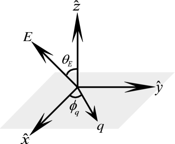
Figure 1: (Color online). Schematic sketch of the 2D monolayer dipolar system in momentum space. The polarization direction of dipolar molecules is controlled by the external electric field $\vec{E}$, which is in the $xz$ plane.

The leading order irreducible polarizability is given by the bare bubble diagrams Mahan (2000) and for the spinless fermions we have

$$\Pi({\bf q},\omega)=\int\dfrac{d^{2}k}{(2\pi)^{2}}\dfrac{n_{F}(\xi_{\bf k})-n_{F}(\xi_{\bf k+q})}{\omega+\xi_{\bf k}-\xi_{\bf k+q}+i\eta}$$ (4)

where $\xi_{\bf k}=\hbar^{2}k^{2}/2m$ is the energy of single particle and $n_{F}$ is the Fermi distribution function. At zero temperature, the polarizability was calculated by SternStern (1967) and the exact expressions, written in terms of dimensionless parameters $x=q/2k_{F}$ ($k_{F}$ is the Fermi wave vector) and $\delta=\omega/4E_{F}$ ($E_{F}$ is the Fermi energy), is given by Galitski and Das Sarma (2004):

$$\begin{array}[]{l l l }\text{Re}\Pi(x,\delta)=\dfrac{m}{2\pi x}\Big{[}\text{sgn}(x-\frac{\delta}{x})\sqrt{(x-\frac{\delta}{x})^{2}-1}\\ \ \ \ \ \ \ \ \ \ \ \ \ \ \ \ \ \ \ \ \ \ +\sqrt{(x+\frac{\delta}{x})^{2}-1}-1\Big{]}\\ \\ \text{Im}\Pi(x,\delta)=\dfrac{m}{4\pi x}\Big{[}\sqrt{1-(x+\frac{\delta}{x})^{2}}-\sqrt{1-(x-\frac{\delta}{x})^{2}}\Big{]}\end{array}$$ (5)

where $\text{Re}\Pi(x,\delta)$ and $\text{Im}\Pi(x,\delta)$ are the real part and the imaginary part of the polarizability, respectively.

We could further introduce some dimensionless parameters which we will use in the following discussions: $s=\frac{md^{2}}{2\hbar^{2}c}$ and $r=2d^{2}k_{F}m/\hbar^{2}$ which describes the strength of dipolar interaction. For example, experimental parameters of fermionic ⁴⁰K⁸⁷Rb ($m=127$ amu,$d=0.57$ Debye, $n=10^{8}$cm^-2), we have $c=10$ nm ($ck_{F}\sim 0.03\ll 1$), $s\simeq 31$ ($s\gg 1$) and $r=4.4$. We use these parameters in the numerical calculation.

For a single layer fermionic dipolar system, the collective modes can be found by looking for the zeros of the dynamical dielectric function, i.e.,

$$\epsilon(q,\omega)=1-V(q)\Pi(q,\omega)=0.$$ (6)

First, we consider the leading order wave vector dependence of the collective mode. In the long wavelength limit ($\omega\gg qv_{F}$, where $v_{F}=k_{F}/m$ is the Fermi velocity), the 2D polarizability becomes

$$\Pi(q,\omega)=\alpha\frac{q^{2}}{\omega^{2}}+O(\frac{q^{4}}{\omega^{4}}),$$ (7)

where $\alpha={n}/{m}$, ($n$ is the 2D density of the dipolar molecules and is related to the Fermi wave vector $k_{F}$ as $k_{F}=\sqrt{4\pi n}$). Then, we have the collective mode in the long wave length ($q\rightarrow 0$)

$$\omega(q)\simeq q\sqrt{(2\pi d^{2}P_{2}(\cos\theta_{E})(\frac{1}{c}-q)+\pi d^{2}q\sin^{2}\theta_{E}\cos 2\phi_{q})\dfrac{n}{m}}$$ (8)

As $\theta_{E}$ varies from 0 to $\frac{\pi}{2}$ by changing the direction of external field, the dipolar interaction changes from an isotropic repulsive to an attractive one at large value of $\theta_{E}$. The plasmon mode given in Eq. (8) depends on both the direction of the external field and the direction of the 2D wave vector. Since the 2D dipolar interaction in the wave vector space has both s-wave and d-wave symmetry as shown in Eq. (3), we only need to consider the case with $\phi_{q}$ in the range $[0,\frac{\pi}{2}]$. As special cases we investigate the plasmon modes along the $x$-axis and $y$-axis, which corresponds to $\phi_{q}=0$ and $\phi_{q}=\frac{\pi}{2}$. For $\phi_{q}=0$, we have the plasmon mode at long wave length limit from Eq. (8):

$$\omega\simeq q\sqrt{(2\pi d^{2}P_{2}(\cos\theta_{E})(\frac{1}{c}-q)+\pi d^{2}q\sin^{2}\theta_{E})\dfrac{n}{m}}.$$ (9)

We find from the above formula that when the electric field is perpendicular to the $xy$ plane (i.e. $\theta_{E}=0$), the plasmon mode becomes

$$\omega(q\rightarrow 0)\simeq q\sqrt{\dfrac{2\pi d^{2}n}{c\ m}}.$$ (10)

Using $k_{F}=\sqrt{4\pi n}$ and $s=\dfrac{md^{2}}{2\hbar^{2}c}$ we have

$$\omega(q\rightarrow 0)\simeq v_{F}\sqrt{s}q.$$ (11)

Since $s\gg 1$, the plasmon mode shown in Eq. 10 satisfies the consistency criterion $\omega\gg qv_{F}$, which has been used to get the 2D polarizability up to the leading order in wave vector. Note that for $\omega>v_{F}q$ the mode lies above the single particle excitation (SPE) regime (or particle-hole continuum) and prevents its direct decay through coupling to particle-hole continuum. The SPE region is defined by the nonzero value of the imaginary part of the total dielectric function, Im$[\epsilon(q,\omega)]\neq 0$, which gives rise to the damping of a plasmon mode by emitting a particle-hole pair excitationHwang and Das Sarma (2009).

When the direction of electric field satisfies $3\cos^{2}\bar{\theta}=1$ (or $\bar{\theta}\simeq 55^{\circ}$), the short distance cut-off disappears and the plasmon dispersion relation becomes

$$\omega\simeq q^{\frac{3}{2}}\sqrt{\dfrac{2\pi d^{2}n}{3m}}=\sqrt{\dfrac{rq}{12k_{F}}}v_{F}q.$$ (12)

We see that the undamped plasmon mode in Eq. (12) exists only for $q>q_{c}=12k_{F}/r$. For $q<q_{c}$ the mode enters into the single particle excitation region and it is damped by producing particle-hole pair. As the external electric field is further tilted leading to $3\cos^{2}\theta_{E}<1$ the solution for $\omega$ satisfying Eq. (6) is purely imaginary, and there is no well-defined collective mode. Thus, along $x$ axis, the direction of the external electric field must be smaller than the critical direction $\theta_{c}$ in order to exist an undamped plasmon mode.

Now we consider the collective mode along the $y$-axis (i.e. $\phi_{q}=\frac{\pi}{2}$). The plasmon mode for this case derived from Eq. (8) is given by

$$\omega(q)\simeq q\sqrt{(2\pi d^{2}P_{2}(\cos\theta_{E})(\frac{1}{c}-q)-\pi d^{2}q\sin^{2}\theta_{E})\dfrac{n}{m}}$$ (13)

For an electric field being perpendicular to the single layer plane $\theta_{E}=0$, the plasmon mode of the system is isotropic and it is the same as given in Eq. (11). For $3\cos^{2}\theta_{E}=1$, there is an undamped mode at $\omega\ll qv_{F}$ and $q>2k_{F}$ because Lindhard function becomes negative and the dipolar interaction $V_{2D}(q)$ is also negative along $y$-axis for $3\cos^{2}\theta_{E}=1$. To get this unusual mode we expand the 2D polarizability for $\omega\ll qv_{F}$ as

$$\Pi(x,\delta)=\dfrac{m}{2\pi}\Big{[}\frac{\sqrt{-1+x^{2}}}{x}-1-\frac{\delta^{2}}{2\left(x^{3}\left(-1+x^{2}\right)^{3/2}\right)}\Big{]}.$$ (14)

Using this large $q$ behavior of the polarizability and Eq. (6) we have the undamped low energy collective mode for $\phi_{q}=\frac{\pi}{2}$ and $\theta_{E}=\bar{\theta}$, which is consistent with the numerical result shown in the left panel of Fig. 2.

$$\omega=\frac{v_{F}q}{2\sqrt{2}\sqrt{r}}\left(-4+\frac{q^{2}}{k_{F}^{2}}\right)^{3/4}\sqrt{6-\frac{qr}{k_{F}}+\sqrt{-4+\frac{q^{2}}{k_{F}^{2}}}r}.$$ (15)

The low energy mode at large wave vectors does not exist in the usual two dimensional electron system (2DES) since the interaction of 2DES is isotropic and positive. This mode is unique for a fermionic dipolar system. Compared with the 2D fermionic dipolar system, the long wave-length plasma frequency for the extensively studied 2DES is written asDas Sarma and Hwang (2009)

$$\omega_{2}(q\rightarrow 0)=\sqrt{\dfrac{2\pi ne^{2}}{\kappa m}}q^{1/2}+O(q^{3/2})$$ (16)

where $n$ and $m$ are the charge carrier density and the effective mass of the charge carriers in the 2DES, respectively. The plasma frequency for the 2DES is isotropic and proportional to $\sqrt{q}$, while the plasma frequency of the 2D dipolar system is characterized by Eq. 8, which is anisotropic and has two different dispersions at long wave-length limit.

In Fig. 2, we show numerically calculated collective mode dispersions of single layer dipolar system for three different external electric field directions $\theta_{E}$. The calculated numerical results agree well with the analytical results discussed above. We choose $\theta_{E}=53^{\circ}$ (it can be any angle close to the critical value $\bar{\theta}$) to investigate the behavior of the collective mode near to the critical angle $\theta_{E}=\bar{\theta}$.

When the 2D wave vector is along the $x$-axis ($\phi_{q}=0$), the slope of plasmon dispersion decreases as the electric field direction increases. In particular, for $\theta_{E}>\bar{\theta}\approx 55^{\circ}$, the plasmon mode enters into the SPE region and it is overdamped by producing particle-hole pair. On the other hand, when the 2D wave vector along the $y$-axis ($\phi_{q}=\frac{\pi}{2}$), the plasmon mode has similar feature as the case for $\phi_{q}=0$ and for smaller angle of $\theta_{E}$. When $\theta_{E}$ approaches to the critical value $\bar{\theta}$ (i.e., $\bar{\theta}\simeq 55^{\circ}$), the long-wave length plasmon mode approaches to the upper boundary of the SPE region (i.e., $\omega={q^{2}}/{2m}+v_{F}q$). The main difference between $\phi_{q}=0$ and $\phi_{q}=\pi/2$ cases is that there is a short-wave length plasmon mode for the latter case even at $3\cos^{2}\theta_{E}\leq 1$. This plasmon mode for $\phi_{q}=\pi/2$ appears below the lower boundary of the SPE region (i.e., $\omega={q^{2}}/{2m}-v_{F}q$), where both the dipolar interaction and the Lindhard function are negative.

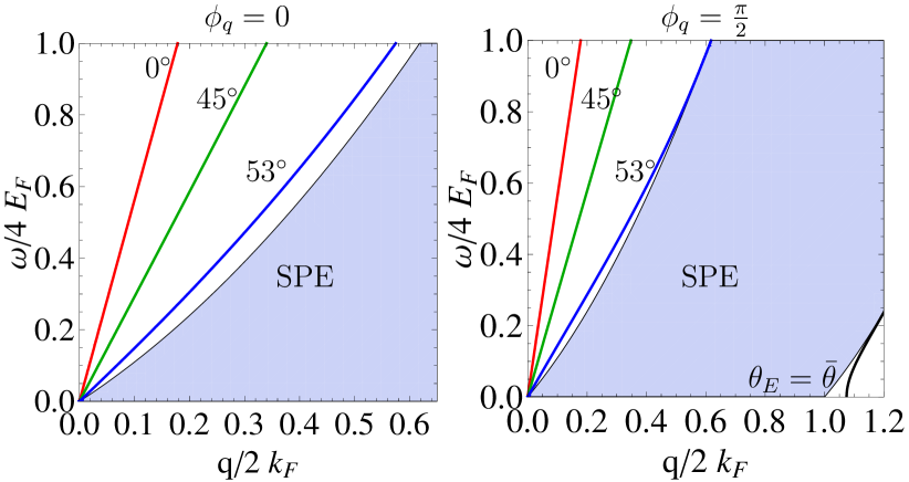
Figure 2: (Color online). Calculated plasmon mode dispersions of single layer dipolar system for different external electric field direction $\theta_{E}$. The shadowed region indicate the single-particle excitation (SPE) region. The interaction parameter $r=4.4$ and $s=31$ are used in this calculation. The mode dispersions (a) for $\phi_{q}=0$ and (b) for $\phi_{q}=\dfrac{\pi}{2}$ are shown.

III Plasmon mode in Bilayer dipolar system

For a bilayer system, which is parallel to the $xy$ plane and is separated by a distance $a$, we need to consider the generalized dielectric tensor $\epsilon$ Das Sarma and Madhukar (1981) in order to find the collective modes. Within the RPA the $lm$ component of the dielectric tensor is given by

$$\epsilon_{lm}(q,\omega)=\delta_{lm}-V_{lm}(q)\Pi_{m}(q,\omega),$$ (17)

where $l,m=1$ or 2 with 1,2 denoting the index of two different layers. Then the plasmon modes are given by the zeros of the two-component determinantal equation, i.e.,

$$\begin{array}[]{l c c c c c c}\epsilon(q,\omega)=[1-V_{11}(q)\Pi_{1}(q,\omega)][1-V_{22}(q)\Pi_{2}(q,\omega)]\\ \\ \ \ \ \ \ \ \ \ -V_{12}(q)V_{21}(q)\Pi_{1}(q,\omega)\Pi_{2}(q,\omega)=0,\end{array}$$ (21)

where $\Pi_{l}$ is the polarizability of layer $l$ and is given by Eq. (4), and $V_{ll}$ and $V_{lm}$ are, respectively, the intralayer and interlayer dipolar interaction. The intralayer dipolar interaction is the same as given in Eq. (3)

$$\begin{array}[]{l c c c c c c}V_{11}(q)=V_{22}(q)=2\pi d^{2}P_{2}(\cos\theta_{E})(\dfrac{1}{c}-q)\\ \ \ \ \ \ \ \ \ \ \ \ \ +\pi d^{2}\sin^{2}\theta_{E}\cos 2\phi_{q}q\\ \ \ \ \ \ \ \ \ =\pi d^{2}(3\cos^{2}\theta_{E}-1)\dfrac{1}{c}\\ \ \ \ \ \ \ \ \ \ \ \ \ +2d^{2}q\pi(\sin^{2}\theta_{E}\cos^{2}\phi_{q}-\cos^{2}\theta_{E}).\end{array}$$ (26)

For the 2D bilayer dipolar system the interlayer interaction $V_{12}$ is given in real space

$$V_{12}(\vec{r})=\frac{d^{2}}{(r^{2}+a^{2})^{\frac{3}{2}}}\left[1-\frac{3(r\cos\phi\sin\theta_{E}+h\cos\theta_{E})^{2}}{r^{2}+h^{2}}\right],$$ (27)

where $\theta_{E}$ is the polar angle of an external electric field which is applied in the $xz$ plane and $\phi_{q}$ is the azimuthal angle measuring from $x$-axis. Note that $V_{12}(-\vec{r})\neq V_{12}(\vec{r})$ if the electric field is not perpendicular to the $xy$ plane, which gives rise to the imaginary component for the interlayer interaction in the wave vector space. The detailed calculation for $V_{12}(q)$ is given in Appendix. A and we express the following explicit form of the interlayer interaction in momentum space as:

$$\begin{array}[]{l c c c c c c}V_{12}(q)=2d^{2}q\pi e^{-aq}(\sin^{2}\theta_{E}\cos^{2}\phi_{q}-\cos^{2}\theta_{E}\\ \\ \ \ \ \ \ \ \ \ \ \ \ \ -\sin 2\theta_{E}\cos\phi_{q}\ i)\end{array}$$ (31)

and

$$\begin{array}[]{l c c c c c c}V_{21}(q)=2d^{2}q\pi e^{-aq}(\sin^{2}\theta_{E}\cos^{2}\phi_{q}-\cos^{2}\theta_{E}\\ \\ \ \ \ \ \ \ \ \ \ \ \ \ +\sin 2\theta_{E}\cos\phi_{q}\ i)\end{array}$$ (35)

We note that both the interlayer and intralayer interaction depends on both the direction of momentum $q$ and the direction of an electric field $\vec{E}$. In addition, there is a short distance cutoff in interlayer interaction, Eq. (26), but not in the intralayer interaction. The interlayer distance $a$ should be larger than the short distance cutoff $c$ beyond which the interaction between two dipole molecules can be described by the dipolar interaction. Typically in the cold atomic system, the interlayer distance $a=500$nm and we use $c=10$nm as the short distance cut-off for the intralayer interaction as done in the single layer dipolar system. Alternatively, we can assume that the two layers separated by a distance $a$ are strongly confined in the $z$ direction with Gaussian distribution in the $z$ direction, $n(z)\propto e^{{-(z\pm a/2)^{2}}/{2w^{2}}}$. In the wave vector space we have $n(k_{z})=e^{-{w^{2}k_{z}^{2}}\pm i{d}/{2}k_{z}}$. Then, we get the same interlayer interaction when we integrate out the $k_{z}$ part of the 3D dipolar interaction. The numerical factor before $1/w$ is suppressed by $e^{-\frac{a^{2}}{2w^{2}}}$ of Eq. (1) in Ref. [Kestner and Das Sarma, 2010], which means that the term with $1/w$ can be neglected as long as $a/w\gg 1$. We numerically checked that the interlayer interaction with Gaussian distribution agree well with Eq. (31) as long as $a/c>5$, which is the case we consider in our work.

III.1 Long wavelength plasmon mode in bilayer dipolar system

In this subsection, we derive the analytical results of plasmon mode in the long wave length limit. We first consider the leading order wave vector dependence of the plasmon mode in the bilayer dipolar gas. At zero temperature, the two dimensional non-interacting polarizability has the following limiting forms in the high frequency regimes (i.e., $\omega\gg qv_{F}$)Das Sarma and Madhukar (1981):

$$\Pi_{i}(q,\omega)=\alpha_{i}\frac{q^{2}}{\omega^{2}}+O(\frac{q^{4}}{\omega^{4}})$$ (36)

where $i=1$ or 2 with 1,2 denoting the two different layers, and $\alpha_{i}={n_{i}}/{m}$, $n_{i}$ is the dipolar molecule density of the $i$th layer. Then, combining Eq. (21,26) and Eqs. (31)-(36), we obtain the long-wavelength plasmon modes of the bilayer dipolar system:

$$\begin{array}[]{l l }\omega^{2}_{\pm}\simeq\dfrac{q^{2}}{2}\big{(}\alpha_{1}V_{11}+\alpha_{2}V_{22}\\ \\ \ \ \ \ \ \pm\sqrt{(\alpha_{1}V_{11}-\alpha_{2}V_{22})^{2}+4\alpha_{1}\alpha_{2}V_{12}V_{21}}\big{)},\end{array}$$ (40)

where $\omega_{+}$ ($\omega_{-}$) indicates the optical (acoustic) plasmon mode where the density fluctuations in each layer oscillate in-phase (optical) and out-of-phase (acoustic) relative to each other, respectively. Eq. 40 is also valid for the ordinary bilayer 2DES, while the interlayer and intralayer interaction is written as:

$$\begin{array}[]{l c c c c c c}V_{11}(q)=V_{22}(q)=\dfrac{2\pi e^{2}}{q}\\ \\ V_{12}(q)=V_{21}(q)=\dfrac{2\pi e^{2}}{q}e^{-aq}.\end{array}$$ (44)

which are both isotropic. In the strong coupling ($qa\ll 1$) and long wave-length limit, we have the following two plasma frequencies for the 2DES:

$$\begin{array}[]{l c c c c c c}\omega_{+}\simeq\sqrt{\dfrac{2\pi e^{2}(n_{1}+n_{2})}{\kappa m}}q^{1/2}\\ \\ \omega_{-}\simeq\sqrt{\dfrac{2\pi e^{2}n_{1}n_{2}}{\kappa m(n_{1}+n_{2})}}q\end{array}$$ (48)

While in the weak coupling ($qa\gg 1$) and long wave-length limit , the modes are simply the respective two-dimensional plasma frequencies of the two componentsDas Sarma and Madhukar (1981):

$$\begin{array}[]{l c c c c c c}\omega_{+}\simeq\sqrt{\dfrac{2\pi n_{1}e^{2}}{\kappa m}}q^{1/2}\\ \\ \omega_{-}\simeq\sqrt{\dfrac{2\pi n_{2}e^{2}}{\kappa m}}q^{1/2}\end{array}$$ (52)

Now we investigate the plasmon modes of this bilayer dipolar system in two regimes: the strong coupling limit ($qa\ll 1$) and the weak coupling limit ($qa\gg 1$).

III.1.1 Strong coupling limit $qa\ll 1$

When the external electric field is perpendicular to the bilayer plane, i.e., $\theta_{E}=0$, the interlayer and intralayer interaction become for $qa\ll 1$

$$\begin{array}[]{l c c c c c c}V_{11}(q)=V_{22}(q)=2\pi d^{2}(\dfrac{1}{c}-q)\\ \\ V_{12}(q)=V_{21}(q)=-2\pi d^{2}qe^{-aq}.\end{array}$$ (56)

Then the long wavelength plasmon modes become

$$\omega^{2}_{\pm}\simeq\dfrac{q^{2}\pi d^{2}}{c}\left[\alpha_{1}+\alpha_{2}\pm\sqrt{(\alpha_{1}-\alpha_{2})^{2}+4q^{2}c^{2}\alpha_{1}\alpha_{2}}\right].$$ (57)

Because the short distance cut-off in the intralayer dipolar interaction is set to satisfy $k_{F_{1,2}}\ll\frac{1}{c}$ and $r_{1,2}=2md^{2}k_{F_{1,2}}$, it is clear to see that the above two plasmon modes also satisfy the self-consistent criterion $\omega\gg qv_{F}$. These two modes lies outside of the SPE region, which are undamped and stable. Since the external electric field is perpendicular to the $xy$ plane, the bilayer dipolar system is purely isotropic, which gives rise to the plasmon mode to be independent of the wave vector direction, $\phi_{q}$.

For $\theta_{E}=\bar{\theta}\approx 55^{\circ}$, the system is purely anisotropic and the plasmon modes are given by

$$\begin{array}[]{l l l}\omega^{2}_{\pm}\simeq\dfrac{d^{2}\pi q^{3}}{3}\Big{[}(\alpha_{1}+\alpha_{2})\cos 2\phi_{q}\\ \\ \ \ \ \ \ \pm\sqrt{(\alpha_{1}-\alpha_{2})^{2}\cos^{2}2\phi_{q}+4\alpha_{1}\alpha_{2}(2+\cos 2\phi_{q})^{2}}\Big{]}.\end{array}$$ (61)

When the 2D wave vector is along the $x$-axis (i.e., $\phi_{q}=0$), the $\omega_{-}$ plasmon mode is overdamped since $\omega_{-}$ becomes pure imaginary. But, the in-phase mode is well defined as long as $r\gg 1$ (in order to satisfy the self-consistent criterion $\omega\gg qv_{F}$) and the plasmon mode is given by

$$\begin{array}[]{l l l}\omega^{2}_{+}\simeq\dfrac{d^{2}\pi q^{3}}{3}\Big{[}(\alpha_{1}+\alpha_{2})+\sqrt{(\alpha_{1}+\alpha_{2})^{2}+32\alpha_{1}\alpha_{2}}\Big{]}.\end{array}$$ (63)

However, along the $y$-axis ($\phi_{q}=\pi/2$), both $\omega_{-}$ and $\omega_{+}$ plasmon modes are pure imaginary, and there are no well-defined collective mode in the long wavelength limit.

III.1.2 weak coupling limit $qa\gg 1$

In weak coupling limit $e^{-aq}\approx 0$ and the interlayer interaction between two layers is much weaker than the intralayer interaction, which give rise to the two independent plasmon modes of each layer. Thus we have uncoupled plasmon modes as

$$\begin{array}[]{l c c c c c c}\omega^{2}_{+}=q^{2}\alpha_{1}(2\pi d^{2}P_{2}(\cos\theta_{0})(\frac{1}{c}-q)+\pi d^{2}\sin^{2}\theta_{0}q)\\ \\ \omega^{2}_{-}=q^{2}\alpha_{2}(2\pi d^{2}P_{2}(\cos\theta_{0})(\frac{1}{c}-q)+\pi d^{2}\sin^{2}\theta_{0}q).\end{array}$$ (67)

The detailed discussion about the existence of plasmon modes in this weak coupling limit is the same as that for single layer dipolar gas. If the two layers have the same density and mass, $\omega^{2}_{+}=\omega^{2}_{-}$, i.e., two plasmon modes have the same dispersion relation.

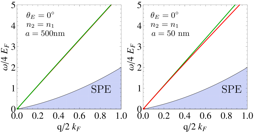
Figure 3: (Color online). Calculated plasmon mode dispersions of bilayer dipolar system for two different interlayer distances (a) $a=0.5\mu$m and (b) $a=50$ nm at $\theta_{E}=0^{\circ}$. We use $n_{1}=n_{2}=10^{8}$cm^-2 and $r=4.4$ and $s=31$ in this calculation. The shadowed region indicate the single-particle excitation (SPE) region.

III.2 Numerical results of plasmon modes in bilayer dipolar system

In this subsection, we show our numerical results of plasmon modes for the bilayer dipolar system with typical parameters of ⁴⁰K⁸⁷Rb. In Fig. 3 we show the calculated plasmon dispersions for an external electric field perpendicular to $x$-$y$ plane ($\theta_{E}=0$) with equal densities of $n_{1}=n_{2}=10^{8}$cm^-2. When the separation of two layers are much larger than the inverse of the Fermi wave vector (i.e. weak coupling limit), the interlayer interaction is negligible and the bilayer dipolar system behave like two independent single layers. Thus, two plasmon modes are almost degenerated and there is only one plasmon mode showed up in the left panel of Fig.3. When the two layers are getting closer, the interlayer interaction become stronger. As a consequence, the density fluctuation in each layer is coupled and the degenerated plasmon mode is split into two plasmon modes, especially at large wave vectors, as shown in the right panel of Fig.3.

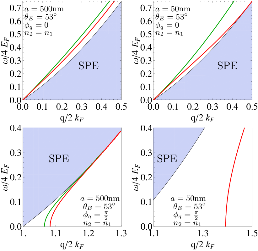
Figure 4: (Color online). Calculated plasmon mode dispersions of double layer dipolar system for two different interlayer distance and $\phi_{q}$ at $\theta_{E}=53^{\circ}$ with $n_{1}=n_{2}=10^{8}$cm^-2. The shadowed region indicate the single-particle excitation (SPE) region. The solid lines are solutions for $\epsilon(q,\omega)=0$ for $r=4.4$ and $s=31$.

In Fig. 4 we show the calculated plasmon dispersions for $\theta_{E}=53^{\circ}$, (i.e., the direction of an external electric field is close to the critical angle of $\theta_{E}=55^{\circ}$). The plasmon dispersions are calculated with equal densities of $n_{1}=n_{2}=10^{8}$cm^-2 for two different interlayer distance ($a=500$nm and 50nm) and two different directions of the wave vector ($\phi_{q}=0$ and $\pi/2$) because of the anisotropic properties of the interlayer interaction. (Note that for $\theta_{E}=0$ the plasmon modes are isotropic and independent of $\phi_{q}$). Since $\theta_{E}$ is close to the critical angle the plasmon modes approach to the upper boundary of the electron-hole continuum. For $\phi_{q}=0$ (i.e. the 2D wave vector is along $x$-axis) both in-phase and out of phase plasmon modes are located above the SPE region and they are undamped. As long as $\theta_{E}\geq\bar{\theta}_{E}$ we find two undamped modes even though the two modes are almost degenerate for weak coupling limit. When the layer separation is small (i.e., strong coupling limits), the out-of-phase mode (lower energy mode) gets closer to the SPE region. For $\theta_{E}\geq\bar{\theta}_{E}$ the out-of-phase mode enters into the SPE and is overdamped. Thus, there is only one undamped mode for $\theta_{E}\geq\bar{\theta}_{E}$. For $\phi_{q}=\pi/2$ both modes have similar feathers as that for $\phi_{q}=0$ but they are very close to the upper boundary of SPE region. When the $\theta_{E}$ is greater than the critical angle we find no plasmon modes above the upper boundary of SPE region (i.e., $\omega=\dfrac{q^{2}}{2m}+v_{F}q$). But there are plasmon modes appearing below the lower boundary of SPE region (i.e., $\omega={q^{2}}/{2m}-v_{F}q$) for $\phi_{q}=\pi/2$ (the lower panel of Fig. 4). As the interlayer coupling gets stronger, the in-phase mode with higher frequency is pushed into the SPE region and only the out-of-phase mode with lower frequency survived.

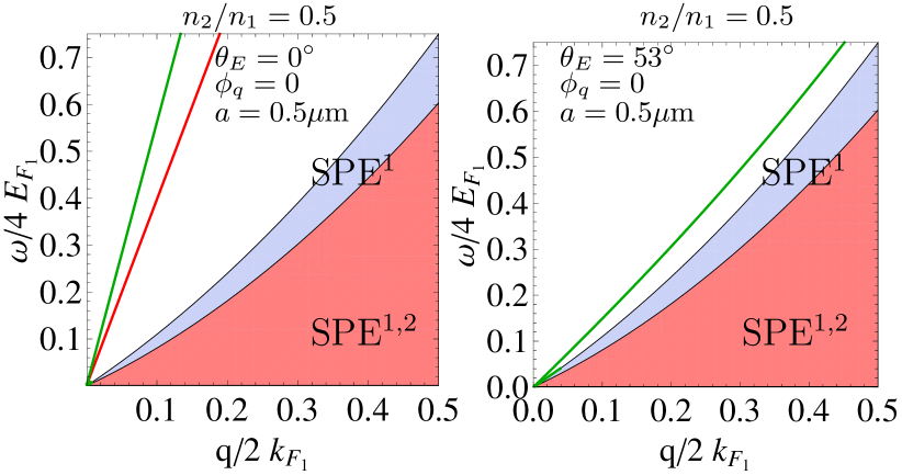
Figure 5: (Color online). Calculated plasmon mode dispersions of double layer dipolar system for two different $\theta_{E}$ at $\phi_{q}=0$ with $n_{1}=10^{8}$cm^-2 ($k_{F}=\sqrt{4\pi n_{1}}$), $n_{2}/n_{1}=0.5$ and interlayer distance $a=0.5\mu$m. The shadowed region indicate the single-particle excitation (SPE) region. The solid lines are solutions for $\epsilon(q,\omega)=0$ for $r=4.4$ and $s=31$. The left panel is for the electric field perpendicular to the $xy$ plane $\theta_{E}=0^{\circ}$, while the right panel is for the electric field titled at $\theta_{E}=53^{\circ}$.

In Fig. 5, we calculated plasmon mode dispersions of bilayer dipolar system with different densities ($n_{2}/n_{1}=0.5$) for two different $\theta_{E}$ at $\phi_{q}=0$. Fig. 5(a) presents the plasmon modes for the isotropic interaction, i.e., the external electric field is perpendicular to the $xy$ plane ($\theta_{E}=0^{\circ}$). For a large interlayer distance ($a=0.5\mu$m), the coupling between the two layers is very weak and they behave like two independent layers as shown in Eq. (67). From Eq. (67), we know that, for $\theta_{E}=0$ and weak coupling limit, both plasmon modes have linear dispersion relation and the slope of the plasmon modes is proportional to their densities. Thus, two separated plasmon modes are undamped. Fig. 5(b) shows the plasmon dispersion of the anisotropic bilayer dipolar system for $\theta_{E}=53^{\circ}$, $\phi_{q}=0$ and $a=0.5\mu$m. There is only one undamped mode $\omega_{+}$ because $\omega_{-}$ lies inside the SPE region.

In Figs. 6 and 7 we show the calculated loss function (i.e., -Im$[\epsilon(k_{F},\omega)^{-1}]$) of the bilayer dipolar system for a fixed wave vector ($q=k_{F}$). The loss function is related to the dynamical structure factor $S(q,\omega)$ by $S(q,\omega)\propto$-Im$[\epsilon(k_{F},\omega)^{-1}]$ and the dynamical structure factor gives the direct measure of the spectral strength of the various elementary excitationsGiuliani and Vignale (2005); Hwang and Das Sarma (2009). We plot the loss functions in $(\omega,\phi_{q})$ space to describe the angular dependence of the plasmon modes. The loss function is an experimental observable which can be measured with Raman-scattering spectroscopies. The plasmon modes exist when both real and imaginary part of the dielectric function equal zero (i.e., Re$[\epsilon(q,\omega)]=0$ and Im$[\epsilon(q,\omega)]=0$), which leads the imaginary part of the inverse dielectric function -Im$[\epsilon(k_{F},\omega)^{-1}]$ to be a $\delta$-function indicating an undamped plasmon modes. On the other hand, the broadened peak in the loss function gives the damped plasmon modes. The damping in the plasmon mode is induced by particle-hole pair creation because we neglect any disorder effects in this calculation.

In Fig. 6(a) we show the result when the applied electric field is perpendicular to the plane. In this case both interlayer and intralayer interaction are isotropic. The solid circle gives the undamped plasmon modes, at which the loss function becomes singular. Since two plasmon modes are degenerate and they are independent of the wave vector direction $\phi_{q}$, the plasmon modes appear as one solid circle in the ($\omega,\phi_{q}$) space. For $\theta_{E}=53^{\circ}$, the two plasmon modes can also clearly be seen in Fig.6(b). For $\theta_{E}=53^{\circ}$, both intralayer and interlayer interaction are anisotropic, so that the plasmon modes appear as ellipses in the ($\omega,\phi_{q}$) space and they become much closer along the $y$-axis.

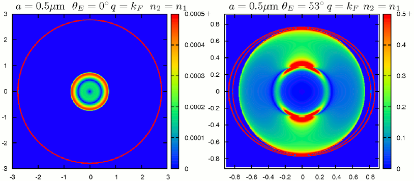
Figure 6: (Color online). The density plots of the absolute value of the loss function -Im$[\epsilon(k_{F},\omega)^{-1}]$ of bilayer dipolar system with same densities in ($\omega,\phi_{q}$) polar coordinate space for fixed density $n_{1}=n_{2}=10^{8}$cm^-2, $r=4.4$, $s=31$, $a=500$nm and $\theta_{E}=0^{\circ}$(left) and $\theta_{E}=53^{\circ}$(right).

In Fig. 7, we present the density plots of the loss function -Im$[\epsilon(k_{F},\omega)^{-1}]$ of bilayer dipolar system for $\theta_{E}=\bar{\theta}$, where the short distance cut-off disappears from the intralayer interaction and the bilayer system becomes totally anisotropic. In Fig. 7 the plasmon modes are shown for interlayer distance (a) $a=0.5\mu$m (strong coupling limit) and (b) $a=50$nm (weak coupling limit). There is no $\delta$-function like peak in the loss function for $q=k_{F}$ in both cases, which correspond to damped plasmon modes.

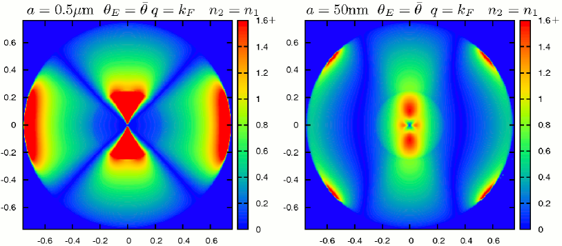
Figure 7: (Color online). The density plots of the absolute value of the loss function -Im$[\epsilon(k_{F},\omega)^{-1}]$ of bilayer dipolar system with same densities in ($\omega,\phi_{q}$) polar coordinate space for fixed density $n_{1}=n_{2}=10^{8}$cm^-2, $r=4.4$, $s=31$, $\theta_{E}=\bar{\theta}$ and $h=500$nm(left) and $a=50$nm(right).

IV Plasmon mode in dipolar superlattice

In this section, we discuss the plasmon modes of a superlattice system which consist of the infinite number of parallel and equally separated two dimensional dipolar system. Due to the long range behavior of the dipolar interaction, it is necessary to couple all the layers, which changes the dielectric function in Eq. (6) to an infinite matrix equationDas Sarma and Hwang (2009):

$$|\delta_{l,l^{\prime}}-V_{l,l^{\prime}}(q)\Pi_{l^{\prime}}(q,\omega)|=0$$ (68)

where $l$ (or $l^{\prime}$)$=0,\pm 1,\pm 2$, …, are the indices of the layers and each layer is placed parallel to the $xy$ plane with the position $z=la$ in the $z$ direction. $V_{l,l^{\prime}}(q)$ is the dipolar interaction between the $l$th and the $l^{\prime}$th layer, which can be written as

$$\begin{array}[]{l l l l l l }l=l^{\prime}:\\ V_{ll}=V_{0}(q)=\pi d^{2}(3\cos^{2}\theta_{E}-1)\dfrac{1}{c}\\ \ \ \ \ \ \ \ \ \ \ \ \ +2d^{2}q\pi(\sin^{2}\theta_{E}\cos^{2}\phi_{q}-\cos^{2}\theta_{E});\\ l\neq l^{\prime}:\\ V_{ll^{\prime}}(q)=2d^{2}q\pi e^{-aq|l-l^{\prime}|}(\sin^{2}\theta_{E}\cos^{2}\phi_{q}-\cos^{2}\theta_{E}\\ \ \ \ \ \ \ \ \ \ \ \ \ -i\text{sgn}(l-l^{\prime})\sin 2\theta_{E}\cos\phi_{q}),\end{array}$$ (69)

where $a$ is the superlattice period (i.e., the separation between adjacent layers in the $z$ direction), $\text{sgn}(l-l^{\prime})$ equals $1(l>l^{\prime})$ or $-1(l<l^{\prime})$, and $\Pi_{l^{\prime}}(q,\omega)=\Pi(q,\omega)$ is the irreducible polarizability of each 2D dipolar system given in Eq.4. The difference between intralayer and interlayer interaction in calculating the dipolar system is that the intralayer interaction in momentum space has the short distance cut-off $c$, while the interlayer interaction does not depending on this short distance cut-off.

The plasmon modes of the infinite periodic system can be calculated from the self-consistent field method described in Ref. [Das Sarma and Quinn, 1982]. Since the superlattice is perfectly periodic in the $z$ direction with periodicity $a$, we assume the following ansatz $n_{l}(q,\omega)=n_{0}(q,\omega)e^{ik_{z}la}$, where $a$ is the interlayer distance and $l$ is the layer index. The $k_{z}$ introduced in the above ansatz labels the induced density fluctuation in the infinite periodic system, which is restricted in the first Brillouin zone of the superlattice, i.e., $0\leq k_{z}\leq\frac{2\pi}{a}$. Then the plasmon modes for the dipolar superlattice system are given by the roots of following equation

$$1-\Pi(q,\omega)V_{0}(q)-\Pi(q,\omega)\sum_{l^{\prime}(l\neq l^{\prime})}V_{ll^{\prime}}(q)e^{-ik_{z}(l-l^{\prime})a}=0$$ (70)

where $V_{0}(q)$ is the intralayer interaction in momentum space while $V_{l-l^{\prime}}(q)$ is the interlayer interaction. With the help of formula given in Appendix. B, Eq. (70) can be explicitly written as:

$$1-\Pi(q,\omega)V_{0}(q)-\Pi(q,\omega)2d^{2}q\pi\big{[}(\sin^{2}\theta_{E}\cos^{2}\phi_{q}-\cos^{2}\theta_{E})S_{1}(q,k_{z})-\sin 2\theta_{E}\cos\phi_{q}S_{2}(q,k_{z})\big{]}=0,$$ (71)

where

$$S_{1}(q,k_{z})=\dfrac{\cos k_{z}a-\exp{(-aq)}}{\cosh aq-\cos k_{z}a},$$ (72)

and

$$S_{2}(q,k_{z})=\dfrac{\sin k_{z}a}{\cosh aq-\cos k_{z}a}.$$ (73)

We investigate the long wavelength plasmon modes for the strong coupling $qa\gg 1$ and the weak coupling case $qa\ll 1$ analytically in the following two subsections.

IV.1 Strong coupling case $qa\ll 1$

First, we consider the $k_{z}\neq 0$ case. With the asymptotic form of the polarizability $\Pi(q,\omega)\simeq\dfrac{n}{m}\dfrac{q^{2}}{\omega^{2}}$ we can rewrite Eq. (71) for $qa\ll 1$ as

$$1-2\pi d^{2}\dfrac{nq^{2}}{m\omega^{2}}\Big{[}\dfrac{P_{2}(\cos\theta_{E})}{c}+(\sin^{2}\theta_{E}\cos^{2}\phi_{q}-\cos^{2}\theta_{E})\dfrac{aq^{2}}{1-\cos k_{z}a}-q\sin 2\theta_{E}\cos\phi_{q}\dfrac{\sin k_{z}a}{1-\cos k_{z}a}\Big{]}=0.$$ (74)

Then we have the plasmon modes for the superlattice dipolar system in the long length limit

$$\omega^{2}\simeq q^{2}\dfrac{2n\pi d^{2}}{m}\Big{[}\dfrac{P_{2}(\cos\theta_{E})}{c}+(\sin^{2}\theta_{E}\cos^{2}\phi_{q}-\cos^{2}\theta_{E})\dfrac{aq^{2}}{1-\cos k_{z}a}\Big{]}.$$ (75)

The plasmon mode in superlattice system is strongly dependent on the direction of the external electric field $\theta_{E}$ and the wave vector direction $\phi_{q}$ as well as the wave vector $k_{z}$ that labels the density fluctuation. When the electric field is perpendicular to the plane, we find that the plasmon mode has linear dispersion relation $\omega\propto q$. For $\theta_{E}=\bar{\theta}$, in which the interactions are anisotropic, the plasmon mode dispersion becomes

$$\omega\simeq q^{\frac{3}{2}}\sqrt{\dfrac{2n\pi d^{2}}{3m}\big{(}\dfrac{aq\cos 2\phi_{q}}{1-\cos k_{z}a}-2\sqrt{2}\frac{\cos\phi_{q}\sin k_{z}a}{1-\cos k_{z}a}\big{)}}.$$ (76)

In order for this mode to lie above the SPE region, i.e. $\omega>qv_{F}$, it is required to be $r\gg 1$.

For $k_{z}=0$, the long wavelength plasmon mode can be calculated from Eq. (71) to be

$$\omega^{2}\simeq\dfrac{q^{2}2n\pi d^{2}}{m}\Big{[}\dfrac{P_{2}(\cos\theta_{E})}{c}+\dfrac{2(\sin^{2}\theta_{E}\cos^{2}\phi_{q}-\cos^{2}\theta_{E})}{a}\Big{]}.$$ (77)

In particular, the plasmon dispersion for $\theta_{E}=0$ becomes

$$\omega\simeq q\sqrt{\dfrac{2n\pi d^{2}(a-2c)}{mac}}.$$ (78)

From Eq. (78) it is clear that only for $a>2c$ there is well defined plasmon mode with linear dispersion relation. For the total anisotropic case ($\theta_{E}=\bar{\theta}_{E}$), the plasmon mode also has linear dispersion relation which can written as:

$$\omega\simeq q\sqrt{\dfrac{4n\pi d^{2}\cos 2\phi_{q}}{3ma}}.$$ (79)

Thus the plasmon mode only exists for certain angles such that $\cos 2\phi_{q}>0$.

Compared to the dipolar superlattice system, the plasma frequency for the superlattice system with Coulomb interaction can be written asDas Sarma and Hwang (2009):

$$\omega(q\rightarrow 0;k_{z}=0)=\Big{(}\dfrac{4\pi e^{2}n}{a\kappa m}\Big{)}^{1/2}$$ (80)

which has the precise character of the corresponding three dimensional plasmon (with a finite gap) in the long wavelength limit.

IV.2 Weak Coupling case $qa\gg 1$

For the weak coupling ($qa\gg 1$) Eq. (71) becomes

$$1-\Pi(q,\omega)V_{0}(q)=0$$ (81)

for all values of $k_{z}$. Thus the long wavelength plasmon mode of superlattice system becomes the mode of the single layer dipolar system as discussed in Sec.II. Each layer has its own plasmon mode in the weak coupling limits as expected.

V Summary and Conclusions

In summary, we have derived the collective plasmon modes in 2D dipolar Fermi liquids, and also considered spatially separated bilayer and superlattice dipolar systems within the random phase approximation, which is valid for weakly interacting system. We have also calculated the loss function for bilayer fermionic dipolar gas, which could be measured in experiments. The 2D dipolar interaction with both s and d-wave components in the wave vector space leads to several unexpected features in the plasmon modes such as undamped mode if dipole along the $z$-axis and the anisotropic plasmon dispersion relation if the dipole along other direction than the $z$-axis. Our predicted plasmon modes is clearly distinguished from the extensively studied two dimensional electron system.

Future work ought to include higher order corrections to the polarizability and the finite temperature corrections, yet this must await the successful fabrication of quasi two dimensional dilute fermionic dipolar gases. We note that our theory for the collective mode spectra of 2D dipolar Fermi liquids should have considerable relevance for the recently made polar molecular gases Ref. [Ospelkaus et al., 2008; Ni et al., 2008, 2009; Ospelkaus et al., 2010; Griesmaier et al., 2005; Ospelkaus et al., 2009]. At low enough temperatures, $T\ll T_{F}$ where $T_{F}$ is the Fermi temperature of the dipolar system, our theory should in principle describe the laboratory polar molecular fermionic systems, and the excitation spectra of the dipolar system should have clear signatures of the collective mode spectra presented in our work.

Appendix A

Below we provide the detailed calculation of the interlayer dipolar interaction in the wave vector space. In the real space the interlayer dipolar interaction becomes

$$V_{12}(\vec{r})=\frac{d^{2}}{(r^{2}+a^{2})^{\frac{3}{2}}}\left[1-\frac{3(r\cos\phi\sin\theta_{E}+h\cos\theta_{E})^{2}}{r^{2}+h^{2}}\right],$$ (82)

where $\phi_{q}$ is the angle between momentum $q$ and the $x$-axis. We can devide above equation into three different partss depending on the symmetry

$$V^{(a)}_{12}(r)=\frac{d^{2}}{(r^{2}+a^{2})^{\frac{3}{2}}}(1-\frac{3a^{2}\cos^{2}\theta_{0}}{r^{2}+h^{2}}),$$ (83)

$$V^{(b)}_{12}(r)=\frac{d^{2}}{(r^{2}+a^{2})^{\frac{5}{2}}}(3r^{2}\cos^{2}\phi\sin^{2}\theta_{0}),$$ (84)

and

$$V^{(c)}_{12}(r)=\frac{d^{2}}{(r^{2}+a^{2})^{\frac{5}{2}}}(6r\cos\phi\sin\theta_{0}a\cos\theta_{0}),$$ (85)

where $V_{12}(q)=V^{(a)}_{12}(q)-V^{(b)}_{12}(q)-V^{(c)}_{12}(q)$. Then we have

$$\begin{array}[]{l c c c c c c}V^{(a)}_{12}(q)=d^{2}\int_{0}^{\infty}\int_{0}^{2\pi}\dfrac{1-3\frac{a^{2}\cos^{2}\theta_{0}}{a^{2}+r^{2}}}{(a^{2}+r^{2})^{\frac{3}{2}}}\exp(i\vec{q}\cdot\vec{r})rdrd\phi\\ \\ \ \ \ \ \ \ =2q\pi d^{2}e^{-aq}(\dfrac{\sin^{2}\theta_{0}}{aq}-\cos^{2}\theta_{0}),\end{array}$$ (89)

where $J_{0}(x)$ is the Bessel function of the first kind and $\vec{q}\cdot\vec{r}=qr\cos(\phi-\phi_{q})$.

$$\begin{array}[]{l c c c c c c c }V^{(b)}_{12}(q)=d^{2}\int_{0}^{\infty}\int_{0}^{2\pi}\dfrac{3r^{2}\cos^{2}\phi\sin^{2}\theta_{0}}{(a^{2}+r^{2})^{\frac{5}{2}}}\exp(i\vec{q}\cdot\vec{r})rdrd\phi\\ \\ =2d^{2}q\pi e^{-aq}\sin^{2}\theta_{0}(\dfrac{1}{aq}-\cos^{2}\phi_{q}),\end{array}$$ (93)

and

$$\begin{array}[]{l c c c c c c}V^{(c)}_{12}(q)=d^{2}\int_{0}^{\infty}\int_{0}^{2\pi}\dfrac{3r^{2}a\cos\phi\sin 2\theta_{0}}{(a^{2}+r^{2})^{\frac{5}{2}}}\exp(i\vec{q}\cdot\vec{r})drd\phi\\ \\ =2d^{2}q\pi e^{-aq}\sin 2\theta_{0}\cos\phi_{q}\ i\end{array}$$ (97)

which is pure imaginary number. Finally we have the interlayer interaction in momentum space

$$V_{12}(q)=2d^{2}q\pi e^{-aq}(\sin^{2}\theta_{E}\cos^{2}\phi_{q}-\cos^{2}\theta_{E}-\sin 2\theta_{E}\cos\phi_{q}\ i).$$ (98)

We also find $V_{21}(q)$ from $V_{21}(\vec{r})$

$$V_{21}(\vec{r})=\frac{d^{2}}{(r^{2}+a^{2})^{\frac{3}{2}}}\left[1-\frac{3(r\cos\phi\sin\theta_{E}-h\cos\theta_{E})^{2}}{r^{2}+h^{2}}\right]$$ (99)

the interlayer dipolar interaction $V_{21}(q)$ in the wave vector space is given the complex conjugate of $V_{12}(q)$, which can written as:

$$V_{21}(q)=2d^{2}q\pi e^{-aq}(\sin^{2}\theta_{E}\cos^{2}\phi_{q}-\cos^{2}\theta_{E}+\sin 2\theta_{E}\cos\phi_{q}\ i)$$ (100)

Appendix B

Below we provide detailed calculation of two infinite sums in Sec. IV.

$$S_{1}(q,k_{z}) = \sum_{l\neq 0}\text{exp}[-|l|aq-ik_{z}la]$$ (101)

$$= 2\text{Re}[\dfrac{\text{exp}(-laq-ik_{z}la)}{1-\text{exp}(-laq-ik_{z}la)}]$$

$$= \dfrac{\cos k_{z}a-\exp{(-aq)}}{\cosh aq-\cos k_{z}a},$$

and

$$S_{2}(q,k_{z}) = -i\sum_{l\neq 0}\text{sgn}(l)\text{exp}[-|l|aq+ik_{z}la]$$ (102)

$$= 2\text{Im}[\dfrac{\text{exp}(-laq+ik_{z}la)}{1-\text{exp}(-laq+ik_{z}la)}]$$

$$= \dfrac{\sin k_{z}a}{\cosh aq-\cos k_{z}a}.$$

References

- Ospelkaus et al. (2008) S. Ospelkaus, A. Pe’er, K.-K. Ni, J. J. Zirbel, B. Neyenhuis, S. Kotochigova, P. S. Julienne, J. Ye, and D. S. Jin, Nat. Phys. 4, 622 (2008).
- Ni et al. (2008) K.-K. Ni, S. Ospelkaus, M. H. G. de Miranda, A. Pe er, B. Neyenhuis, J. J. Zirbel, S. Kotochigova, P. S. Julienne, D. S. Jin, and J. Ye, Science 322, 231 (2008).
- Ni et al. (2009) K.-K. Ni, S. Ospelkaus, D. J. Nesbitt, J. Ye, and D. S. Jin, Phys. Chem. Chem. Phys 11, 9626 (2009).
- Ospelkaus et al. (2010) S. Ospelkaus, K.-K. Ni, G. Quéméner, B. Neyenhuis, D. Wang, M. H. G. de Miranda, J. L. Bohn, J. Ye, and D. S. Jin, Phys. Rev. Lett. 104, 030402 (2010).
- Griesmaier et al. (2005) A. Griesmaier, J. Werner, S. Hensler, J. Stuhler, and T. Pfau, Phys. Rev. Lett. 94, 160401 (2005).
- Ospelkaus et al. (2009) S. Ospelkaus, K.-K. Ni, M. H. G. de Miranda, B. Neyenhuis, D. Wang, S. Kotochigova, P. S. Julienne, D. S. Jin, and J. Ye, Faraday Discuss. 142, 351 (2009).
- Lu et al. (2010) M. Lu, S. H. Youn, and B. L. Lev, Phys. Rev. Lett. 104, 063001 (2010).
- McClelland and Hanssen (2006) J. J. McClelland and J. L. Hanssen, Phys. Rev. Lett. 96, 143005 (2006).
- Cooper and Shlyapnikov (2009) N. R. Cooper and G. V. Shlyapnikov, Phys. Rev. Lett. 103, 155302 (2009).
- Lutchyn et al. (2010) R. M. Lutchyn, E. Rossi, and S. Das Sarma, Phys. Rev. A 82, 061604 (2010).
- Chan et al. (2010) C.-K. Chan, C.-J. Wu, W.-C. Lee, and S. Das Sarma, Phys. Rev. A 81, 023602 (2010).
- Ronen and Bohn (2010) S. Ronen and J. Bohn, Phys. Rev. A 81, 033601 (2010).
- Wilson et al. (2010) R. M. Wilson, S. Ronen, and J. L. Bohn, Phys. Rev. Lett. 104, 094501 (2010).
- Kestner and Das Sarma (2010) J. P. Kestner and S. Das Sarma, Phys. Rev. A 82, 033608 (2010).
- Mahan (2000) G. D. Mahan, Many-Particle Physics, 3rd ed (Kluwer Academic, Plenum, New York, USA, 2000).
- Fetter and Walecka (2003) A. L. Fetter and J. D. Walecka, Quantum theory of Many-Particle Systems (Dover, New York, USA, 2003).
- Das Sarma and Madhukar (1981) S. Das Sarma and A. Madhukar, Phys. Rev. B 23, 805 (1981).
- Abstreiter et al. (1984) G. Abstreiter, M. Cardona, and A. Pinczuk, Light Scattering in Solids IV (Springer Verlag, New York, USA, 1984).
- Pinczuk et al. (1986) A. Pinczuk, M. G. Lamont, and A. C. Gossard, Phys. Rev. Lett. 56, 2092 (1986).
- Olego et al. (1982) D. Olego, A. Pinczuk, A. C. Gossard, and W. Wiegmann, Phys. Rev. B 25, 7867 (1982).
- Eriksson et al. (1999) M. A. Eriksson, A. Pinczuk, B. S. Dennis, S. H. Simon, L. N. Pfeiffer, and K. W. West, Phys. Rev. Lett. 82, 2163 (1999).
- Allen et al. (1977) S. J. Allen, D. C. Tsui, and R. A. Logan, Phys. Rev. Lett. 38, 980 (1977).
- Liu et al. (2008) Y. Liu, R. F. Willis, K. V. Emtsev, and T. Seyller, Phys. Rev. B 78, 201403 (2008).
- Liu and Willis (2010) Y. Liu and R. F. Willis, Phys. Rev. B 81, 081406 (2010).
- Langer et al. (2010) T. Langer, J. Baringhaus, H. Pfn r, H. W. Schumacher, and C. Tegenkamp, New J. Phys. 12, 033017 (2010).
- Kramberger et al. (2008) C. Kramberger, R. Hambach, C. Giorgetti, M. H. R mmeli, J. Fink, B. B chner, L. Reining, E. Einarsson, S. Maruyama, F. Sottile, et al., Phys. Rev. Lett. 100, 196803 (2008).
- Lu et al. (2009) J. Lu, K. P. Loh, H. Huang, W. Chen, and A. T. S. Wee, Phys. Rev. B 80, 113410 (2009).
- Eberlein et al. (2008) T. Eberlein, U. Bangert, R. R. Nair, R. Jones, M. Gass, A. L. Bleloch, K. S. Novoselov, A. Geim, and P. R. Briddon, Phys. Rev. B 77, 233406 (2008).
- Stern (1967) F. Stern, Phys. Rev. Lett. 18, 546 (1967).
- Galitski and Das Sarma (2004) V. M. Galitski and S. Das Sarma, Phys. Rev. B 70, 035111 (2004).
- Hwang and Das Sarma (2009) E. H. Hwang and S. Das Sarma, Phys. Rev. B 80, 205405 (2009).
- Das Sarma and Hwang (2009) S. Das Sarma and E. H. Hwang, Phys. Rev. Lett. 102, 206412 (2009).
- Giuliani and Vignale (2005) G. Giuliani and G. Vignale, Quantum Theory of the Electron Liquid (Cambridge University Press, Cambridge, UK, 2005).
- Das Sarma and Quinn (1982) S. Das Sarma and J. J. Quinn, Phys. Rev. B 25, 7603 (1982).